Article

Assessing Changes in Pulpwood Procurement Cost Relative to the Gradual Adoption of Longleaf Pine at the Landscape Level: A Case Study from Georgia, United States

Warnell School of Forestry and Natural Resources, University of Georgia, 180 E Green St, Athens, GA 30602, USA
*
Author to whom correspondence should be addressed.
Forests 2022, 13(7), 1112; https://doi.org/10.3390/f13071112
Submission received: 2 June 2022 / Revised: 2 July 2022 / Accepted: 4 July 2022 / Published: 15 July 2022
(This article belongs to the Special Issue Forest-Based Bioenergy and Bioeconomy)

Abstract

:
Longleaf pine once covered 37 million hectares in the southern United States. However, it currently occupies only 5% of the original area. Efforts have been ongoing for the last decade to restore longleaf pine. The expected expansion in the area under longleaf pine has raised concern among wood-consuming mills regarding a potential increase in the total wood procurement cost, as wood availability per unit of land is typically lower for longleaf than for loblolly and slash pines for the first few decades. Therefore, a simulation model was developed in this study, examining the impact of the gradual adoption of longleaf pine by landowners on the total wood procurement cost of a pulp mill located in South Georgia over a 40-year simulation period. Results show no statistically significant difference between scenarios for maximum distance, total cost, and total distance over the simulation period. Our study will guide stakeholder groups to balance the needs for longleaf pine restoration and the reduced cost of wood procurement for wood-consuming mills.

1. Introduction

The southern United States supplies 19% of pulpwood and 12% of industrial timber worldwide, with only 2% of the world’s forestlands [1].This is attributed to the high average productivity of forests, which has increased from 0.7 t/ha/year to 3 t/ha/year between the 1920s and 2003 [2]. The productivity of the region is due to fast-growing plantation species, mainly loblolly pine (Pinus taeda) and slash pine (Pinus elliottii), which together cover approximately 14 million hectares, or approximately 84% of the total planted forests in the region [3].
Historically, longleaf pine (Pinus palustris) occupied 37 million hectares of land in the southern United States. However, it currently only occupies 1.7 million hectares, i.e., about 5% of the original extent [3,4]. Logging, agricultural expansion, conversion to commercial pine plantations (mainly loblolly and slash pines), and forest management regimes focusing on fire suppression have reduced the total area under longleaf pine in the region. As a result, longleaf pine forests have become one of the most critically endangered ecosystems worldwide, in general, or in the southern United States in particular [5,6].
Forest landowners are showing an interest in restoring longleaf pine. This interest is driven by several factors. First, this ecosystem is one of the most species-rich terrestrial ecosystems in the temperate zone, with approximately 40 plant species/m2 [7]. Second, longleaf pine is also recognized as a species that could mitigate the effects of financial risks for forest landowners under changing climate, as it is better adapted to natural disturbances such as winds, pests, and fire [8]. Third, higher income from pine straw has significantly improved longleaf pine economics in recent years [9,10,11]. Finally, longleaf pine is known to outgrow loblolly pine in 7 to 8 years on poor sites, but on better sites, it is known to grow more valuable products [12]. Longleaf pine woods produce more growth rings per inch than other pines, resulting in higher density wood that weighs more than loblolly pine, bringing higher value at harvest [13,14].
Several initiatives are promoting longleaf pine restoration in the southern United States. America’s Longleaf Restoration Initiative (ALRI) aims to restore a total area of 3.2 million hectares under longleaf pine by 2025 [7]. Similarly, the cost-share programs launched by the federal government (e.g., Longleaf Pine Initiative CP36) are committed to restoring 137,000 hectares of agricultural land to longleaf pine by 2025 [6]. As a result of these efforts, the areas under longleaf pine and longleaf/oak forest types increased by 43,000 hectares between 2010 and 2016 [4]. Approximately 45% of the total area under longleaf pine forest types is located in Georgia and Florida [4]. In contrast, the area under loblolly pine plantations in Georgia and Florida did not change between 2010 and 2016, covering a combined area of approximately 19 million hectares [4]. It is expected that the area under the longleaf pine forest type will increase in the future, driven mainly by federal and state incentives and the growing demand for pine straw.
Empirical models have been developed to optimize the roundwood supply to wood-consuming mills. Truck routing, scheduling, synchronization, and reduction in duration of time of pickup and delivery operation have been optimized through linear programming and advanced spatial analysis to minimize the transportation cost [15,16,17,18]. This is important as the profitability of a wood-consuming mill significantly depends on the total wood procurement cost, which includes stumpage, harvesting cost, and transportation cost. The transportation cost alone accounts for approximately 25% of the delivered price of pulpwood in the southern United States [19]. Studies incorporating wood procurement and trade policy decisions have utilized land cover data to understand biomass availability at the landscape scale [20,21]. Other studies have combined spatially explicit data with econometric analysis related to fiber sourcing [22,23,24]. Timber harvesting margins [25], price equilibrium in the softwood lumber trade [26], and the clustering of firms in the softwood lumber industry using spatial and Forest Inventory and Analysis data [27] have increased understanding regarding the economic feasibility and logistics of roundwood supply in the region.
Existing studies have focused on roundwood supply from single species [17,24], but no study, to the best of our understanding, has analyzed the impact of gradual adoption of a different species on the overall wood procurement cost for a wood consuming mill. A need exists to fill this knowledge gap, as the area under longleaf pine is gradually increasing, and the area under loblolly and slash pines has been constant over the past decade in the southern United States. Filling this knowledge gap becomes even more critical as the adoption of longleaf pine by forest landowners would potentially increase the total wood procurement cost for wood-consuming mills as longleaf pine is a relatively slow-growing species in the first few decades compared to loblolly pine [28]. In this context, this study analyzes the effects of the gradual adoption of longleaf pine on the total wood procurement cost of a hypothetical pulpwood-consuming mill in Georgia, the largest roundwood-producing state in the United States [3]. The study was conducted at the landscape level, covering a larger area to meet the total annual pulpwood demand over time [29]. We hope this study will bring various stakeholder groups together to balance the needs for ecological restoration and the reduced cost of wood procurement at the landscape level.

2. Materials and Methods
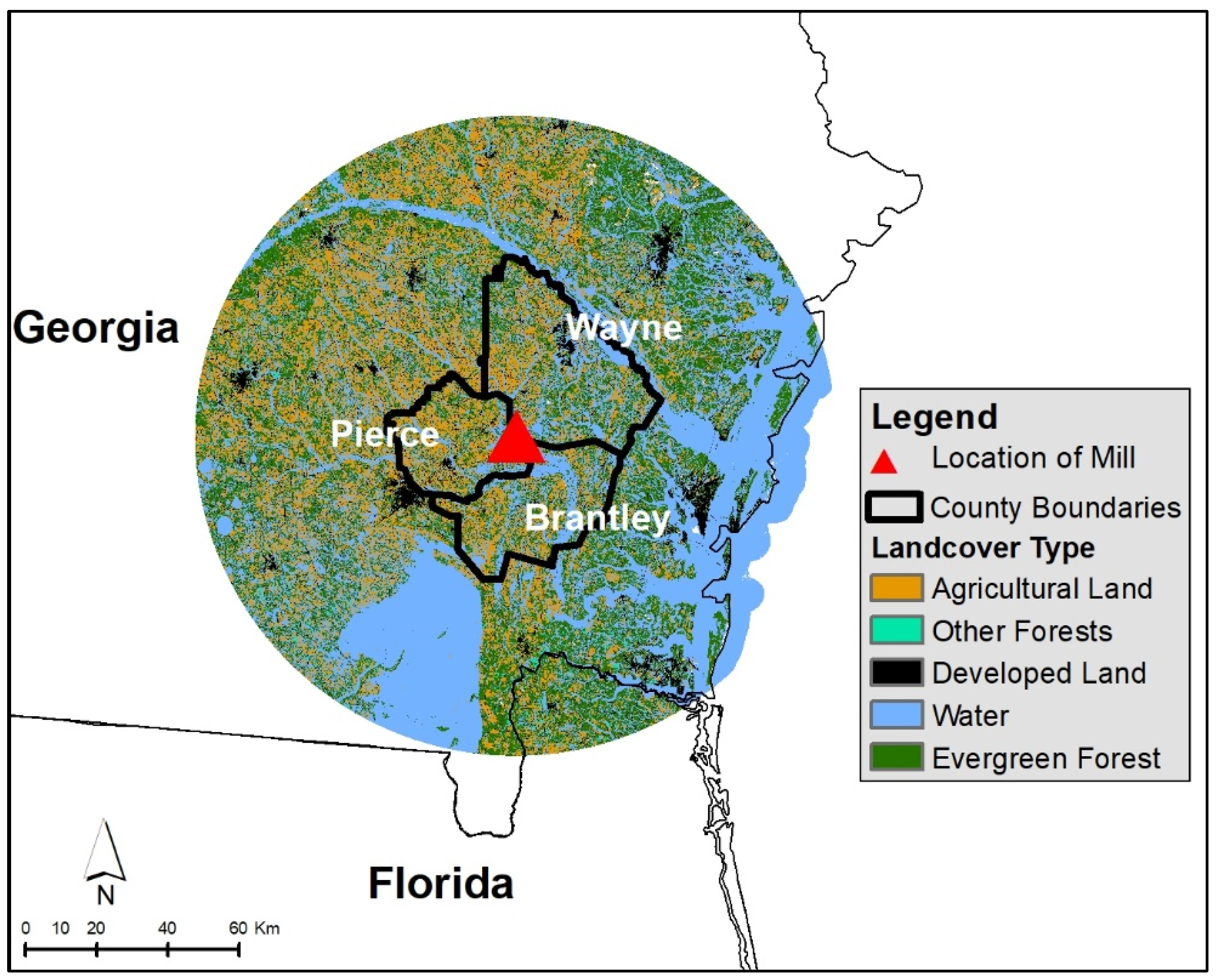
2.1. Study Area

The reference location of the pulp mill was at the intersection of Pierce, Wayne, and Brantley counties in South Georgia (Figure 1). The location was selected as South Georgia and North Florida have the largest concentration of pine plantations in the southern United States [4]. Additionally, the location of the pulp mill is well within the historical range of longleaf pine and ALRI’s significant geographic area where longleaf pine restoration is prioritized. We assumed that the pulpwood would be sourced within a radius of 90 km around the pulp mill, given the knowledge that wood procurement is restricted by the transportation cost [27,30]. We extracted evergreen land cover from the 2016 National Land Cover Database (NLCD) within the sourcing radius [31]. NLCD 2016 is the nationwide publicly available data on the land cover at 30 m resolution with 96% accuracy for evergreen land cover [32]. Loblolly pine occupied approximately three million hectares (21%) of the total plantations within the sourcing radius [4]. The landscape was divided into 0.4 hectare (1.0 acre) grids, where each grid had a certain percentage of the total area covered by evergreen land ranging between 0% and 100%. The percentage of evergreen land cover on each grid was based on the actual land cover data.

2.2. Forest Management Scenarios

We selected three scenarios for assessing the impact of the gradual adoption of longleaf pine at the landscape level on the wood procurement cost of the selected pulp mill (Table 1). In Scenario 1 (control), the pulpwood was sourced only from loblolly pine stands, and clearcut loblolly pine stands were not replaced by longleaf pine during the simulation period. In Scenario 2, the pulpwood was sourced from loblolly and longleaf pine stands, and 10% of the clearcut loblolly pine stands were randomly replaced by longleaf pine for each year present in the simulation period. Additionally, longleaf pine stands were managed using periodic burns. Pine straw was not collected in the years when the stand was burned. Scenario 3 resonates with Scenario 2, except that no periodic burns were undertaken on longleaf pine stands to rake pine straw. The income from pine straw significantly increases the profitability of landowners [9,10,11]. A 10% replacement rate was selected as it corresponds to ALRI’s goal of restoring longleaf pine across 3.2 million hectares, i.e., approximately 9% of the original longleaf pine area.
We included pine straw raking in our scenarios as the use of pine straw in landscaping has significantly grown over time. It is well known that pine straw maintains soil moisture, reduces weed growth, prevents soil compaction and erosion, protects plants from freezing conditions, and improves the soil structure over time [33,34]. Therefore, the demand for pine straw has gone up over time. For instance, the total revenue from pine straw in Georgia grew from USD 15.5 million in 1999 to USD 60–80 million between 2010 and 2017 [35]. Per Dickens et al. (2012) [36], the longleaf pine straw attracts higher prices (USD 0.65 to 1.20/bale) than loblolly pine (USD 0.25 to 0.40/bale). Pine straw suppliers and retailers usually prefer species with long needles such as longleaf pine that grow between 16 and 45 cm, compared to smaller loblolly pine needles that typically grow between 13 and 22 cm [37]. We acknowledge that pine straw raking on a loblolly pine stand is not common in the study area. Hence, income from pine straw raking was only included for longleaf pine. Pine straw prices (Table 2) were determined based on payments to the forest landowners [36].
In the southern United States, restoring the longleaf pine ecosystem requires converting existing loblolly pine stands to longleaf pine forests. To limit loblolly pine regeneration during the first few years, those sites require prescribed fire as a primary tool [41,42]. These few years are also attributed to longleaf pine’s unique “grass stage”, in which the terminal bud remains at the soil’s surface and growth is partitioned toward the root system rather than the stem. During this stage, seedlings become more resistant to low-intensity surface fires and less responsive to intensive silvicultural treatments, resulting in slower growth than the loblolly pines at the same age [5,6,12]. In the absence of prescribed fire, longleaf pine restoration sites were poised to become hardwood-dominated in the coming decades [43]. In addition, longleaf pine has lower Nitrogen and Phosphorous gain response than loblolly pine [37]. As a result, we have included burning as a possible option for longleaf pine management.

2.3. Economic Analysis

We used the growth and yield model developed by Gonzalez-Benecke et al. (2012) [44] and Gonzalez-Benecke et al. (2013) [45] for undertaking a stand-level economic analysis ascertaining the optimal rotation ages of a hectare of loblolly and longleaf pine stands. Three roundwood products were characterized based on stem diameter (outside bark) at breast height (dbh) and top diameter (td): sawtimber (dbh = 30.5 cm; td = 20.3 cm), and chip-n-saw (dbh = 20.3 cm, td = 15.2 cm), and pulpwood (dbh = 15.2 cm, td = 5.1 cm) for determining the optimal rotation ages.
The optimal rotation age was determined using the Faustmann Model (1849) [46], as shown in Equation (1):
〖LEV〗_t = (〖NPV〗_t × (〖1 + r)〗^t)/(〖(1 + r)〗^t − 1)
where Land Expectation Value (LEV in USD /ha) is the present value of profit at a given rotation age (t) over perpetuity, r is the real discount rate, t is the length of rotation in years, and NPV at a rotation age (t) is comprised of subtracting the present values of all the costs (establishment cost, fertilization, and annual taxes) from the present value of income from standing timber (Equation (1)). LEV represents a maximum amount to buy bare land at the beginning of a forest rotation, which helps to make a reasonable comparison between loblolly and longleaf pine. A real discount rate of 5% was used to reflect the range between 5 and 7%, commonly used for assessing forest investment in the southern United States [47]. We used a site index of 21.3 m for loblolly pine and 15.2 m for longleaf pine at the base age of 25 years to ensure equivalency across selected forest management scenarios between loblolly and longleaf pines. Details of management costs are reported in Table 2. The thinning age was determined based on the literature [12,48], i.e., when the total weight of the removed pulpwood reached at least 62 t/ha, the basal area reached 27–35 m2/ha, and Quadratic Mean Diameter was ≥15.5 cm. The thinning intensity was based on the residual basal area of 18.2 m2/ha [49] (Harrington 2001).

2.4. Model Assumptions

The total annual pulpwood capacity of the mill was assumed to be 450,000 metric tons. The age-class distribution data for loblolly pine (Figure 2) were extracted from EVALIDator [4] within the sourcing radius of the pulp mill. Grids were then randomly assigned an age class matching the age class distribution at the landscape level. The road distance from each grid to the pulp mill was calculated with the Origin-Destination cost matrix using the network analysis tool in ArcMAP [49]. The total pulpwood procurement cost for each grid was estimated by multiplying pulpwood quantity (t), the distance of the grid from the pulp mill (km), and unit transportation cost (USD/t/km). The pulpwood quantity available at a grid was a function of age class and total percent area under evergreen land cover. We used selected growth and yield models for ascertaining total pulpwood availability at a given stand age. Procurement purchases in the southern United States utilize a “minimum haul distance” structure, where any wood hauled within a minimum distance from the mill costs a fixed transportation cost, and then the cost increases incrementally. Therefore, the unit transportation cost was USD 0.07 t/km up to 60 km and USD 0.08 t/km for each additional km [30]. We avoided roads that did not allow gross weight beyond 37,000 t following regulatory constraints. The simulation model was based on the following assumptions: (a) there is no change in the stumpage price of pulpwood (received by landowners) over time, (b) there is no change in the forest management practices, and (c) the pulp mill sourced the same amount of pulpwood annually within the sourcing radius.

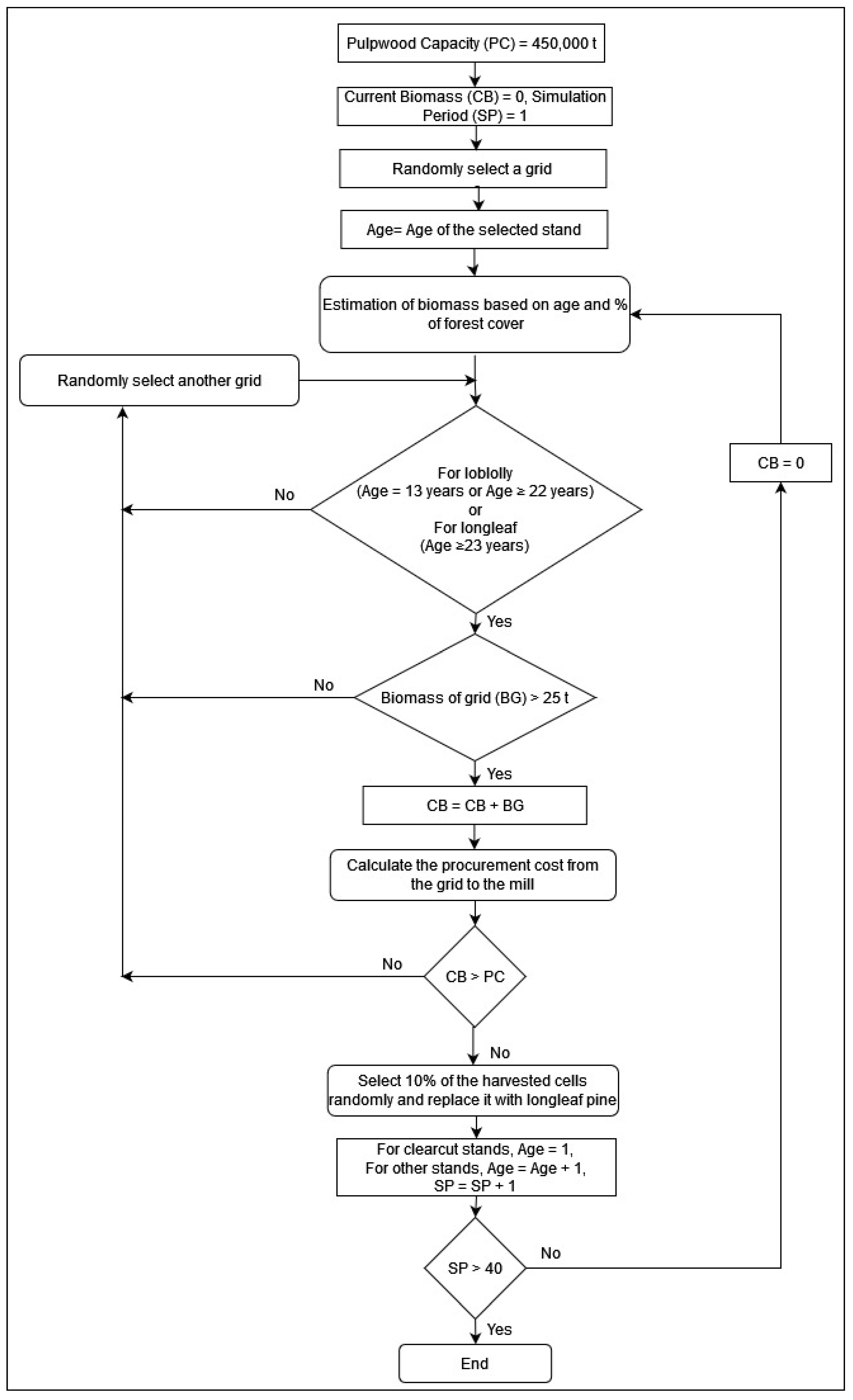
2.5. Simulation Model

We followed Dwivedi et al. (2012) [24] to develop a suitable simulation-based model based on the flowchart reported in Figure 3. As noticed, our model randomly harvests from eligible (based on current stand age and minimum pulpwood availability) grids at a given year rather than selecting grids based on their distance from the pulp mill. This change brings additional credibility to the developed model by mimicking the field realities to a larger extent. We developed our model in Python 3.8.1. We also suitably adopted the developed model to include the adoption of longleaf pine after the clearcut of loblolly pine at the selected rate over the simulation period. Total distance traveled, maximum distance traveled, total pulpwood available at the landscape after procurement, and changes in the age class distribution were recorded for each year of the simulation period.

2.6. Sensitivity Analysis

The profitability of growing longleaf or loblolly pine species is based on expected cash flows that are inherently uncertain. Uncertainties associated with timber procurement costs are due to weather, trucking logistics, competition, fuel cost volatility, and policy changes, as well as the development of new technologies [50,51]. Changes in the real discount rate significantly affect the LEV and the optimal rotation ages [52]. Therefore, we performed a sensitivity analysis by changing the real discount rate and transportation cost separately by ±40% from the base rates and costs used in the study for ascertaining the effects on the LEVs (Equation (1)).

2.7. Results

Pulpwood yields for loblolly and longleaf pines are reported in Figure 4. Loblolly pine is observed to have rapid growth, whereas longleaf pine has relatively slower growth. Longleaf pines are known for their unique grass and bottlebrush stage when vertical growth is slow, and the bulk of the growth is on root development [53]. Optimal rotation ages of longleaf and loblolly pines with their respective LEVs are reported in Table 3. The LEV of longleaf pine in Scenario 3 was higher than in Scenario 2 by USD 571/ha, with an optimal rotation age of 23 years. In contrast, the rotation age of longleaf pine in Scenario 2 was 29 years. The LEV of longleaf pine in Scenario 3 was lower than the LEV of loblolly pine by USD 280/ha.
To better explain any shifts in the overall pulpwood availability in the landscape (Figure 5), the original wood basket area was reduced to the maximum distance traveled during the simulation period for all scenarios. Pulpwood availability increased from the 7th to the 13th year of the simulation period for all the scenarios. This corresponds to the stand age in Figure 4, when the pulpwood yield of loblolly pine starts to increase. Pulpwood availability was highest for Scenario 1 until the 32nd year of the simulation period because of the higher pulpwood yield in the earlier years of loblolly pine and the slower growth of longleaf pine. As longleaf pine moved from the grass to the growth stage, pulpwood availability in the landscape (Scenarios 2 and 3) also increased. After the 32nd year of the simulation period, the highest pulpwood available was in Scenario 2. This difference was due to a positive linear relationship between the pulpwood yield and rotation age of longleaf pine in respective scenarios. The rotation age for longleaf pine in Scenario 2 was 29 years, with a yield of 146.8 t/ha, while it was 23 years with a yield of 97.3 t/ha for Scenario 3. The difference in rotation ages is due to periodic burn and pine straw raking across selected scenarios. A Welch two-sample t-test showed no statistically significant difference in pulpwood availability between Scenarios 2 and 3, but there were significant differences with Scenario 1.
The distribution of pulpwood sourced either from a thinned stand or a clearcut stand at a given year of the simulation period is shown in Figure 6. The pulpwood was sourced in a consistent manner across all the scenarios. Pulpwood was sourced from clearcut stands over the simulation period.
Figure 7 shows the trajectory of age class distribution at the landscape level over the simulation period. While the species composition differed, age class composition did not differ between scenarios. The areas covered by age classes 0–10 years and 11–20 years remained almost equivalent to the original age class distribution at the end of the simulation period. In comparison, the area under the age class > 40 years increased. Of the three scenarios, age class 31–40 years lost area (40%), and age class > 40 years gained area (200%) compared to the initial age class distribution. Figure 7 reflects upon the results reported in Figure 6, i.e., as most pulpwood was collected from clearcut and thinned stands, the least areas were occupied by age classes 21–30 years, followed by 11–20 years. Clearcut age for loblolly pine was 21 years, longleaf pine in Scenario 2 was 29 years, and longleaf pine in Scenario 3 was 23 years. The thinning age for loblolly pine was 13 years. Therefore, it is evident that the respective age classes during thinning and clearcut covered the least area in the landscape. An increase was expected in the area under the age class > 40 years, as some stands remained permanently in the landscape due to insufficient pulpwood demand. The maximum number of age classes observed at years 15, 30, and 40 of the simulation period were 56, 76, and 84, respectively. There was no difference in the number of age classes for all scenarios during the simulation periods. The number of age classes increased over the simulation period. As shown in Figure 7, the area of older-age stands increased with time. This remains true because some stands remain unharvested due to insufficient pulpwood per grid.
The total pulpwood sourced from loblolly and longleaf pines is reported in Figure 8. Only in the 24th year of the simulation period did the pulpwood start to procure longleaf pine for Scenario 3. The same was found in the 30th year of the simulation period for Scenario 2. This was anticipated because the longleaf pine plantations that replaced clearcut loblolly pine in the first year of the simulation period attained optimal rotation ages of 23 and 29 years for Scenario 2 and Scenario 3, respectively.
The distribution of the total distance covered to source the required pulpwood for all scenarios is shown in Figure 9. A minimal difference between scenarios was observed until the 23rd year of the simulation period. The least total distance was covered by Scenario 3 from the 24th year of the simulation period to the 40th year of the simulation period. This is reflected in Figure 8, where longleaf pine is being harvested along with loblolly pine in Scenario 3 from the 24th year of the simulation period. Similarly, we observe a lesser total distance covered in Scenario 2 than in Scenario 1 from the 30th year of the simulation period. When longleaf pine stands were harvested in Scenarios 2 and 3 (Figure 8), the total distance covered to procure pulpwood was smaller than in Scenario 1. Findings similar to the total distance traveled were observed with maximum distance traveled (Figure 10) and total cost of procurement (Figure 11). This was accompanied by a minimal difference in maximum distance covered between Scenarios 1 and 3 until the 30th year of the simulation period, resulting in the maximum total cost of procurement for Scenario 1 from the 30th year of the simulation period. Hence, when longleaf pine attained clearcut age in Scenarios 2 and 3, a lesser distance was traveled to procure a higher percentage of pulpwood, thereby reducing the total cost of procurement for the pulp mill compared to Scenario 1, where the pulp mill only procured loblolly pine.
A paired-sample t-test was conducted to test the difference in total cost, maximum distance traveled, and total distance traveled for wood procurement between Scenario 1 and both Scenarios 2 and 3. p-values of 0.79, 0.90, and 0.68 were observed between Scenario 1 and Scenario 2, and 0.028, 0.29, and 0.07 between Scenario 1 and Scenario 3 for total procurement cost, maximum distance traveled, and total distance traveled, respectively. Therefore, there was no significant difference between Scenario 1 and Scenarios 2 and 3 for maximum distance, total cost, and total distance over the simulation period.
We selected all the scenarios for undertaking sensitivity analyses. Among the other outputs generated through the simulated data, we only report the total cost of wood procurement (Table 4). The change in the total cost of wood procurement was directly proportional to the change in transportation cost, while it was indirectly proportional to the real discount rate. The percentage changes from the base values were greater for a given change in the transportation cost than with a change in the real discount rate. Therefore, the total cost of wood procurement was more sensitive to a change in transportation cost than to a change in the real discount rate.

3. Discussion

The profitability of wood-consuming mills is affected by transportation costs, which cover approximately 25% of the procurement costs [47]. Several initiatives are promoting longleaf pine restoration in the southern United States when the current area of loblolly pine has remained unchanged. Hence, this study assesses the change in the procurement cost when 10% of clearcut loblolly pine is replaced each year by longleaf pine at the landscape level over a 40-year simulation period for analyzing the impact of longleaf pine restoration on the wood procurement cost.
Pulpwood availability was highest for Scenario 1 until the 32nd year of the simulation period due to the higher pulpwood yield in the earlier years of loblolly pine and the slower growth of longleaf pine. As longleaf pine moved from the grass to the growth stage, the pulpwood available in the landscape (Scenarios 2 and 3) also increased. After the 32nd year of the simulation period, Scenario 2 had the highest amount of pulpwood availability. Prescribed fire has been shown to increase the yield of longleaf pine [40]. We found no significant difference in the pulpwood yield of longleaf pine in Scenarios 2 and 3 (Figure 4) based on the models developed by Gonzalez-Benecke et al. (2013) [45] and Gonzalez-Benecke et al. (2012) [44]. However, we found a significant difference in total pulpwood availability at the landscape level between Scenarios 2 and 3 (Figure 5). This is due to the difference in rotation age (year 29 for Scenario 2 and year 23 for Scenario 3) primarily due to pine straw collection for longleaf pine. Scenario 2 involves burning longleaf pine stands, resulting in a loss of revenue from pine straw for landowners. The longer rotation age in Scenario 2 indicates an additional six years of longleaf pine volume in the landscape, but in Scenario 3 those stands are already clearcut, resulting in a significant difference in pulpwood availability.
Results reveal that the age structure of surrounding forest plantations changes in time and space. The total number of plantation age classes present in the landscape increases with an increase in the simulation period. Mature age classes remained in the landscape, covering a larger area than the original area covered, which contradicts the result presented by Dwivedi et al. (2012) [24], where mature age classes are lost permanently with an increase in mill capacity. Old-growth forests are linked with species richness and better habitat quality [54]. Therefore, an increase in the area of mature age classes, retaining original age class distribution, helps to maintain landscape-level variability and causes an even distribution of age class in the landscape, thus maintaining the local biodiversity and ecological stability that longleaf and loblolly pine support.
The procurement process attained stability that we usually observe in a managed landscape, where most pulpwood was procured from clearcut stands than from thinned stands (Figure 6). The total distance traveled, maximum distance traveled, and total cost of procurement show a similar pattern across scenarios (Figure 9, Figure 10 and Figure 11). Differences between selected scenarios were observed after the clearcut age of longleaf pine in respective scenarios for total distance traveled, maximum distance traveled, and total cost of procurement. Scenario 1 differed from Scenario 2 from the 24th year of the simulation period and from Scenario 3 from the 30th year of the simulation period. When longleaf pine attained clearcut age in Scenarios 2 and 3, less distance was traveled to procure pulpwood, reducing the total cost of procurement for the pulp mill compared to Scenario 1, where the pulp mill only procured loblolly pine.
We utilized the NLCD database for our study, whose accuracy was 96% for evergreen landcover type compared to the current evergreen landcover. Hence, temporal and spatial mismatches can contribute to the uncertainty in the model’s outputs. We considered landscapes with only pine straw markets in our study; however, markets for pine straw are geographically limited and not available to landowners throughout the longleaf pine range. Future research can assess the role of pine straw income on the rotation ages, and thereby any impact on the total wood procurement cost. Additionally, our results show that older plantations remain in the landscape. Still, if there is an increase in the competition for pulpwood, there is limited evidence to understand how these plantations would be affected. Moreover, the simulation model does not consider landowners committed to managing loblolly pine or longleaf pine for products other than pulpwood. Studies have shown that sawmills are willing to pay a premium price for high-quality sawtimber, and longleaf pine is valued for high-quality poles and sawtimber [55,56]. Therefore, our model deviates somewhat from reality, where pulpwood is considered the only wood product in the selected landscape. Hence, spatial constraints to spread procurement in space, product, and time should be considered in future models for generating much more fine-scale information.
Furthermore, the study does not include risk, such as pest attacks and hurricanes, which can significantly impact the supply chain. Finally, the impact of modeled changes on the local biodiversity was not assessed. Spatial prioritization studies have shown that a higher probability exists for new longleaf pine plantations on those croplands and pasturelands that are closer to existing plantations supported by various federal and state programs [57]. We have included any potential land cover changes in the context of longleaf plantations in this study. However, this could be another avenue for future research to better estimate any changes in wood procurement costs considering direct and indirect land use changes in the vicinity of a wood-consuming mill.

4. Conclusions

Several initiatives are currently promoting longleaf pine restoration in the southern United States. Hence, our study simulates spatiotemporal changes in the age distribution and wood procurement costs when 10% of clearcut loblolly pine stands each year are replaced by longleaf pine at the landscape level. It was assumed that the pulp mill would only procure pulpwood from the surrounding stands over a 40-yers simulation period. A simulation-based approach was used to estimate any changes in the wood procurement cost of the pulp mill located in the center of the landscape.
Based on simulation results, we found that the total pulpwood availability, total distance traveled, maximum distance traveled, and total cost of procurement show a similar pattern across scenarios. Total pulpwood, total distance, maximum distance, and total cost of procurement declined when most of the pulpwood was procured from clearcut stands. The values of the same variables increased when most pulpwood was procured from the thinned stands. Throughout the simulation period, the procurement process attained the stability that we usually observe, where most of the pulpwood was procured from clearcut stands than from thinned stands across scenarios. Differences between scenarios were observed after the clearcut age of longleaf pine in respective scenarios for total distance traveled, maximum distance traveled, and total cost of procurement. Scenario 1 differed from Scenario 2 from the 24th year of the simulation period and with Scenario 3 from the 30th year of the simulation period.
Our results show that there is no significant statistical difference in total pulpwood availability, total distance traveled, maximum distance traveled, and total cost of wood procurement over a 40-year simulation period across scenarios. Therefore, replacing 10% of clearcut loblolly pine with longleaf pine does not significantly change the procurement cost for mills but does change the age class structure of the landscape. With an anticipated increase in the area of longleaf pine plantations, understanding there is no difference in procurement cost is beneficial for landowners and particularly for pulp mill operators that are concerned about the additional cost of procuring longleaf pine.
We also found that mature plantations covered a larger area than the original age class distribution, in addition to significantly less alteration in the original age class structure throughout the landscape over the simulation period. Comparable results for age class distribution were observed by Dwivedi et al. (2012) [24], with only one species at the landscape level. Thus, the establishment of a pulp mill that procures longleaf pine along with loblolly pine helps to maintain the uneven age class distribution in the landscape, potentially supporting species richness and ecological stability.
We recommend increasing awareness among forest landowners and mill operators regarding the procurement cost of longleaf pine in comparison to loblolly pine through our study. We hope that the findings of this study will feed into ongoing deliberations regarding longleaf pine restoration across the southern United States. We hope that future research will further extend the model developed in this study to enhance our understanding of the role of longleaf pine restoration on the wood procurement cost for the wood-consuming mills located in South Georgia and other relevant geographies across the southern United States.

Author Contributions

K.P. collected the data, developed the model, and wrote the first draft of the manuscript. P.D. obtained the grant, conceptualized the research, edited the manuscript, and supervised the overall research. All authors have read and agreed to the published version of the manuscript.

Funding

This work is supported by the United States Department of Agriculture National Institute Food and Agriculture through an award # 2017-67023-26274.

Institutional Review Board Statement

Not applicable.

Informed Consent Statement

Not applicable.

Data Availability Statement

Growth and yield model developed by Gonzalez-Benecke et al. (2012) [44] and Gonzalez-Benecke et al. (2013) [45] can be accessed at Carbon Resources Science Center (https://carboncenter.ifas.ufl.edu, accessed on 4 July 2022). FIA database can be accessed at https://www.fia.fs.fed.us, accessed on 4 July 2022.

Conflicts of Interest

The authors declare no conflict of interest.

References

  1. Brandeis, T.J. Forests of Georgia, 2013. In Resource Update FS-38; US Department of Agriculture Forest Service Southern Research Station 4: Asheville, NC, USA, 2015; Volume 38, pp. 1–4. [Google Scholar]
  2. Stanturf, J.; Kellison, R.C.; Broerman, F.S.; Jones, S.B. Productivity of southern pine plantations: Where are we and how did we get here? J. For. 2003, 101, 26–31. [Google Scholar]
  3. Oswalt, M.C.; Cooper, J.A.; Brockway, D.G.; Brooks, H.W.; Walker, J.L.; Connor, K.F.; Oswalt, S.N.; Conner, R.C. History and current condition of longleaf pine in the southern United States. In General Technical Report-Southern Research Station, USDA Forest Service SRS-166; Southern Research Station: Asheville, NC, USA, 2012. [Google Scholar]
  4. Miles, P.D. Forest Inventory EVALIDator Web-Application Version 1.6. 0.03; US Department of Agriculture, Forest Service, Northern Research Station: St. Paul, MN, USA, 2019. Available online: https://apps.fs.usda.gov/fiadb-api/evalidator (accessed on 8 May 2019).
  5. Van Lear, H.D.; Carroll, W.D.; Kapeluck, P.R.; Johnson, R. History and restoration of the longleaf pine-grassland ecosystem: Implications for species at risk. For. Ecol. Manag. 2005, 211, 150–165. [Google Scholar] [CrossRef]
  6. Gilliam, F.S.; Platt, W.J. Conservation and restoration of the Pinus palustris ecosystem. Appl. Veg. Sci. 2006, 9, 7–10. [Google Scholar] [CrossRef] [Green Version]
  7. Outcalt, W.K.; Brockway, D.G. Structure and composition changes following restoration treatments of longleaf pine forests on the Gulf Coastal Plain of Alabama. For. Ecol. Manag. 2010, 259, 1615–1623. [Google Scholar] [CrossRef]
  8. Johnsen, H.K.; Butnor, J.R.; Kush, J.S.; Schmidtling, R.C.; Nelson, C.D. Hurricane Katrina winds damaged longleaf pine less than loblolly pine. South. J. Appl. For. 2009, 33, 178–181. [Google Scholar] [CrossRef] [Green Version]
  9. Susaeta, A.; Gong, P. Economic viability of longleaf pine management in the Southeastern United States. For. Policy Econ. 2009, 100, 14–23. [Google Scholar] [CrossRef]
  10. Upadhaya, S.; Dwivedi, P. The role and potential of blueberry in increasing deforestation in southern Georgia, United States. Agric. Syst. 2019, 173, 39–48. [Google Scholar] [CrossRef]
  11. Paudel, K.; Dwivedi, P. Economics of Southern Pines with and without Payments for Environmental Amenities in the US South. Front. For. Glob. Chang. 2021, 4, 35. [Google Scholar] [CrossRef]
  12. Hatchell, G.E.; Marx, D.H. Response of longleaf, sand, and loblolly pines to Pisolithus ectomycorrhizae and fertilizer on a sandhills site in South Carolina. For. Sci. 1987, 33, 301–315. [Google Scholar]
  13. Wahlgren, H.E.; Schumann, D.R.; Bendtsen, B.A.; Ethington, R.L.; Galligan, W.L. Properties of Major Southern Pines: Part I: Wood Density Survey. Part II: Structural Properties and Specific Gravity; Forest Products Lab: Madison, WI, USA, 1975. [Google Scholar]
  14. Landers, J.L.; Van Lear, D.H.; Boyer, W.D. The longleaf pine forests of the southeast: Requiem or renaissance? J. For. 1995, 93, 39–44. [Google Scholar]
  15. Palmgren, M.; Rönnqvist, M.; Rebrand, P. A solution approach for log truck scheduling based on composite pricing and branch and bound. Int. Trans. Oper. Res. 2003, 10, 433–447. [Google Scholar] [CrossRef]
  16. Abbas, D.; Handler, R.; Dykstra, D.; Hartsough, B.; Lautala, P. Cost analysis of forest biomass supply chain logistics. J. For. 2013, 111, 271–281. [Google Scholar] [CrossRef]
  17. Haridass, K.; Valenzuela, J.; Yucekaya, A.D.; McDonald, T. Scheduling a log transport system using simulated annealing. Inf. Sci. 2014, 264, 302–316. [Google Scholar] [CrossRef]
  18. Coelho, C.L.; Gagliardi, J.; Renaud, J.; Ruiz, A. Solving the vehicle routing problem with lunch break arising in the furniture delivery industry. J. Oper. Res. Soc. 2016, 67, 743–751. [Google Scholar] [CrossRef]
  19. Conrad, J.L., IV; Greene, W.D.; Hiesl, P. The evolution of logging businesses in Georgia 1987–2017 and South Carolina 2012–2017. For. Sci. 2018, 64, 671–681. [Google Scholar] [CrossRef]
  20. Möller, B.; Nielsen, P.S. Analysing transport costs of Danish forest wood chip resources by means of continuous cost surfaces. Biomass Bioenergy 2007, 31, 291–298. [Google Scholar] [CrossRef]
  21. Ince, J.P.; Kramp, A.D.; Skog, K.E.; Yoo, D.I.; Sample, V.A. Modeling future US forest sector market and trade impacts of expansion in wood energy consumption. J. For. Econ. 2011, 17, 142–156. [Google Scholar]
  22. Polyakov, M.; Teeter, L.D.; Jackson, J.D. Econometric analysis of Alabama’s pulpwood market. For. Prod. J. 2005, 55, 41–44. [Google Scholar]
  23. Aksoy, B.; Cullinan, H.; Webster, D.; Gue, K.; Sukumaran, S.; Eden, M.; Sammons, N. Woody biomass and mill waste utilization opportunities in Alabama: Transportation cost minimization, optimum facility location, economic feasibility, and impact. Environ. Prog. Sustain. Energy 2011, 30, 720–732. [Google Scholar] [CrossRef]
  24. Dwivedi, P.; Bailis, R.; Carter, D.R.; Sharma, A. A landscape based approach for assessing spatiotemporal impacts of forest biomass-based electricity generation on the age structure of surrounding forest plantations in the Southern United States. GCB Bioenergy 2012, 4, 342–357. [Google Scholar] [CrossRef]
  25. Sun, C.; Zhang, D. Timber harvesting margins in the Southern United States: A temporal and spatial analysis. For. Sci. 2006, 52, 273–280. [Google Scholar]
  26. Mogus, A.; Stennes, B.; van Kooten, G.C. Canada–US softwood lumber trade revisited: Substitution bias in the context of a spatial price equilibrium framework. For. Sci. 2006, 52, 411–421. [Google Scholar]
  27. Anderson, M.N.; Germain, R.H.; Bevilacqua, E. Geographic information system-based spatial analysis of sawmill wood procurement. J. For. 2011, 109, 34–42. [Google Scholar]
  28. Susaeta, A.; Gong, P.; Adams, D. Implications of the reservation price strategy on the optimal harvest decision and production of nontimber goods in an even-aged forest stand. Can. J. For. Res. 2020, 50, 287–296. [Google Scholar] [CrossRef]
  29. Forman, R.T.; Godron, M. Patches and structural components for a landscape ecology. BioScience 1981, 31, 733–740. [Google Scholar]
  30. TMS. TimberMart-South: Southwide Average Prices. Athens, GA. Available online: http://www.timbermart-south.com (accessed on 17 April 2019).
  31. USDA Natural Resources Conservation Service. NRCS Regional Conservation Partnership Program—Longleaf Pine Range. USDA Natural Resources Conservation Service. 2018. Available online: https://data.nal.usda.gov/dataset/nrcs-regional-conservation-partnership-program-longleaf-pine-range (accessed on 25 May 2019).
  32. Homer, C.; Dewitz, J.; Jin, S.; Xian, G.; Costello, C.; Danielson, P.; Gass, L.; Funk, M.; Wickham, J.; Stehman, S.; et al. Conterminous United States land cover change patterns 2001–2016 from the 2016 National Land Cover Database. ISPRS J. Photogramm. Remote Sens. 2020, 162, 184–199. [Google Scholar] [CrossRef]
  33. Chalker-Scott, L. Impact of mulches on landscape plants and the environment—A review. J. Environ. Hortic. 2007, 25, 239–249. [Google Scholar] [CrossRef]
  34. Makus, D.J.; Tiwari, S.C.; Pearson, H.A.; Haywood, J.D.; Tiarks, A.E. Okra production with pine straw mulch. Agrofor. Syst. 1994, 27, 121–127. [Google Scholar] [CrossRef]
  35. Dickens, E.D.; Morris, L.; Clabo, D.; Ogden, L. Pine straw raking and growth of southern pine: Review and recommendations. Forests 2020, 11, 799. [Google Scholar] [CrossRef]
  36. Dickens, E.D.; David, M.J.; Bargeron, C.T.; Morris, L.A.; Ogden, L.A.; McElvany, B.C. A Summary of pine straw yields and economic benefits in loblolly, longleaf and slash pine stands. Agrofor. Syst. 2012, 86, 315–321. [Google Scholar] [CrossRef]
  37. Dickens, E.D.; John, S.; Moorhead, D.J. Economics of Growing Loblolly, Longleaf, and Slash Pine to Various Rotation Ages with Three Stumpage Price Sets, Four Establishment Cost Sets, Four Discount Rates, with and without Pine Straw—Soil Expectation Value; University of Georgia Warnell School of Forestry and Natural Resources: Athens, GA, USA, 2014. [Google Scholar]
  38. Maggard, A.; Barlow, B. Costs & trends of southern forestry practices, 2016. In Publication FOR-2051, Alabama Cooperative Extension System; Auburn University: Auburn, AL, USA, 2018. [Google Scholar]
  39. Gonzalez-Benecke, A.C.; Samuelson, L.J.; Martin, T.A.; Cropper, W.P., Jr.; Johnsen, K.H.; Stokes, T.A.; Butnor, J.R.; Anderson, P.H. Modeling the effects of forest management on in-situ and ex-situ longleaf pine forest carbon stocks. For. Ecol. Manag. 2015, 355, 24–36. [Google Scholar] [CrossRef] [Green Version]
  40. Haywood, J.D. Influence of herbicides and felling, fertilization, and prescribed fire on longleaf pine growth and understory vegetation through ten growing seasons and the outcome of an ensuing wildfire. New For. 2011, 41, 55–73. [Google Scholar] [CrossRef]
  41. Binkley, D. Ten-year decomposition in a loblolly pine forest. Can. J. For. Res. 2002, 32, 2231–2235. [Google Scholar] [CrossRef]
  42. Knapp, B.O.; Wang, G.G.; Hu, H.; Walker, J.L.; Tennant, C. Restoring longleaf pine (Pinus palustris Mill.) in loblolly pine (Pinus taeda L.) stands: Effects of restoration treatments on natural loblolly pine regeneration. For. Ecol. Manag. 2011, 262, 1157–1167. [Google Scholar] [CrossRef]
  43. Matusick, G.; Hudson, S.J.; Garrett, C.Z.; Samuelson, L.J.; Kent, J.D.; Addington, R.N.; Parker, J.M. Frequently burned loblolly–shortleaf pine forest in the southeastern United States lacks the stability of longleaf pine forest. Ecosphere 2020, 11, e03055. [Google Scholar] [CrossRef]
  44. Gonzalez-Benecke, A.C.; Jokela, E.J.; Martin, T.A. Modeling the effects of stand development, site quality, and silviculture on leaf area index, litterfall, and forest floor accumulations in loblolly and slash pine plantations. For. Sci. 2012, 58, 457–471. [Google Scholar] [CrossRef]
  45. Gonzalez-Benecke, A.C.; Gezan, S.A.; Martin, T.A.; Cropper, W.P., Jr.; Samuelson, L.J.; Leduc, D.J. Individual tree diameter, height, and volume functions for longleaf pine. For. Sci. 2013, 60, 43–56. [Google Scholar] [CrossRef] [Green Version]
  46. Faustmann, M. On the Determination of the Value which Forest Land and Immature Stands Possess for Forestry; Gane, M., Translator; Oxford Institute: Oxford, UK, 1849; Paper 42; p. 1968. [Google Scholar]
  47. Conrad, J.L., IV. Costs and challenges of log truck transportation in Georgia, USA. Forests 2018, 9, 650. [Google Scholar] [CrossRef] [Green Version]
  48. Harrington, T.B. Silvicultural Approaches for Thinning Southern Pines: Method, Intensity, and Timing; Georgia Forestry Commission: Macon, GA, USA, 2001. [Google Scholar]
  49. ESRI. ArcMap 10.8. 2020. Available online: https//desktop.arcgis.com (accessed on 4 July 2022).
  50. Wear, D.N.; Carter, D.R.; Prestemon, J. The US South’s Timber Sector in 2005: A Prospective Analysis of Recent Change. Gen. Tech. Rep. SRS-99; US Department of Agriculture, Forest Service, Southern Research Station: Asheville, NC, USA, 2007; Volume 29, p. 99. [Google Scholar]
  51. Keramati, A.; Lu, P.; Sobhani, A.; Haji Esmaeili, S.A. Impact of Forest Road Maintenance Policies on Log Transportation Cost, Routing, and Carbon-Emission Trade-Offs: Oregon Case Study. J. Transp. Eng. Part A Syst. 2020, 146, 04020028. [Google Scholar] [CrossRef]
  52. Harris, A.B.; Singleton, C.N.; Straka, T.J. Land Value Differentials Resulting from Variability between the Sales Comparison and Income Approaches in Timberland Valuation. Apprais. J. 2018, 86, 192–205. [Google Scholar]
  53. Patterson, W.T.; Knapp, P.A. Observations on a rare old-growth montane longleaf pine forest in central North Carolina, USA. Nat. Areas J. 2016, 36, 153–161. [Google Scholar] [CrossRef]
  54. Spies, T.A. Ecological concepts and diversity of old-growth forests. J. For. 2004, 102, 14–20. [Google Scholar]
  55. Schroeder, J.G.; Taras, M.A.; Clark, A. Stem and Primary Product Weights for Longleaf Pine Sawtimber Trees; Forest Service, US Department of Agriculture, Southeastern Forest Experiment Station: Asheville, NC, USA, 1975; Volume 139. [Google Scholar]
  56. Regmi, A.; Grebner, D.L.; Willis, J.L.; Grala, R.K. Sawmill Willingness to Pay Price Premiums for Higher Quality Pine Sawtimber in the Southeastern United States. Forests 2022, 13, 662. [Google Scholar] [CrossRef]
  57. Paudel, K.; Dwivedi, P.; Dickens, D. Factors affecting the spatial density of longleaf pine plantations under the Conservation Reserve Program in Georgia, United States. Trees For. People 2021, 3, 100045. [Google Scholar] [CrossRef]
Figure 1. Location of the pulp mill, selected initial sourcing radius (90 km), and the spatial distribution of evergreen forestlands [31].
Forests 13 01112 g001
Figure 2. Distribution of age classes for loblolly pine at the start of the simulation period in the study area.
Forests 13 01112 g002
Figure 3. The flowchart for simulating Scenario 3. Suitable changes are made for simulating other selected scenarios.
Forests 13 01112 g003
Figure 4. Distribution of pulpwood volume by stand age for loblolly and longleaf pine stands.
Forests 13 01112 g004
Figure 5. Distribution of total pulpwood availability at the landscape level over the simulation period. Scenarios 1, 2 and 3 are differentiated in Table 1.
Forests 13 01112 g005
Figure 6. Distribution of total pulpwood sourced from thinned and clearcut stands over the simulation period. Scenarios 1, 2 and 3 are differentiated in Table 1.
Forests 13 01112 g006
Figure 7. Distribution of area occupied by each age class within the sourcing radius (90 km) of the pulp mill during different years of the simulation period. Scenarios 1, 2 and 3 are differentiated in Table 1.
Forests 13 01112 g007
Figure 8. Distribution of pulpwood procured from each species over the simulation period. Results are reported only for Scenario 2 and Scenario 3, as longleaf pine is not present in the landscape in Scenario 1. Scenarios 2 and 3 are differentiated in Table 1.
Forests 13 01112 g008
Figure 9. Distribution of total distance traveled for sourcing pulpwood over the simulation period. Scenarios 1, 2 and 3 are differentiated in Table 1.
Forests 13 01112 g009
Figure 10. Distribution of maximum distance traveled over the simulation period. Scenarios 1, 2 and 3 are differentiated in Table 1.
Forests 13 01112 g010
Figure 11. Distribution of total cost of pulpwood procurement at different years of the simulation period. Scenarios 1, 2 and 3 are differentiated in Table 1.
Forests 13 01112 g011
Table 1. Scenarios selected for the study.
Scenario #Replacement by LongleafReplacementPine StrawPeriodic Burn
S1No0%NoNo
S2Yes10%YesYes
S3Yes10%YesNo
Table 2. Selected incomes (USD), costs (USD), and silvicultural treatments for estimating the optimal rotation age of a hectare of loblolly and longleaf pines in South Georgia, United States. The prices of timber products and silvicultural management costs were obtained from TMS (2019) [30] and Maggard and Barlow (2018) [38], respectively. Fertilization volume and applications are as per the productivity of sandy soils in the Lower Coastal Plain [36]. Longleaf pine stands that are suitable for raking pine straw are commonly raked starting canopy closure until the first thinning [36]. Hence, pine straw raking started from year eight until the first thinning age for longleaf pine. We used Gonzalez-Benecke et al. (2015) [39] to estimate annual needle fall and pine straw yields. We did not rake pine straw for the years when the longleaf pine stand was burned [40].
Treatment/Income SourceYearAmount
Pulpwood Price USD 9.9/t
Sawtimber Price USD 21.4/t
Chip-n-Saw Price USD 15.7/t
Cost Sources
Mechanical site preparationYear 0USD 255.5/ha
Planting Year 1USD 214.4/ha
Management CostAll yearsUSD 12.3/ha/year
TaxAll yearsUSD 12.35/ha/year
Loblolly Pine
Chemical site preparationYear 0USD 191.9/ha
Seedlings USD 149.5/ha
Herbaceous weed controlYear 1USD 141.1/ha
ThinningYear 13USD 9.9/t
Thinning intensity 45%
Fertilize (140 DAP + 252 Urea)Years 2 and 13USD 0.4/kg
Longleaf Pine (Scenario 2)
Site prep burnYear 0USD 61.7/ha
Seedlings USD 370/ha
Weed controlYear 1USD 141.1/ha
First prescribed burnYear 9USD 34.5/ha
Burning frequencyEvery three years, between 9th and 23rd yearsUSD 34.5/ha
Pine straw price Year 8–Year 23 (no pine straw collection in the years when the site was burned)USD 142/t
Longleaf Pine (Scenario 3)
Site prep burnYear 0USD 61.7/ha
Seedlings USD 375.6/ha
Weed controlYear 1USD 141/ha
First prescribed burnYear 9USD 34.54/ha
Pine straw priceYears 8–Year 23USD 142 /t
Table 3. Land expectation value (LEV), optimal rotation age (years), pulpwood yield at the optimal rotation age, thinning age, and pulpwood yield at thinning age for loblolly and longleaf pines.
SpeciesLEV (USD /ha)Rotation AgePulpwood Yields at Rotation Age (t/ha)Thinning Age (years)Pulpwood Yield at Thinning Age (t/ha)
Loblolly Pine (S1, S2 and S3)307922531369
Longleaf Pine (S2)222829147-
Longleaf Pine (S3)27992397-
Table 4. Sensitivity analysis of the total cost of wood procurement (million USD) by changing the transportation cost and real discount rate by ±40%. Values reported are the average of 40-years of the simulation period. Values reported in parentheses are percentage changes from the base values. A higher discount rate has an inverse relation with NPV. With a decrease in NPV, rotation age also decreases, causing a decrease in the transportation cost.
Change (%)
FactorsScenarios+400−40
Change in Transportation CostS1402.4 (39.6)288.2172.2 (−40.1)
S2400.6 (39.3)287.5170.6 (−40.6)
S3397.0 (40.4)282.9169.0 (−40.0)
Change in Real Discount RateS1279.5 (−3.3)288.2293.6 (2.4)
S2278.8 (−3.3)287.5296.1 (3.2)
S3277.2 (−2.0)282.9285.7 (1.6)
Publisher’s Note: MDPI stays neutral with regard to jurisdictional claims in published maps and institutional affiliations.

