A Numerical Study of the Effect of Vegetative Windbreak on Wind Erosion over Complex Terrain

Abstract

Wind erosion is a typical issue for stone carvings in northwest China caves, and windbreaks such as shelterbelts have proven to be effective in mitigating wind erosion. This study has the main purpose of examining the effect of shelterbelts on alleviating the wind erosion degree of stone carvings. The applicability of the canopy model for reproducing the aerodynamic effects based on the realizable k–ε and LES model was examined by using a validation metric. The shelterbelt structure has been discussed with the goal of finding the optimum canopy structure to provide a guideline for designing shelterbelts. Compared with the LES model, the realizable k–ε model was adopted in this study based on its comprehensive performance. The results show that a canopy with porosity of φ = 30% and a width of 0.3 to 0.5 H has better sheltering efficiency. Compared to the case with no shelterbelt, the wind speed amplification coefficient decreased by 43%, and the significant decrease in the value of the wind speed amplification coefficient in the primary-harm wind direction demonstrates the effectiveness of the shelterbelt. By exploring preventive protection technology in the context of historical stone carving, this study can promote the practice of scientific and technological protection of cultural relics.

1. Introduction

Windbreaks such as shelterbelts and fences have been used around the world for centuries to protect soils from wind erosion [1,2,3,4,5,6,7]. A shelterbelt, as a kind of natural windbreak, creates resistance to the approaching airflow and forces the wind to reduce its speed. It has proven to be effective in mitigating wind erosion. The interaction between the shelterbelt and the airflow is complicated by the turbulent characteristics of the airflow and the complex structure of the shelterbelt [8]. Therefore, the prediction of the flow fields around the shelterbelt has been conducted by numerous researchers in recent decades [9,10,11,12,13,14].

There is a requirement for wind energy resource assessment [15] and pollutants dispersion [16], where the local wind fields are significantly affected by surrounding vegetation near mountain areas. Studies of simulated flow around shelterbelts over complex terrain have generated increasing interest in recent years [17,18,19,20]. Although researchers have made great progress in the studies of flow fields around shelterbelts over flat or simple terrains, there are few studies on flow fields over real complex terrain around shelterbelts. In addition, very limited studies have recently accounted for the relationship between the local flow characteristics and wind erosion of stone carvings and how to adjust the wind environment in the Grottoes by setting up a shelterbelt.

The shelter efficiency of shelterbelts is intrinsically related to the flow characteristics of the airflow around them, and the flow fields around the shelterbelt can be divided into the following major regions (Figure 1) [21]. The flow on the upstream of the shelterbelt (Region A) is known as the approach flow. Downstream of Region A, the flow is divided into two parts. The part that passes through the shelterbelt is called the bleed flow (Region C). The flow displaced over the shelterbelt is called the displaced flow (Region B). There is a quiet zone (region D) with a small area downwind of the bleed flow, followed by a mixed zone (region E) with a large area. Further downwind, the displaced flow is attached to the ground, which produces flow characteristics similar to those in Region A, and this zone is called the re-equilibration zone (Region F).

Numerous experiments have been conducted to measure flow around three-dimensional vegetation in a full-scale field [1,22,23,24]. The advantage of this method is that the full complexity of the flow characteristics is considered under real atmospheric conditions. However, this method is limited by low spatial resolution, and it is difficult to understand the shelterbelt aerodynamics mechanism. Wind tunnel experiments can control the inflow conditions, and the stationary flow conditions can be maintained throughout the entire experiment process [25,26,27,28]. However, they are also limited by spatial measurement points and require adherence to similarity criteria. With the rapid improvement of computer power and the development of computing software programs, the CFD technique has been widely used to investigate flow fields around shelterbelts [29,30,31]. CFD has some advantages compared to previous methods since it obtains flow characteristics of each position in the flow fields, and there are no problems with violating similarity requirements because simulations can be performed at full scale [32,33]. However, the accuracy and reliability of numerical simulation largely depend on the use of closure schemes and the setting of the operation of the software. For these reasons, field measurements are also imperative to verify the accuracy of CFD numerical simulations.

Until now, there have been two types of approaches to modeling vegetation’s effects on flow fields. One is to simulate vegetation with corresponding roughness, affecting the wind profile above the ground surface [34], and the other is to introduce a porous medium to represent a vegetation canopy model, creating resistance as the airflow passes through by including source terms for turbulent transportation equations and a drag term in the momentum equations [11,29,35,36]. The first approach is widely used in numerical studies on the flow fields around vegetation because of its convenience. However, the main problem with this method is that it can only roughly generate the general characteristics of airflow over the vegetation, and it can only provide the average velocity profile, which is insufficient for information regarding the turbulence characterization. The second approach is to use the canopy model, which is attracting increasing attention because of its ability to physically consider the drag effect from the vegetation.

In past simulation studies on the performance of windbreak, much research on canopy models with Reynolds Averaged Navier–Stokes (RANS) model has been carried out. They concluded that the performance of the RNG (Renormalization Group) and realizable k-e turbulence model is generally better than the standard k–ε turbulence model in terms of the prediction of mean wind speed and turbulent kinetic energy [2,37], and the realizable k–ε model is appropriate for high-Reynolds number flows. In terms of modeling a vegetation canopy, some researchers have attempted to validate the performance of the LES model [25,38,39,40]. It is considered that the LES model has good performance in the simulation of vortices in the wake region, and the importance of turbulent inflow conditions to the simulation accuracy of the LES model is emphasized.

The Xumishan Grottoes are located in northwest China. The Grottoes were initially built in the late period of the Northern Wei Dynasty (386–534) and were listed as a key state-level cultural site in 1982. Windy weather frequently occurs in this area, and wind erosion is a typical issue for historical stone carvings in the caves. This study has the main purpose of examining the effect of shelterbelts on alleviating the wind erosion degree of stone carvings. The applicability of the canopy model for reproducing the aerodynamic effects based on realizable k–ε and LES model was examined for a comparison between numerical results and validation metrics. Then the shelterbelt with different canopy porosities and canopy widths were discussed with the goal of finding the optimum canopy structure to provide a guideline for designing shelterbelts. At last, flow fields around the shelterbelt over a real complex terrain were simulated with the purpose of examining the effect of the shelterbelt on improving the wind environment in the Grottoes zone.

2. Numerical Methods and Their Applications

In this study, the governing equations are derived from the Navier–Stokes equations, either filtered (LES) or time-averaged (RANS). It is assumed that air is incompressible and exists in a neutral atmospheric boundary layer (ABL), while Coriolis force was neglected due to the typical shelterbelt height, which is much smaller than the atmospheric boundary layer. Heat and mass transfer processes are also not considered in the present study. The governing equations for the conservation of mass and momentum can be expressed as follows:

$$\frac{\partial \left({\mathsf{\rho }\overline{\mathrm{u}}}_{\mathrm{i}}\right)}{\partial {\mathrm{x}}_{\mathrm{i}}}=0$$

(1)

$$\frac{\partial \left({\mathsf{\rho }\overline{\mathrm{u}}}_{\mathrm{i}}\right)}{\partial \mathrm{t}}+\frac{\partial \left({\mathsf{\rho }\overline{\mathrm{u}}}_{\mathrm{j}}{\overline{\mathrm{u}}}_{\mathrm{i}}\right)}{\partial {\mathrm{x}}_{\mathrm{j}}}=-\frac{\partial \overline{\mathrm{p}}}{\partial {\mathrm{x}}_{\mathrm{i}}}+\frac{\partial }{\partial {\mathrm{x}}_{\mathrm{j}}}\left(\mathsf{\mu }\frac{\partial {\overline{\mathrm{u}}}_{\mathrm{i}}}{\partial {\mathrm{x}}_{\mathrm{j}}}\right)+\frac{\partial {\mathsf{\tau }}_{\mathrm{ij}}}{\partial {\mathrm{x}}_{\mathrm{j}}}+{\mathrm{S}}_{\mathrm{i}}$$

(2)

where${ \mathrm{x}}_{\mathrm{i}}$ (1 = x = streamwise, 2 = y = spanwise, 3 = z = vertical) are the Cartesian coordinates, ${\overline{\mathrm{u}}}_{\mathrm{i} }$is the wind velocity in the ith direction. $\overline{\mathrm{p}}$ is pressure, $\mathsf{\rho }$ is density of the fluid, μ is the kinematic viscosity and ${\mathrm{S}}_{\mathrm{i}}$ is a source term added to the momentum equation. The over line denotes time-averaged mean value in the simulation with the RANS model, while in the LES model, it denotes a filtered value. Meanwhile, the expression of ${\mathsf{\tau }}_{\mathrm{ij}}$ in Equation (A2) for the RANS model and the LES model is different. In RANS are the Reynolds stresses, ${\mathsf{\tau }}_{\mathrm{ij}}$ = $-\mathsf{\rho }\overline{{\mathrm{u}}_{\mathrm{i}}^{\prime }{\mathrm{u}}_{\mathrm{j}}^{\prime }}$, while ${\mathsf{\tau }}_{\mathrm{ij}}$ in LES indicates the subgrid-scale stress, ${\mathsf{\tau }}_{\mathrm{ij}}=-\mathsf{\rho }\left(\overline{{\mathrm{u}}_{\mathrm{i}}{\mathrm{u}}_{\mathrm{j}}}-\overline{{\mathrm{u}}_{\mathrm{i}}} \overline{{\mathrm{u}}_{\mathrm{j}}}\right)$ and accounts for contribution from unresolved smaller vortex to a large size vortex. ${\mathrm{u}}_{\mathrm{i}}^{\prime }={\mathrm{u}}_{\mathrm{i}}-\overline{{\mathrm{u}}_{\mathrm{i}}}$ is the fluctuating component of the instantaneous velocity in the ${\mathrm{x}}_{\mathrm{i}}$ direction. Both the Reynolds stresses and the subgrid-scale stress were modeled using an Eddy-viscosity assumption.

A porous medium is introduced to represent a canopy within CFD modeling, in which a drag force term was added in the momentum equations, and source terms were added in turbulence equations.

Details of this numerical method (turbulence model, modeling of vegetation canopy, boundary condition, and solution scheme) are given in Appendix A.

In this paper, five cases are discussed. Firstly, the applicability of the canopy model for reproducing the aerodynamic effects based on realizable k–ε and LES model was examined for a comparison between numerical results and validation metrics. After sufficient validations, cases with different canopy porosities and canopy widths were discussed with the goal of finding the optimum canopy structure to provide a guideline for designing shelterbelts. Finally, flow fields around shelterbelt over a real complex terrain were simulated, and the effect of shelterbelt on improving the wind environment in the Grottoes zone and alleviating the wind erosion degree of stone carvings was examined.

3. Results and Discussion

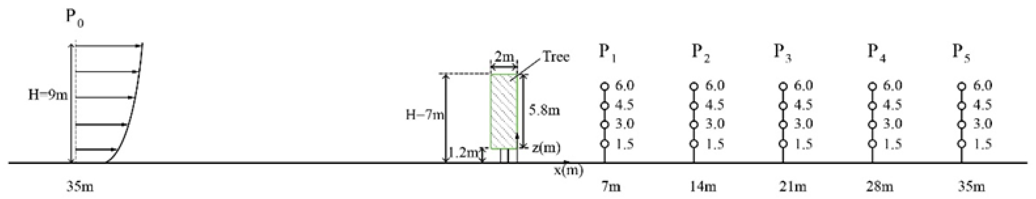
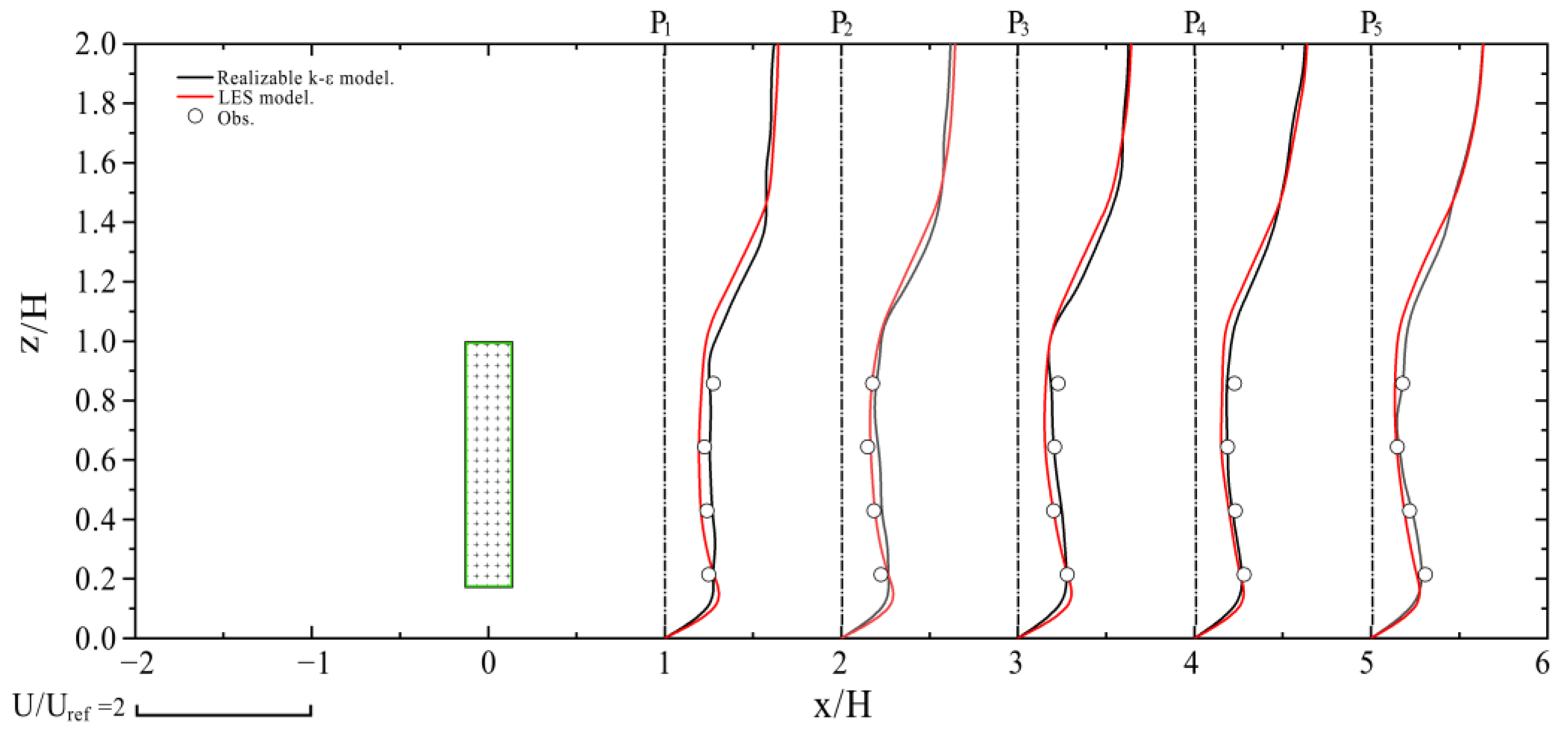
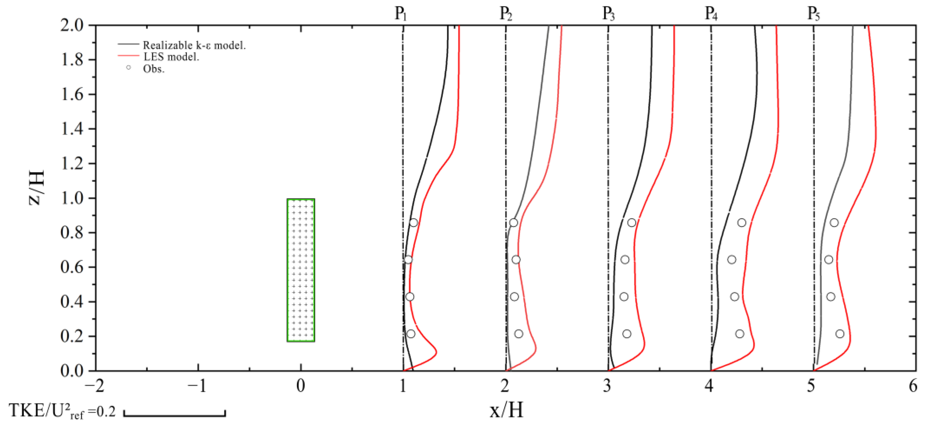
3.1. Validation of Numerical Method

Flow fields around the canopy model over the flat terrain were simulated by the realizable k–ε and LES model separately. The numerical results of these two models are compared with field measurement data for a row of trees in Izumo in order to validate the numerical method [41]. The length, width, and height of the canopy are 74 m, 2 m, and 7 m, respectively. The distance from the bottom of the leaf to the ground is 1.2 m. The inflow conditions were measured at 35 m upstream of the canopy at the heights of 1 m, 3 m, and 9 m. The mean wind speeds were measured at 7 m, 14 m, 21 m, 28 m, and 35 m leeward of the canopy at four different heights. The inflow wind direction was perpendicular to the canopy. The measurement was taken under neutral atmospheric conditions, which means that measurement data were not affected by local thermal effects. Figure 2 presents an illustration of the canopy model and measurement positions. Details of the testing of the canopy model simulations are given in Appendix B.

The mean wind speed profiles obtained from numerical results were compared with field measurement data, as shown in Figure 3. In general, the simulation results based on the two models are in good agreement with the measurement data, validating the accuracy of the numerical method. This may be attributed to the fact that the fluid force formula for the two models is the same, thus providing the same momentum loss in the simulation. An S-shape of the wind profiles was observed in both simulation results of the two models. This is mainly due to: (a) the increase in wind velocity at the top of the canopy; (b) the decrease in wind speed behind the canopy; and (c) insignificant acceleration at the bottom of the canopy. Additionally, the three phenomena result in strong shear stress at the top of the canopy. It can be observed from Figure 3 that, at x/H = 4 and x/H = 5, the differences between the two simulated cases are not substantial. However, in the case of x/H = 3, the numerical results with the realizable k–ε model are slightly more accurate than the LES model. The reason for this may be that the accurate prediction of the LES model depends largely on turbulent inflow conditions and grid resolution. Furthermore, their complexity requires the proper calibration of additional input parameters to produce reliable results.

The normalized turbulent kinetic energy profiles obtained from numerical results were compared with field measurement data, as shown in Figure 4. It can be observed that the simulated profiles by the realizable k–ε model in the wake region of the canopy are slightly underestimated in the range 2 < x/H < 4. However, in research on wind flow behind windbreaks, J.L. Santiago [2] concluded that the turbulence model could be considered acceptable under the condition that turbulent kinetic energy is underestimated. In addition, this paper aims to determine the optimum canopy structure giving rise to the largest shelter effect in order to protect the stone carvings, and the wind erosion mechanism discussed in Section 3.5 shows that the most effective way to mitigate the wind erosion of the historical stones is to reduce the average wind speed under the primary-harm wind direction. Therefore, this research mainly focuses on the mean flow characteristics around the shelterbelt. The average velocity profile simulated by the two models is similar to the measured data, so the performance of the realizable k–ε model is generally acceptable.

Compared with the LES model, the realizable k–ε turbulence model can better balance the computational accuracy and computational resources. Hence, the flow modeling through a windbreak in this study is based on realizable k–ε modeling of infinite dense canopy flow.

3.2. Influence of Canopy Internal Structural Parameter

In this section, the verified canopy model was applied to discuss the influence of canopy internal structure parameters on shelter efficiency. The most used parameter of canopy internal structure is porosity ($\mathsf{\alpha }$), which is a simple ratio of perforated area to total area. For thin artificial barriers, $\mathsf{\alpha }$is equivalent to optical porosity. However, optical porosity may not always satisfactorily describe the permeability of air flow because optical porosity shows only the two-dimensional gaps and cannot represent the three-dimensional spaces through which the wind flows across windbreaks with a certain width. The aerodynamic porosity, which describes the volume porosity, is a reasonable characterization parameter when the windbreak is a shelterbelt. Consequently, we have arbitrarily varied the value of ${\mathrm{C}}_{\mathrm{d}}\mathrm{A}\left(\mathrm{z}\right)$ and calculated the resulting aerodynamic porosity α. The aerodynamic porosity is defined as [42].

$$\mathsf{\alpha }=\frac{{\int }_{\mathrm{S}}^{}\mathrm{udS}}{{\int }_{\mathrm{S}}^{}{\mathrm{u}}_0\mathrm{dS}}$$

(3)

where u is the axial velocity component, ${\mathrm{u}}_0$ is the axial velocity component far upstream, and the integration is performed over vegetation canopy area S. The aerodynamic porosity is the ratio of the flow flux through the canopy cross section to the flow flux at the same cross-section far upstream.

To study the effect of the aerodynamic porosity on shelter efficiency, six cases with a value of ${\mathrm{C}}_{\mathrm{d}}\mathrm{A}\left(\mathrm{z}\right)$ = 0.4, 1.6, 3.2, 6.4, 9.6 and 25.6 were simulated. The respective calculated aerodynamic porosities α = 85, 57, 45, 35, 30, 18. Except for the vegetation canopy aerodynamic porosity introduced in the numerical simulation, all the other configuration parameters are identical to those in Section 3.1.

Figure 5 presents the contours of normalized mean wind speed around the canopy with different porosities in a cross-section of y/H = 0. As shown, the approach flow separates into two parts due to the canopy: displaced flow moves upward and passes over the canopy top, and bleed flow passes through the canopy pores. The mean wind speed decreases at the leeward of the windbreak because of the blockage effect created by the canopy. The larger the aerodynamic porosity, the less obvious the blockage effect is. As the porosity increases, the displaced flow speed gradually decreases. However, the bleed flow becomes stronger, inhibiting the formation of the quiet zone. For the sparse canopy (Figure 5a,b), the ambiguous region of the quiet zone simulated by the porous model is in agreement with an earlier study on the simulations of Poggia et al. [17] for a canopy with large porosity. Hence, the performance of the porous model describing the flow is acceptable.

As shown in Figure 5, maximum wind reductions are closely related to porosity, with low porosity producing high maximum reductions. The velocity along z/H = 1 has a U_ref = 0.8 down to 0.2 for aerodynamic porosities of 85–18% respectively. Barriers with very low porosity create increased turbulence downwind compared to the medium-dense vegetation canopy. The higher turbulence level may result in recovery of mean horizontal wind speeds to upwind speeds closer to the low-porosity vegetation canopy, thus resulting in a shorter protected distance.

The shelter efficiency of windbreaks are of great significance in their design. Over the years, many scholars have proposed several evaluation criteria, among which the most used are the distance d₂₀ over which wind speed is reduced by at least 20%, and the minimal wind speed U_min/U_ref on the leeward side of the windbreak and its location x_min [1]. The minimum relative wind speed U_min/U_ref may be of most interest where the area requiring protection is small. Since this paper mainly focuses on the average wind speed in front of the cave, U_min/U_ref is used as an index for the assessment of windbreak shelter efficiency.

Figure 5 also shows that the canopy with a porosity of 18–30% has the same value of U_min, whilst the canopy with a porosity of 30% has a larger value of d₂₀. This means that it can efficiently decrease downwind mean wind speed. Therefore, the optimal porosity of the canopy is 30%.

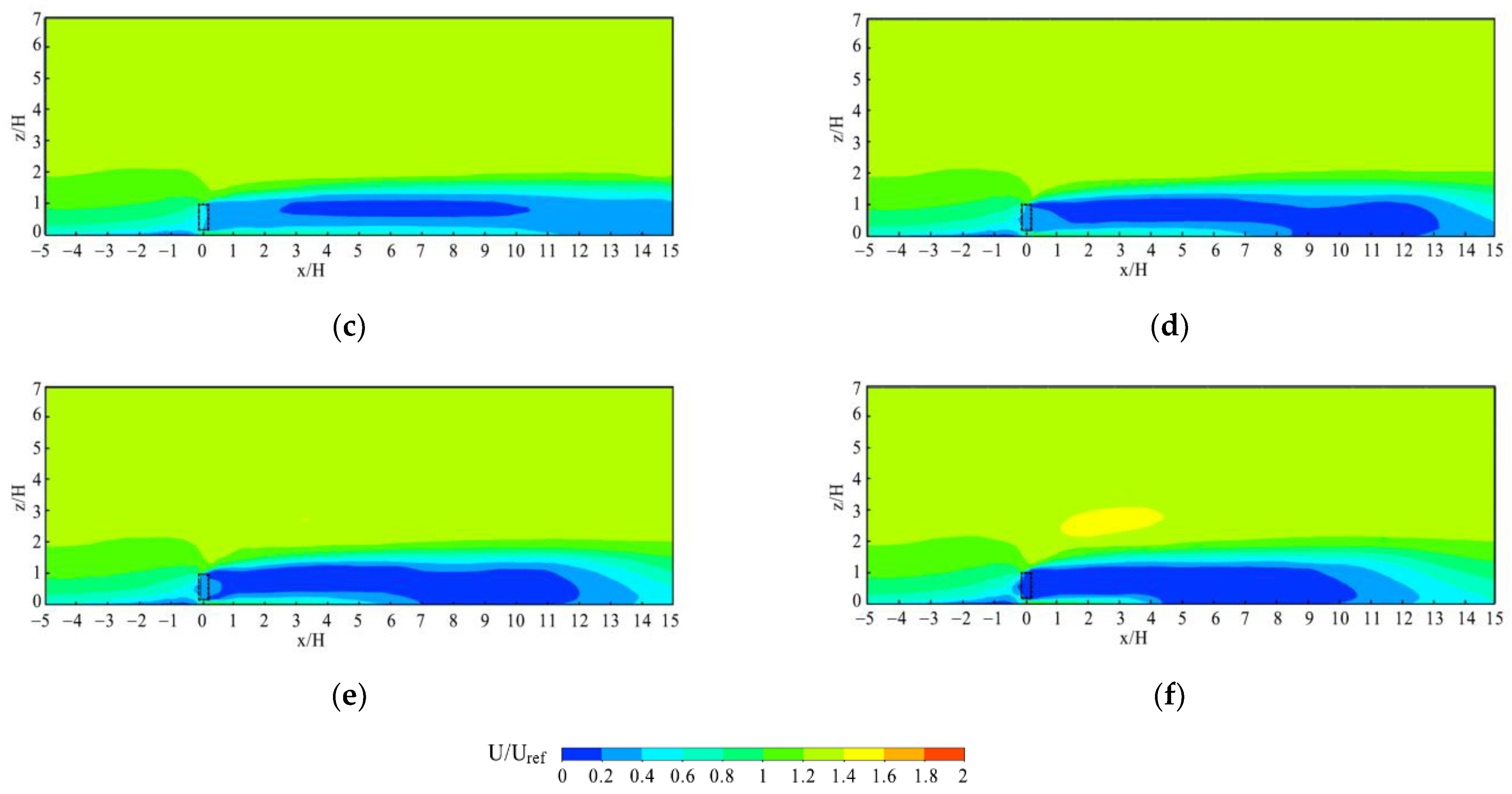
3.3. Influence of Canopy External Structural Parameter

Natural shelterbelts, unlike artificial fences, have a certain width. In this section, the flow fields around canopies of different widths are numerically studied, and their influences on shelter efficiency are discussed.

As described in Equations (2) and (A7), drag force per unit air mass and drag coefficient per unit LAD are local drag force and local drag coefficient of the shelterbelt, respectively. While total drag force of the entire shelterbelt is usually used in the research. For a two-dimensional artificial fence, the resistance coefficient or pressure-loss coefficient ${\mathrm{k}}_{\mathrm{r}}$ is the most used parameter to reflect aerodynamic properties of the entire windbreak. For the vegetation canopy, the value of ${\mathrm{k}}_{\mathrm{r}}$ may be roughly estimated as [43]:

$${\mathrm{k}}_{\mathrm{r}}={{\displaystyle \int }}_{-{\mathrm{w}}_{\mathrm{s}}}^0{\mathrm{C}}_{\mathrm{d}}\mathrm{A}\left(\mathrm{Z}\right)\mathrm{dx}$$

(4)

where ${\mathrm{w}}_{\mathrm{s}}$ is the width of the vegetation canopy.

We can see that ${\mathrm{k}}_{\mathrm{r}}$ is the integration of the product of local leaf-area density and the local dynamic property of leaf area along the i-direction, which relates the bulk aerodynamic property of the entire vegetation canopy to the local LAD and local drag coefficient. Therefore, for fixed values of ${\mathrm{k}}_{\mathrm{r}}$, a vegetation canopy with different widths has the same porosity. As listed in

Table 1. Parameters for cases with different widths.

Case No	1	2	3	4	5	6
Width (m)	0.1 H	0.3 H	0.5 H	1 H	2 H	3 H
$C_{d}A\left(Z\right)$ (m−1)	27.4	9.14	5.49	2.74	1.37	0.91

, there are six cases of vegetation canopies of spatially uniform ${\mathrm{C}}_{\mathrm{d}}\mathrm{A}\left(\mathrm{Z}\right)$ with different widths ranging from 0.1 H to 3 H. Except for the canopy with different widths introduced in the numerical simulation, all the other configuration parameters are identical to those in Section 3.1.

Figure 6 presents the contours of normalized mean wind speed around the canopy with different widths in the cross-section of y/H = 0. The width of the canopy significantly influences the perturbed flow fields on the leeside of the canopy and then affects the mean wind speed and the recovery of wind speed. For canopy width less than 1 H, the mean wind speed on the leeward side decreases as the width increases. However, for canopy width greater than 1 H, the variation tendency of mean wind speed on the leeward side is opposite to the above situation. When the width is between 0.3 H and 0.5 H, the canopy has the largest quiet zone area on the leeward side. When the width of the canopy is equal to 3 H, the flow above the canopy may completely adjust to the roughness of the canopy, so the characteristic of flow above and inside the plant canopy is heterogeneous.

As shown in Figure 6, the shelter efficiencies expressed in the minimal wind speed U_min/U_ref on the leeward side of the windbreak and its location x_min changes little for different widths. The principal reason for this is the compensation between the permeability and the downstream perturbed pressure of the canopy. In order to save forest resources, a width of 0.3 to 0.5 H for shelterbelts with a rectangular cross-section is suggested.

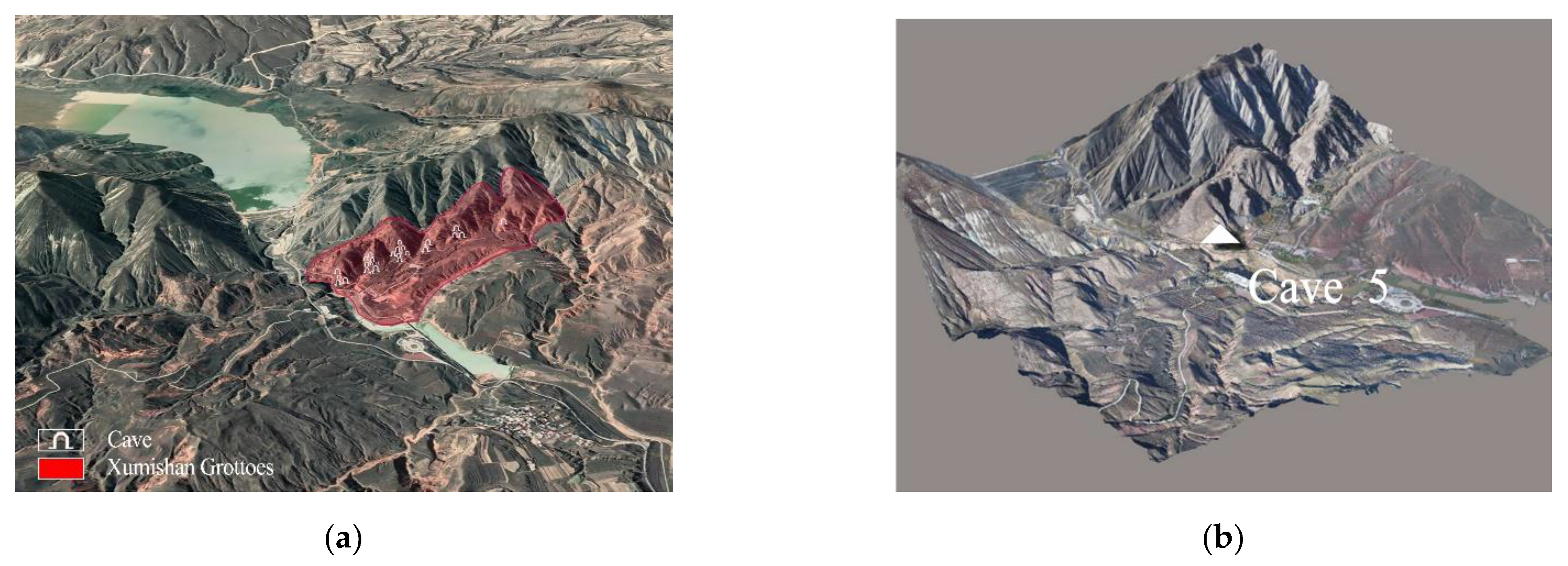
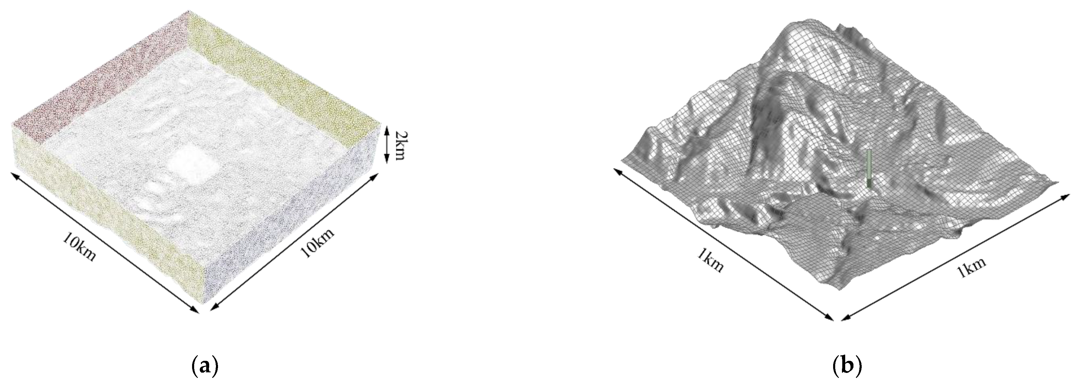
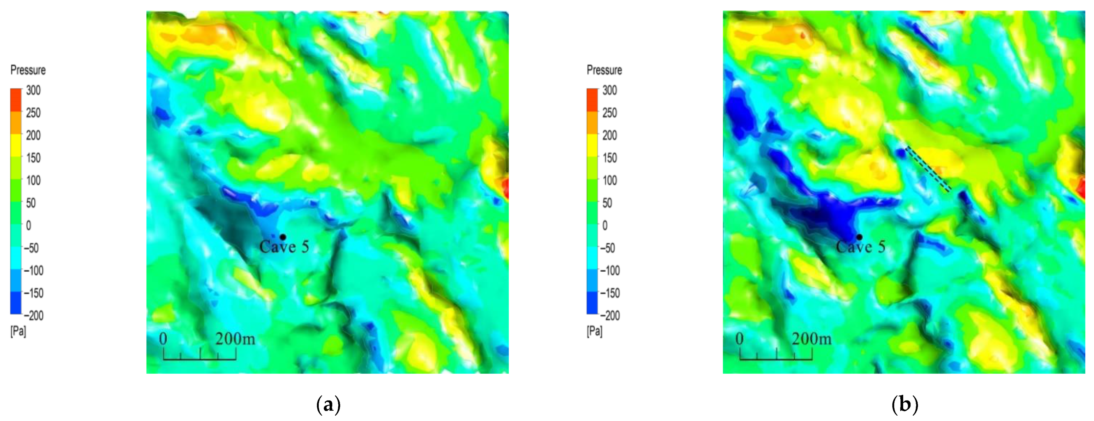
3.4. Flow Fields around Shelterbelt over a Real Complex Terrain

The Xumishan Grotto Zone is located at about 105°58′46″–105°59′21″ E, 36°16′13″–36°17′18″ N (Figure 7). Complex terrain is a generic term used in the literature to describe any irregular terrain. Grottoes in northwest China are often located in complex terrains such as cliffs and valleys. The Xumishan Grottoes, which are composed of valleys and hills with different elevations, are characterized by high levels of complexity. The caves of the Xumishan Grottoes are mainly distributed within a 1 km radius of Cave 5. Therefore, this paper focuses on microscale wind fields over complex terrain.

The numerical simulation of the flow fields is divided into two levels. At the higher level, in order to reflect the influence of upstream terrain on the wind flow characteristics [34], a terrain model with a horizontal resolution of 20 m within a 10 km × 10 km region is established based on a geographic information system (GIS) data (Figure 8). According to guidelines for CFD practices in wind engineering [44,45], the height of the computational domain is five times the maximum elevation difference in the region. Note that the height of the computational domain in this paper is similar to the atmospheric boundary layer height; the inflow turbulent kinetic energy and dissipation rate are different from those in Section 3.1, Section 3.2 and Section 3.3 and are formulated using Equations (5)–(8):

$$\mathrm{U}\left(\mathrm{z}\right)={\mathrm{U}}_{\mathrm{ref}}{(\frac{\mathrm{z}}{{\mathrm{z}}_{\mathrm{ref}}})}^{\mathsf{\alpha }}$$

(5)

$$\mathrm{k}\left(\mathrm{z}\right)={\left(\mathrm{U}\left(\mathrm{z}\right)·\mathrm{I}\left(\mathrm{z}\right)\right)}^2$$

(6)

$$\mathsf{\epsilon }\left(\mathrm{z}\right)={\mathrm{C}}_{\mathrm{u}}^{3/4}{\mathrm{k}}^{3/2}/\left({\mathsf{\kappa }}_{\mathrm{v}}\mathrm{z}\right)$$

(7)

$$\mathrm{I}\left(\mathrm{z}\right)=\{\begin{array}{l}0.1{({\mathrm{z}}_{\mathrm{b}}/{\mathrm{z}}_{\mathrm{G}})}^{-\mathsf{\alpha }-0.05} \mathrm{z}\le {\mathrm{z}}_{\mathrm{b}}\\ 0.1{(\mathrm{z}/{\mathrm{z}}_{\mathrm{G}})}^{-\mathsf{\alpha }-0.05} {\mathrm{z}}_{\mathrm{b}}<\mathrm{z}\le {\mathrm{z}}_{\mathrm{G}}\\ 0.1 \mathrm{z}>{\mathrm{z}}_{\mathrm{G}}\end{array}$$

(8)

where ${\mathrm{z}}_{\mathrm{ref}}$ and ${\mathrm{U}}_{\mathrm{ref}}$ are the standard reference height and standard reference wind speed set to 10 m and 10 m/s in this paper, respectively. The fitting result for the profile index α is 0.26 according to the drone field test wind profile. The corresponding gradient wind height is 400 m, which means wind speed no longer increases with the distance from the ground.

The Grotto Zone in this study is 1 × 1 km², and a horizontal resolution of 5 m within this region was established through drone oblique photogrammetry at the current level. The wind characteristics (including the velocity profile, turbulent kinetic energy profile, and dissipation rate profile) of the higher-level simulation are used as the inlet boundary conditions of the current-level simulation [46,47] (Figure 9).

In order to validate the simulation accuracy, the simulated flow in the complex terrain around the caves was compared with local meteorological data. The Huangduobao meteorological station (MS1) is located northeast of this region, and it was located upstream of the prevailing wind direction as a reference. The meteorological station of the Xumishan Grottoes (MS2) is located in the center of the area and can accurately monitor the wind climate around Cave 5. The location of meteorological stations can be seen in Figure 10. The simulated values are in black, the measured values are in red, and the wind direction standard deviation of the measured values is in red.

Figure 11 shows a comparison between the simulated and measured values of wind speed ratio and wind direction at Xumishan Grottoes meteorological station. The numerical values of wind speed are generally within 25% of the corresponding measurements, and the maximum difference value of the wind direction is less than 20%. The results show that the method can accurately simulate the spatial wind field of complex terrain.

Pinus is a common, tall tree planted in the study area. It is a pine evergreen coniferous tree with an average height in its forests up to 30 m. This height was used as the canopy height. Based on the previous discussion, the optimum vegetation canopy structure was confirmed to provide a guideline for designing a shelterbelt. In this simulation, the porosity of the canopy was 30%, and the width was 0.4 H. For natural barriers, as the approach angle (the angle of average wind direction from perpendicular to the windbreak) increases, the effective porosity of the windbreak becomes smaller. The shelter efficiency of a canopy is a function of approach angle and porosity. Medium-dense (φ = 30%) canopy reaches a maximum shelter efficiency with the approach angle value of 90°. The distance between windbreaks and shelterbelt is about 3 H. At this distance, the wind speed is reduced to the minimum value in the approach flow.

Figure 12 presents the contours of normalized mean wind speed around the shelterbelt over complex terrain in a cross-section perpendicular to the canopy. It can be found that flow characteristics downwind of the shelterbelt are obviously different in various inflow directions. When the inflow direction is northeast, the quiet zone region on the leeward side of the canopy is significantly reduced, indicating that the disturbance from the downstream hills may still affect the flow. When the inflow direction is southwest, the downwind terrain of the shelterbelt is relatively flat, and the upstream hills have little influence on flow characteristics.

Figure 13 shows the streamline behind the shelterbelt over complex terrain. The flow fields are significantly affected by the geomorphic features of the terrain. When the inflow direction is in the northeast, due to the blocking effect of the downstream hills, the airflow accelerates between the shelterbelt and the hills. The wind speed on the leeward side of the shelterbelt increases gradually as the slope increases and reaches the maximum value at the ridge, which also explains why the quiet zone region on the leeward side of the canopy decreases significantly in Figure 13a. When the inflow direction is southwest, the flow characteristics downwind of the shelterbelt are less affected by topography. The flow separation phenomenon occurs in the area near the leeward side, and a vortex is also generated.

It can be seen from the simulation results that terrain features are an important factor affecting the flow characteristics, and the downstream hills have a large influence on the flow characteristics in the quiet zone of the shelterbelt. In order to make sure that the simulated flow fields’ flow characteristics are closer to the real, it is necessary to take turbulent flow, influenced by the leeside of the actual hill and the presence of the shelterbelt, into comprehensive consideration.

3.5. Relationship between Local Wind Conditions and Wind Erosion

Cave 5, which this paper focuses on, is representative of the Tang Dynasty statues in the Xumishan Grottoes. The feet of the Buddha statue in the Grottoes have been eroded by strong winds into the honeycomb caves (Figure 14a,b).

Figure 15 shows the contours of the simulated wind speed ratio in the horizontal plane at Cave 5 height under eight wind directions without a shelterbelt. When the inlet wind direction is northeast (Figure 15a), the inflow direction is close to the trend of the valley channel, and the wind speed around Cave 5 is less blocked by the mountain. Another reason for this is that as the airflow from the open area to the channel terrain, it accelerates through and forms a high-speed canyon wind. For these reasons, the wind speed amplification coefficient reaches the maximum value of 2.1. When the angle between the inlet wind direction and the river channel increases, the wind speed in front of the cave decreases significantly, and the mountain barrier effect is obvious. When the wind direction is northwest (Figure 15g), the wind speed in front of the cave on the leeward side of the mountain reaches the lowest value due to the blocking effect of the mountain on the northwest side and the wind speed amplification coefficient is 0.3.

Figure 16 shows the angle of attack (AOA) around Cave 5 when the inlet wind direction is northeast (Figure 16a), and the calculated values of AOA range between −5° and 10°, illustrating that wind characteristics are associated with lower turbulence level. If the inlet wind direction is northwest (Figure 16g), the calculated values of AOA range between −15° and 20°. The significant change in AOA indicates that turbulence increases locally. In general, the angle of attack is positive on the upslope and negative on the downslope. Combined with the terrain slope, it is found that the position with a larger angle of attack corresponds to a larger slope. Additionally, an angle of attack close to or above 15° reflects flow separations, especially in downslope flow. The angle of attack changes suddenly for the northwest flow attributed to Cave 5 located at the leeward wall of the valley, resulting in a recirculation zone around Cave 5. The flow near mountain surfaces tends to travel vertically, and near-ground flow travels opposite to the inlet wind direction.

The simulation results showed that Cave 5, being located in low wind speed areas, is associated with increased 3D turbulence of the northwest flow, and strong wind speed is associated with lower turbulence of the northeast flow. When the wind approaches from the northwest, the wind velocity and turbulence level in this characteristic wake region are significantly affected by the presence of the mountain. The shelter effect results in a region of low-speed flow beneath the mountain height and an increased turbulence level experienced at approximately the height of the mountain. When the wind approaches from the northeast, the effect of the mountain on the wake region is reduced, and flow with lower turbulence and high speed is observed.

Figure 17a shows the contours of the hill surface pressure distribution in the absence of a shelterbelt: the flow separations lead to a negative pressure value at the ridge and the leeside pressure increases gradually. The value of pressure around Cave 5 is −95 Pa. Figure 17b shows the contours of the hill and canopy surface pressure distribution with the influence of the shelterbelt. We can see that the pressure is significantly affected by the presence of the shelterbelt. The shelterbelt behaves in a similar way to an obstacle, increasing the pressure substantially at the windward side of the shelterbelt, forming a large area of positive pressure area. During the displaced flow through the shelterbelt, a larger negative pressure area is generated on the leeward side, and a region characterized by low turbulence is generated due to the reversed flow. The value of pressure around Cave 5 is −150 Pa. The reduction of pressure on the stone-surface is beneficial to the protection of carving to a certain extent.

The deterioration of the Xumishan Grottoes is the long-term result of this, and wind blowing and rotary grinding are the main causes of wind erosion. Under the conditions of blowing and rotary grinding, the surface of the rock mass is mainly affected by pressures and wind velocity. Woodruff, N.P, first proposed a wind erosion equation that is widely used around the world [48]. The wind erosion climate factor index C, one of the five variables of the equation, is used to represent the influence of climate conditions on the wind erosion degree. The wind erosion climate factor index is given by [49]:

$$\mathrm{C}=\frac{1}{100}{{\displaystyle \sum }}_{\mathrm{i}=1}^{12}{\overline{\mathrm{u}}}^3\left(\frac{{\mathrm{ETP}}_{\mathrm{i}}-{\mathrm{P}}_{\mathrm{i}}}{{\mathrm{ETP}}_{\mathrm{i}}}\right)\mathrm{d}$$

(9)

where C is the wind erosion climatic factor index, $\overline{\mathrm{u}}$ is the monthly average wind speed (m/s) at 2 m, ${ \mathrm{P}}_{\mathrm{i}}$ is the monthly precipitation (mm), ET${\mathrm{P}}_{\mathrm{i}}$ is the monthly potential evaporation (mm), and d is the number of days in a month.

Figure 18 shows the contours of the simulated wind speed ratio with the effect of the shelterbelt. The shelterbelt generates a clear wake region behind itself and shows a quite different mean wind speed compared to the upstream region. Regarding the wind velocity, when the inlet direction is the primary-harm wind direction (Figure 18a), the wind speed amplification coefficient around Cave 5 decreases to 1.2. Compared to the case with no shelterbelt, the wind speed amplification coefficient decreased by 43%. The significant decrease in this value in the primary-harm wind direction demonstrates the effectiveness of the shelterbelt. Since the shelterbelt is modeled as a porous medium, the compensation between the effects of permeability and perturbed pressure results in the lack of recirculating eddies in the immediate lee, with decreased turbulence. Thus, Cave 5 can be located in areas with decreased 3D turbulence and low wind speed. It is, therefore, effective to use the shelterbelt to decrease the degree of wind erosion on stone carvings in this area. This conclusion can be used to guide how to adjust the wind field near the caves by setting up reasonable passive technologies such as the shelterbelt in the Grotto Zone and provides guidance for solving the problem of stone carving erosion caused by strong wind erosion in semi-open Grottoes to achieve preventive protection of stone carvings in these areas.

4. Conclusions

Based on the RANS equation and realizable k–ε model, flow fields over complex terrain are investigated in this paper. The main conclusions are summarized as follows:

The canopy model combined with the realizable k–ε turbulence model can accurately simulate the flow fields around vegetation. The results have shown that the canopy model has a good performance on parameterizations of aerodynamic effects of trees via CFD simulations.

The interaction of penetrating flow with the perturbation pressure and displace flows over the canopy creates a maximum wind speed reduction downstream of the canopy. The results show that a canopy with porosity of φ = 30% and a width of 0.3 H to 0.5 H has a better shelter efficiency. Therefore, the resulting flow fields around the canopy also provided quantitative information to help in the assessment of designing shelterbelt and the effect of vegetative windbreak on alleviating the wind erosion degree of stone carvings.

Terrain features are an important factor affecting flow characteristics, and the downstream hills have a large influence on the flow characteristics in the quiet zone of the shelterbelt. In order to make sure that the simulated flow fields are similar to the real flow characteristics, it is necessary to take turbulent flow that is influenced by the leeside of the actual hill and the presence of the shelterbelt into comprehensive consideration.

The significant decrease in this value in the primary-harm wind direction demonstrates the effectiveness of the shelterbelt. Since the shelterbelt is modeled as a porous medium, the compensation between the effects of permeability and perturbed pressure results in the lack of recirculating eddies in the immediate lee, with decreased turbulence. Thus, Cave 5 can be located in areas with decreased 3D turbulence and low wind speed. It is, therefore, effective to use the shelterbelt to decrease the degree of wind erosion on stone carvings in this area. This conclusion can be used to guide how to adjust the wind field near the caves in the Grotto Zone and provides guidance for solving the problem of stone carving erosion caused by strong wind in order to achieve preventive protection of stone carvings in the Grottoes.

References

1. Heisler, G.M.; Dewalle, D.R. Effects of Windbreak Structure on Wind Flow. Agric. Ecosyst. Environ. 1988, 22, 41–69. [Google Scholar] [CrossRef]
2. Santiago, J.L.; Martín, F.; Cuerva, A.; Bezdenejnykh, N.; Sanz-Andrés, A. Experimental and Numerical Study of Wind Flow behind Windbreaks. Atmos. Environ. 2007, 41, 6406–6420. [Google Scholar] [CrossRef] [Green Version]
3. Buccolieri, R.; Santiago, J.-L.; Rivas, E.; Sanchez, B. Review on Urban Tree Modelling in CFD Simulations: Aerodynamic, Deposition and Thermal Effects. Urban For. Urban Green. 2018, 31, 212–220. [Google Scholar] [CrossRef]
4. Chen, G.; Wang, W.; Sun, C.; Li, J. 3D Numerical Simulation of Wind Flow behind a New Porous Fence. Powder Technol. 2012, 230, 118–126. [Google Scholar] [CrossRef]
5. Shang, R.; Yan, Z.; Wang, X.; Zhang, Z.; Gao, W. Research on the Wind Environment of the Landscape Forest Belts in Front of Dunhuang Mogao Grottoes. GAK 2016, 69, 752–760. [Google Scholar]
6. Shang, R.; Yan, Z.; Wang, X.; Zhang, Z.; Wang, J.; Fan, X.; Gao, W. Research on the Micro-Climate Environment of Mogao Grottoes. Dunhuang Res. 2016, 35, 117–123. [Google Scholar]
7. Cornelis, W.M.; Gabriels, D.; Lauwaerts, T. Simulation of Windbreaks for Wind-Erosion Control in a Wind Tunnel. 1997. Available online: http://www.researchgate.net/publication/268052845 (accessed on 1 April 2022).
8. Wang, H.; Takle, E.S. Momentum Budget and Shelter Mechanism of Boundary-Layer Flow near a Shelterbelt. Bound.-Layer Meteorol. 1997, 82, 417–437. [Google Scholar] [CrossRef]
9. Wilson, J.D. A Second-Order Closure Model for Flow through Vegetation. Bound.-Layer Meteorol. 1988, 42, 371–392. [Google Scholar] [CrossRef]
10. Krayenhoff, E.S.; Santiago, J.-L.; Martilli, A.; Christen, A.; Oke, T.R. Parametrization of Drag and Turbulence for Urban Neighbourhoods with Trees. Bound.-Layer Meteorol. 2015, 156, 157–189. [Google Scholar] [CrossRef]
11. Santiago, J.-L.; Rivas, E.; Sanchez, B.; Buccolieri, R.; Martin, F. The Impact of Planting Trees on NOx Concentrations: The Case of the Plaza de La Cruz Neighborhood in Pamplona (Spain). Atmosphere 2017, 8, 131. [Google Scholar] [CrossRef] [Green Version]
12. Wang, H.; Takle, E.S. On Three-Dimensionality of Shelterbelt Structure and Its Influences on Shelter Effects. Bound.-Layer Meteorol. 1996, 79, 83–105. [Google Scholar] [CrossRef]
13. Fang, F.-M.; Chang, J.-C.; Li, Y.-C.; Chung, C.-Y.; Chan, M.-H. Shelter Effect of Pedestrian Wind behind Row Trees in a Line Arrangement. Forests 2022, 13, 392. [Google Scholar] [CrossRef]
14. Santiago, J.-L.; Rivas, E. Advances on the Influence of Vegetation and Forest on Urban Air Quality and Thermal Comfort. Forests 2021, 12, 1133. [Google Scholar] [CrossRef]
15. Finnigan, J.J.; Belcher, S.E. Flow over a Hill Covered with a Plant Canopy. Q. J. R. Meteorol. Soc. 2004, 130, 1–29. [Google Scholar] [CrossRef] [Green Version]
16. Katul, G.G.; Finnigan, J.J.; Poggi, D.; Leuning, R.; Belcher, S.E. The Influence of Hilly Terrain on Canopy-Atmosphere Carbon Dioxide Exchange. Bound.-Layer Meteorol. 2006, 118, 189–216. [Google Scholar] [CrossRef]
17. Poggi, D.; Katul, G.G. Turbulent Flows on Forested Hilly Terrain: The Recirculation Region. Q. J. R. Meteorol. Soc. 2007, 133, 1027–1039. [Google Scholar] [CrossRef]
18. Dupont, S.; Brunet, Y.; Finnigan, J.J. Large-Eddy Simulation of Turbulent Flow over a Forested Hill: Validation and Coherent Structure Identification. Q. J. R. Meteorol. Soc. 2008, 134, 1911–1929. [Google Scholar] [CrossRef]
19. Jessie, P.B.; In-Bok, L.; Hyun-Seob, H.; Myeong-Ho, S. Numerical Simulation Study of a Tree Windbreak. Biosyst. Eng. 2012, 111, 40–48. [Google Scholar] [CrossRef]
20. Miri, A.; Dragovich, D.; Dong, Z. Wind Flow and Sediment Flux Profiles for Vegetated Surfaces in a Wind Tunnel and Field-Scale Windbreak. CATENA 2021, 196, 104836. [Google Scholar] [CrossRef]
21. Judd, M.J.; Raupach, M.R.; Finnigan, J.J. A Wind Tunnel Study of Turbulent Flow around Single and Multiple Windbreaks, Part I: Velocity Fields. Bound.-Layer Meteorol. 1996, 80, 127–165. [Google Scholar] [CrossRef]
22. Středová, H.; Podhrázská, J.; Litschmann, T.; Středa, T.; Rožnovský, J. Aerodynamic Parameters of Windbreak Based on Its Optical Porosity. Contrib. Geophys. Geod. 2012, 42, 213–226. [Google Scholar] [CrossRef]
23. He, Y.; Jones, P.J.; Rayment, M. A Simple Parameterisation of Windbreak Effects on Wind Speed Reduction and Resulting Thermal Benefits to Sheep.Pdf. Agric. Meteorol. 2017, 239, 96–107. [Google Scholar] [CrossRef] [Green Version]
24. Schwartz, R.C.; Fryrear, D.W.; Harris, B.L.; Bilbro, J.D.; Juo, A.S.R. Mean Flow and Shear Stress Distributions as Influenced by Vegetative Windbreak Structure. Agric. Meteorol. 1995, 75, 1–22. [Google Scholar] [CrossRef]
25. Desmond, C.J.; Watson, S.J.; Hancock, P.E. Modelling the Wind Energy Resource in Complex Terrain and Atmospheres. Numerical Simulation and Wind Tunnel Investigation of Non-Neutral Forest Canopy Flow. J. Wind Eng. Ind. Aerod. 2017, 166, 48–60. [Google Scholar] [CrossRef] [Green Version]
26. Hong, S.-W.; Lee, I.-B.; Seo, I.-H. Modelling and Predicting Wind Velocity Patterns for Windbreak Fence Design. J. Wind Eng. Ind. Aerod. 2015, 142, 53–64. [Google Scholar] [CrossRef]
27. Desmond, C.J.; Watson, S.J.; Aubrun, S.; Ávila, S.; Hancock, P.; Sayer, A. A Study on the Inclusion of Forest Canopy Morphology Data in Numerical Simulations for the Purpose of Wind Resource Assessment. J. Wind Eng. Ind. Aerod. 2014, 126, 24–37. [Google Scholar] [CrossRef] [Green Version]
28. Gromke, C.; Buccolieri, R.; Di Sabatino, S.; Ruck, B. Dispersion Study in a Street Canyon with Tree Planting by Means of Wind Tunnel and Numerical Investigations—Evaluation of CFD Data with Experimental Data. Atmos. Environ. 2008, 42, 8640–8650. [Google Scholar] [CrossRef]
29. Santiago, J.-L.; Buccolieri, R.; Rivas, E.; Calvete-Sogo, H.; Sanchez, B.; Martilli, A.; Alonso, R.; Elustondo, D.; Santamaría, J.M.; Martin, F. CFD Modelling of Vegetation Barrier Effects on the Reduction of Traffic-Related Pollutant Concentration in an Avenue of Pamplona, Spain. Sustain. Cities Soc. 2019, 48, 101559. [Google Scholar] [CrossRef]
30. Buccolieri, R.; Santiago, J.L.; Martilli, A. CFD Modelling: The Most Useful Tool for Developing Mesoscale Urban Canopy Parameterizations. Build. Simul. 2021, 14, 407–419. [Google Scholar] [CrossRef]
31. Mochida, A.; Tabata, Y.; Iwata, T.; Yoshino, H. Examining Tree Canopy Models for CFD Prediction of Wind Environment at Pedestrian Level. J. Wind Eng. Ind. Aerod. 2008, 96, 1667–1677. [Google Scholar] [CrossRef]
32. Blocken, B. 50 Years of Computational Wind Engineering: Past, Present and Future. J. Wind Eng. Ind. Aerod. 2014, 129, 69–102. [Google Scholar] [CrossRef]
33. Blocken, B. Computational Fluid Dynamics for Urban Physics: Importance, Scales, Possibilities, Limitations and Ten Tips and Tricks towards Accurate and Reliable Simulations. Build. Environ. 2015, 91, 219–245. [Google Scholar] [CrossRef] [Green Version]
34. Blocken, B.; vander Hout, A.; Dekker, J.; Weiler, O. CFD Simulation of Wind Flow over Natural Complex Terrain: Case Study with Validation by Field Measurements for Ria de Ferrol, Galicia, Spain. J. Wind Eng. Ind. Aerod. 2015, 147, 43–57. [Google Scholar] [CrossRef]
35. Li, J.; Liu, J.; Srebric, J.; Hu, Y. The Effect of Tree-Planting Patterns on the Microclimate within a Courtyard.Pdf. Sustainability. 2019, 11, 1665. [Google Scholar] [CrossRef] [Green Version]
36. Taleb, H.M.; Kayed, M. Applying Porous Trees as a Windbreak to Lower Desert Dust Concentration: Case Study of an Urban Community in Dubai. Urban For. Urban Green. 2021, 57, 126915. [Google Scholar] [CrossRef]
37. Shih, T.-H.; Liou, W.W.; Shabbir, A.; Yang, Z.; Zhu, J. A New K-ϵ Eddy Viscosity Model for High Reynolds Number Turbulent Flows. Comput. Fluids. 1995, 24, 227–238. [Google Scholar] [CrossRef]
38. Qi, Y.; Ishihara, T. Numerical Study of Turbulent Flow Fields around of a Row of Trees and an Isolated Building by Using Modified K–ε Model and LES Model. J. Wind Eng. Ind. Aerod. 2018, 177, 293–305. [Google Scholar] [CrossRef]
39. Bailey, B.N.; Stoll, R. Turbulence in Sparse, Organized Vegetative Canopies: A Large-Eddy Simulation Study. Bound.-Layer Meteorol. 2013, 147, 369–400. [Google Scholar] [CrossRef]
40. Lopes, A.S.; Palma, J.M.L.M.; Lopes, J.V. Improving a Two-Equation Turbulence Model for Canopy Flows Using Large-Eddy Simulation. Bound.-Layer Meteorol. 2013, 149, 231–257. [Google Scholar] [CrossRef]
41. Kurotani, Y.; Kiyota, N.; Kobayashi, S. Windbreak Effect of Tsuijimatsu in Izumo:Part. 2. Proc. Archit. Inst. Jpn. 2001, 745–746. [Google Scholar]
42. Guan, D.; Zhang, Y.; Zhua, T. A Wind-Tunnel Study of Windbreak Drag.Pdf. Agric. Meteorol. 2003, 118, 75–84. [Google Scholar] [CrossRef]
43. Wilson, J.D. Numerical Studies of Flow through a Windbreak. J. Wind Eng. Ind. Aerod. 1985, 21, 119–154. [Google Scholar] [CrossRef]
44. Franke, J.; Hellsten, A.; Schlunzen, K.H.; Carissimo, B. The COST 732 Best Practice Guideline for CFD Simulation of Flows in the Urban Environment: A Summary. Int. J. Environ. Pollut. 2011, 44, 419–427. [Google Scholar] [CrossRef]
45. Tominaga, Y.; Mochida, A.; Yoshie, R.; Kataoka, H.; Nozu, T.; Yoshikawa, M.; Shirasawa, T. AIJ Guidelines for Practical Applications of CFD to Pedestrian Wind Environment around Buildings. J. Wind Eng. Ind. Aerod. 2008, 96, 1749–1761. [Google Scholar] [CrossRef]
46. Li, C.; Zhou, S.; Xiao, Y.; Huang, Q.; Li, L.; Chan, P.W. Effects of Inflow Conditions on Mountainous/Urban Wind Environment Simulation. Build. Simul. 2017, 10, 573–588. [Google Scholar] [CrossRef]
47. Yamada, T.; Koike, K. Downscaling Mesoscale Meteorological Models for Computational Wind Engineering Applications. J. Wind Eng. Ind. Aerod. 2011, 99, 199–216. [Google Scholar] [CrossRef]
48. Woodruff, N.P.; Siddoway, F.H. A Wind Erosion Equation. Soil Sci. Soc. Am. J. 1965, 29, 602–608. [Google Scholar] [CrossRef]
49. FAO. A Provisional Methodology for Soil Degradation Assessment; FAO: Rome, Italy, 1979. [Google Scholar]
50. Sanz, C. A Note on k–ε Modelling of Vegetation Canopy Air-Flows. Bound.-Layer Meteorol. 2003, 108, 191–197. [Google Scholar] [CrossRef]
51. Sogachev, A.; Panferov, O. Modification of Two-Equation Models to Account for Plant Drag. Bound.-Layer Meteorol. 2006, 121, 229–266. [Google Scholar] [CrossRef]
52. Blocken, B.; Stathopoulos, T.; Carmeliet, J. CFD Simulation of the Atmospheric Boundary Layer: Wall Function Problems. Atmos. Environ. 2007, 41, 238–252. [Google Scholar] [CrossRef]
53. Richards, P. Appropriate Boundary Conditions for Computational Wind Engineering Models Using the K–ε Turbulence Model. J. Wind Eng. Ind. Aerod. 1993, 46, 145–153. [Google Scholar] [CrossRef]
54. Enoki, K.; Ishihara, T. A generalized canopy model and its application to the prediction of urban wind climate. Agric. Ecosyst. Environ. 2012, 68, 28–47. [Google Scholar] [CrossRef] [Green Version]
Figure 1. Schematic diagram of flow field around a windbreak. The areas with different colors in the figure indicate different regions mentioned in the text. The lines and arrows indicate streamlines around the windbreak. (Adapted from Judd et al.) [21].
Forests 13 01072 g001
Figure 2. Configuration of canopy and measurement positions in the field measurement.
Forests 13 01072 g002
Figure 3. Comparison of simulated and measured profiles of mean wind speed behind the row of canopy. The green rectangular marks the canopy region occupied by trees.
Forests 13 01072 g003
Figure 4. Comparison of simulated and measured profiles of turbulent kinetic energy behind the row of canopy. The green rectangular marks the canopy region occupied by trees.
Forests 13 01072 g004
Figure 5. Normalized mean wind speed around the canopy with different porosities in cross section of y/H = 0, (a) φ = 85%, (b) φ = 58, (c) φ = 46, (d) φ = 35, (e) φ = 30, (f) φ = 18. The dotted line rectangular marks the canopy region occupied by trees.
Forests 13 01072 g005aForests 13 01072 g005b
Figure 6. Normalized mean wind speed around the canopy with different widths in cross section of y/H = 0, (a) W = 0.1 H, (b) W = 0.3 H, (c) W = 0.5 H, (d) W = 1 H, (e) W = 2 H, (f) W = 3 H. The dotted line rectangular marks the canopy region occupied by trees.
Forests 13 01072 g006aForests 13 01072 g006b
Figure 7. (a) Perspective view from the east, where red is the Grotto Zone, (b) topography map of the focused terrain.
Forests 13 01072 g007
Figure 8. Computational domain (a) higher-level domain. (b) current-level domain.
Forests 13 01072 g008
Figure 9. Computational domains (a): Domain 1 is the higher-level domain. Domain 2 is the current-level domain. Dashed lines indicate interface of wind characteristics interpolated to the current-level. Elevation information of Domain 2 (b).
Forests 13 01072 g009
Figure 10. Colour contours of the simulated and measured wind speed ratio at 10 m height above ground (a) 67.5°; (b) 90°; (c) 112.5°; (d) 135°.
Forests 13 01072 g010
Figure 11. Comparison of the simulated and measured (a) wind speed ratio; (b) wind direction. The red dot indicates four different reference wind directions.
Forests 13 01072 g011
Figure 12. Normalized mean wind speed around the shelterbelt over complex terrain (a) Northeast direction; (b) southwest direction.
Forests 13 01072 g012
Figure 13. Streamline behind the shelterbelt over complex terrain (a) Northeast direction; (b) southwest direction.
Forests 13 01072 g013
Figure 14. (a) Buddha statue in Cave 5; (b) wind erosion symptoms of Buddha foot.
Forests 13 01072 g014
Figure 15. Contours of the simulated wind speed ratio in a horizontal plane at Cave 5 height for the inlet wind directions of 45°–360°. (a) 45°; (b) 90°; (c) 135°; (d) 180°; (e) 225°; (f) 270°; (g) 315°; (h) 360°.
Forests 13 01072 g015
Figure 16. Colour contours of the angle of attack around Cave 5 for the inlet wind directions of 45°–360°. (a) 45°; (b) 90°; (c) 135°; (d) 180°; (e) 225°; (f) 270°; (g) 315°; (h) 360°.
Forests 13 01072 g016aForests 13 01072 g016b
Figure 17. Contours of the simulated pressure around Cave 5 for the inlet wind directions of 45°, (a) without shelterbelt; (b) with shelterbelt. The rectangular in black line represents the position of shelterbelt.
Forests 13 01072 g017
Figure 18. Contours of the simulated wind speed ratio in a horizontal plane at Cave 5 height with the influence of shelterbelt for the inlet wind directions of 45°–360°. The rectangular in black line represents the position of shelterbelt. (a) 45°; (b) 90°; (c) 135°; (d) 180°; (e) 225°; (f) 270°; (g) 315°; (h) 360°.
Forests 13 01072 g018aForests 13 01072 g018b