Article

Response of Spruce Forest Ecosystem CO2 Fluxes to Inter-Annual Climate Anomalies in the Southern Taiga

1
A.N. Severtsov Institute of Ecology and Evolution, Russian Academy of Sciences, Leninsky Prospect 33, 119071 Moscow, Russia
2
Faculty of Geography, M.V. Lomonosov Moscow State University, GSP-1, Leninskie Gory, 119991 Moscow, Russia
*
Author to whom correspondence should be addressed.
Forests 2022, 13(7), 1019; https://doi.org/10.3390/f13071019
Submission received: 25 May 2022 / Revised: 26 June 2022 / Accepted: 27 June 2022 / Published: 29 June 2022
(This article belongs to the Special Issue Soil Organic Matter and Nutrient Cycling in Forests)

Abstract

:
Climate extremes and anomalies modify the CO2 ecosystem–atmosphere exchange of the boreal forests and consequently alter the terrestrial carbon stocks and the atmospheric greenhouse gas concentrations. The effects of the anomalous weather conditions on the CO2 net ecosystem exchange (NEE), total ecosystem respiration (TER), and gross primary production (GPP) of the typical southern taiga nemorose spruce forest were analyzed using continuous eddy covariance flux measurements in the 2015–2020 period. The forest was found to be a source of atmospheric CO2 in 2016, 2017, 2019, and 2020 (the mean annual GPP/TER ratio was between 0.87 and 0.97). In 2018, the forest was found to act as a CO2 sink (GPP/TER = 1.47) when a positive temperature anomaly in the growing season was accompanied by a negative precipitation anomaly and increased global radiation. The early start of the CO2 uptake in the anomalously warm winter of 2019/2020 did not result in an increase in the annual GPP/TER ratio (0.90). The comparison of the flux data obtained from the nemorose spruce forest on the well-drained soils with the data obtained from paludified spruce forest in the same landscape showed that the mean annual GPP/TER ratio of the sites alternatively responded to the mentioned anomalies. This study suggests that a variety of soil moisture regimes across the southern taiga spruce forests provide a non-uniformity in the response reactions of the CO2 ecosystem–atmosphere exchange on the climate anomalies.

1. Introduction

Boreal forests constitute about one-third of the mean global terrestrial carbon sink and are the major contributors to the global terrestrial carbon sink trend [1]. Climate warming, as well as anthropogenic and natural disturbances, alter two main components of the ecosystem carbon balance—gross primary production (GPP) and total ecosystem respiration (TER)—as well as CO2 net ecosystem exchange (NEE) with the atmosphere, leading to changes in the terrestrial carbon stock and atmospheric CO2 concentration [2,3,4,5,6]. GPP is an ecosystem-level photosynthetic gain of CO2 and TER is an ecosystem (plant, animal, and microbial) respiratory loss of CO2-C [7,8]. Recent observational and modeling studies have demonstrated a high sensitivity of GPP and TER in boreal forest ecosystems to changes in environmental variables such as air and soil temperature, precipitation, soil moisture, and vapor pressure (VPD) deficits, snow cover dynamics, and growing season length (GSL) [9,10,11,12,13].
Previous studies have reported that the climate warming occurring in high latitudes extends the GSL, leading to the increased GPP and net ecosystem productivity (NEP = GPP–TER) of boreal ecosystems [14,15,16]. The response of the CO2 exchange in boreal forests to positive temperature anomalies has seasonal variations. Increased air temperatures in the winter to spring transition led to the shifting of the start of the growing season to earlier dates in many coniferous forest ecosystems, while positive temperature anomalies in the summer to autumn transition provide high decomposition rates and can increase an ecosystem’s carbon loss [17,18,19]. GPP and TER in boreal forests are generally temperature- and radiation-limited; thus, air temperature anomalies are important factors of the interannual CO2 exchange variability in boreal forests [20,21]. The weakening of the temperature dependence of the CO2 uptake among northern regions during the last few decades has been reported [22]. Additionally, an increasing frequency of heatwaves and droughts creates a water limitation in the growing season’s CO2 uptake in many boreal forest ecosystems [23,24,25,26], thus increasing the role of the local moistening conditions as a factor controlling the ecosystem’s CO2 flux variability.
Climate extremes and anomalies influence ecophysiological processes in forest ecosystems in a non-linear manner [27]. Thus, both positive and negative anomalies in air temperature and precipitation can potentially change environmental conditions from the optimal range for ecosystem productivity and the decomposition of organic matter. Moreover, the effect of extreme events on CO2 uptake and release processes is dependent on the timing and duration of the event [27]. Increased air temperatures in late winter and spring provide an early start of the growing season in many boreal forest ecosystems and consequently provide GPP growth. However, the increased water consumption in spring associated with primary production can lead to water stress in summer [28]. This effect is especially strong when a warm spring is followed by a dry summer [29]. Heatwaves and droughts occurring in the growing season are often associated with an increased number of clear-sky days, positive air temperature anomalies, as well as negative precipitation anomalies. While increased global radiation (Rg) in boreal forests is favorable for photosynthesis, decreased precipitation can lead to an insufficient soil moisture content (SWC) as well as increased vapor pressure deficit (VPD), consequently triggering the stomatal closure and inhibiting GPP [30,31]. Extremely high temperatures can also damage leaves and affect biochemical processes that are sensitive to temperature changes [32,33]. TER increases along with temperature, but an extremely low or high SWC may limit TER through both autotrophic and heterotrophic components [34]. Yet, droughts can cause lagged effects on NEE through increased heterotrophic respiration, accumulated water stress, or decreased photosynthetic capacity in the following years [28,35,36].
Moreover, the variability of the vegetation composition among boreal forest ecosystems; its productivity and disturbance dynamics; as well as its local topography, hydrology, nutrient availability, and regional climate create a non-uniformity of the response reactions of the CO2 fluxes within the biome to the changes in environmental conditions [30,37,38,39]. The regional aspects of the forest CO2 uptake resilience to climate change, as well as the influence of the possible lagged effects of extreme events on the ecosystem CO2 exchange, are still poorly understood [23,36,40]. Thus, long-term ecosystem flux observations are a very useful tool with which to better understand the forest–atmosphere interaction processes that are currently essential for improving future climate projections and mitigation strategies.
Southern taiga forests cover approximately 33% of the forest area in European Russia and provide about one-fifth of the net ecosystem carbon balance (NECB) of Russian forests [41]. However, the southern taiga forest ecosystems in European Russia are vulnerable to climate change due to the high warming rates in the region [42]. Moreover, the ecosystem–atmosphere exchange in the boreal forests of European Russia remains poorly investigated, and the observational data of the ecosystem CO2 fluxes reported in the scientific literature are very sparse, e.g., Kurbatova et al. [43], Zagirova et al. [44], and Karelin et al. [45].
The aim of this study was to research the interannual variability of the ecosystem–atmosphere CO2 exchange in a typical southern taiga old nemorose spruce forest in the western part of Russia using continuous eddy covariance flux measurements taken during the 2015–2020 period and to describe the influence of the temperature and precipitation anomalies on the ecosystem CO2 fluxes.
We hypothesized that: (1) climate anomalies would lead to significant changes in GPP and TER and therefore control the status of the nemorose spruce forest as a CO2 sink or a source for the atmosphere; (2) the difference in soil moisture content in the growing season across the years of measurements would lead to a difference in the temperature sensitivity of TER; (3) a positive air temperature anomaly in the winter to spring transition would lead to increased GPP rates as well as early CO2 uptake at the southern taiga nemorose spruce forest.

2. Materials and Methods
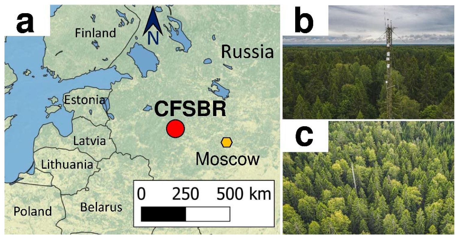
2.1. Study Site

This experimental study was performed in an old nemorose spruce forest, which is a widespread forest type in European southern taiga [46,47]. The study site is located in the southwest part of Valday Hills (56.4615° N, 32.9221° E, 265 m a.s.l.) in the core of the Central-Forest state biosphere reserve (CFSBR) in Tver region of Russia (Figure 1).
This region has a humid continental climate (Dfb type according to the Köppen–Geiger climate classification) [48] with cool winters and warm summers. The mean annual air temperature measured at meteostation (see Section 2.5) “Toropets” (56.48° N, 31.63° E, 187 m a.s.l.) in the 1991–2020 period was 5.7 °C (−5.9 °C in January and 18.2 in July °C). The growing season lasts, on average, 182 days (12 April–11 October). The mean annual precipitation according to the observations at meteorological station “Lesnoy Zapovednik” (56.50° N, 32.83° E, 240 m a.s.l.) in the same period was 778 mm. The snow cover forms in mid-November and melts in early April [49]. Precipitation is usually uniformly distributed over the year, with the maximum occurring in summer. Due to the positive moisture balance (precipitation exceeds potential evapotranspiration) and weak drainage of the glacial clay soils, the region is experiencing paludification processes [46,50].
According to the meteorological observations at the meteostations nearest to the CFSBR, “Toropets” and “Lesnoy Zapovednik”, positive air temperature (+0.73 °C per 10 years) and precipitation (+3.6 mm∙month−1 per 10 years) trends were detected in the study area during the 1991–2020 period; moreover, the growing season length is mostly increasing due to the shifting of the start of the growing season in spring to earlier dates [51].
The nemorose spruce forest (FLUXNET ID: Ru-Fy2) is located on a flat (<1°) well-drained slope with sod-pale podsolic soils Kurbatova et al. [43]. Tree vegetation includes Norway spruce (Picea abies), 53%; Norway maple (Acer platanoides), 18%; Scotch elm (Ulmus glabra), 6.4%; Eurasian aspen (Populus tremula), 6%; and white birch (Betula pubescens), 5%. Herbaceous vegetation is dominated by male-fern (Dryopteris filix-mas) and wood-sour (Oxalis acetosella) [32]. Tree vegetation ages up to 200 years and forms a closed canopy with heights up to 30–35 m and a leaf area index (LAI) of about 6.5 [52]. The soil C and N contents are estimated to be 68,000 kg∙ha−1 and 27–58 kg∙ha−1, respectively [53].

2.2. Flux Measurements

Ecosystem CO2 fluxes and additional environmental variables were obtained using eddy covariance and meteorological observations taken in the 2015–2020 period. The instruments used for flux measurements were mounted on the top of a 42 m tower. Eddy covariance system included a 3D sonic anemometer WindMaster Pro (Gill Instruments, Lymington, UK) and enclosed infrared CO2/H2O gas analyzer LI-7200 A (LI-COR Inc., Lincoln, NE, USA). Global radiation was measured by a 4-component radiometer CNR4 (Kipp & Zonen B.V., Delft, The Netherlands) at the height of 41 m. Additionally, the humidity and temperature probe HMP155 (Vaisala Inc., Vantaa, Finland) was mounted at the same height to obtain air temperature and humidity data. Precipitation measurements were carried out using two TR-525M (Texas Electronics Inc., Dallas, TX, USA) rain gauges installed at heights of 2 m and 30 m, respectively. The soil temperature and water content (SWC) were measured using 3 Stevens Hydroprobe II (Stevens Water monitoring Systems Inc., Portland, OR, USA) reflectometers at a depth of 5 cm. Flux data were stored on a flash drive using an LI-7550 (LI-COR Inc., USA) data logger every 0.1 s, while the meteorological data were collected by the LI-COR Biomet system 103 (LI-COR Inc., USA) every 1 min, respectively. The time in Moscow (UTC+3) was used for the data storage.

2.3. Data Processing and Statistical Analysis

Ecosystem CO2 fluxes were calculated for 30 min intervals using the Eddy Pro software (LI-COR Inc., USA). All necessary corrections and statistical tests were implemented under this processing. Footprint parameters were estimated using the model of Kljun et al. [54]. Quality flags were assigned to the calculated fluxes using the 0-2 flag policy according to Mauder and Foken [55]. All fluxes with flag 2 were excluded from the analysis following the recommendations from the data quality assessment [56]. Additionally, the 30 min flux values with flags 0 and 1 containing the spikes collected under rain and dew events and low turbulence were also filtered out. Storage terms calculated using the “one-point” approach following Greco and Baldocchi [57] were added to the flux values. The “one-point” approach allows one to calculate storage terms using CO2 concentration measurements at the top of the tower when the profile measurements are not available. NEE data were u*-filtered, gap-filled, and partitioned into TER and GPP using the REddyProc package [58]. The u* thresholds varied between 0.29 and 0.52 m∙s−1 in the period.
Uncertainty in the NEE, TER, and GPP associated with the random error in the flux measurements fluxes and data post-processing were calculated using the REddyProc package [58] as the standard deviation (SD) of the fluxes. The annual and seasonal random uncertainty aggregation for CO2 fluxes was calculated considering the autocorrelation between the residuals using the empirical autocorrelation function [59].
Since the daily TER, GPP, and NEE values did not show a normal distribution (Shapiro–Wilk’s test, p < 0.05), the statistical significance of the interannual differences in CO2 fluxes was estimated using the Mann–Whitney U-test (M-W U-test) and Kruskal–Wallis ANOVA (K-W test) with Dunn’s post hoc test. The differences were considered to be statistically significant under the p-value <0.05.

2.4. Estimation of the Dependence of TER and GPP to Environmental Variables

As the TER variations were mainly controlled by the soil and air temperatures and GPP generally follows the Rg variability, we analyzed the temperature sensitivity of the TER and light–response curves of GPP. The sensitivity of the night-time TER (µmol∙m−2∙s−1) to air and soil temperatures was estimated using the Q10 model following [60]:
Q 10 = exp 10   ·   α
where α is an empirical parameter of the following equation:
Ln TER = α   ·   T + γ
where T is soil or air temperature (°C) and γ is an empirical parameter of the equation. Equation (2) was also used to derive the R10 coefficient as a night-time respiration rate under a 10 °C soil or air temperature.
To describe the dependence of GPP on Rg (W∙m−2), a Michaelis–Menten hyperbolic light–response curve was used in the following form:
GPP = ε   ·   β   ·   Rg ε   ·   Rg + β
where ε and β are the empirical parameters of the curve: the canopy light utilization parameter (µmol∙J−1) and the maximum CO2 uptake at light saturation (µmol∙m−2∙s−1), respectively [61]. Only the original 30 min NEE data were used to obtain TER and GPP for these analyses.

2.5. Additional Data

Air temperature and precipitation data from two meteorological stations situated close to the study sites were used for the analysis of the weather conditions in the period 2015–2020. Precipitation and snow cover data were obtained from the area nearest to the site’s meteorological station “Lesnoy Zapovednik”, which was located 4.5 km from the flux station. Due to lack of available night-time observations at “Lesnoy Zapovednik”, air temperature data from the “Toropets” meteostation located 40 km west of the reserve were taken from the RIHMI-WDC database (http://aisori-m.meteo.ru; access date: 20 May 2022).

3. Results

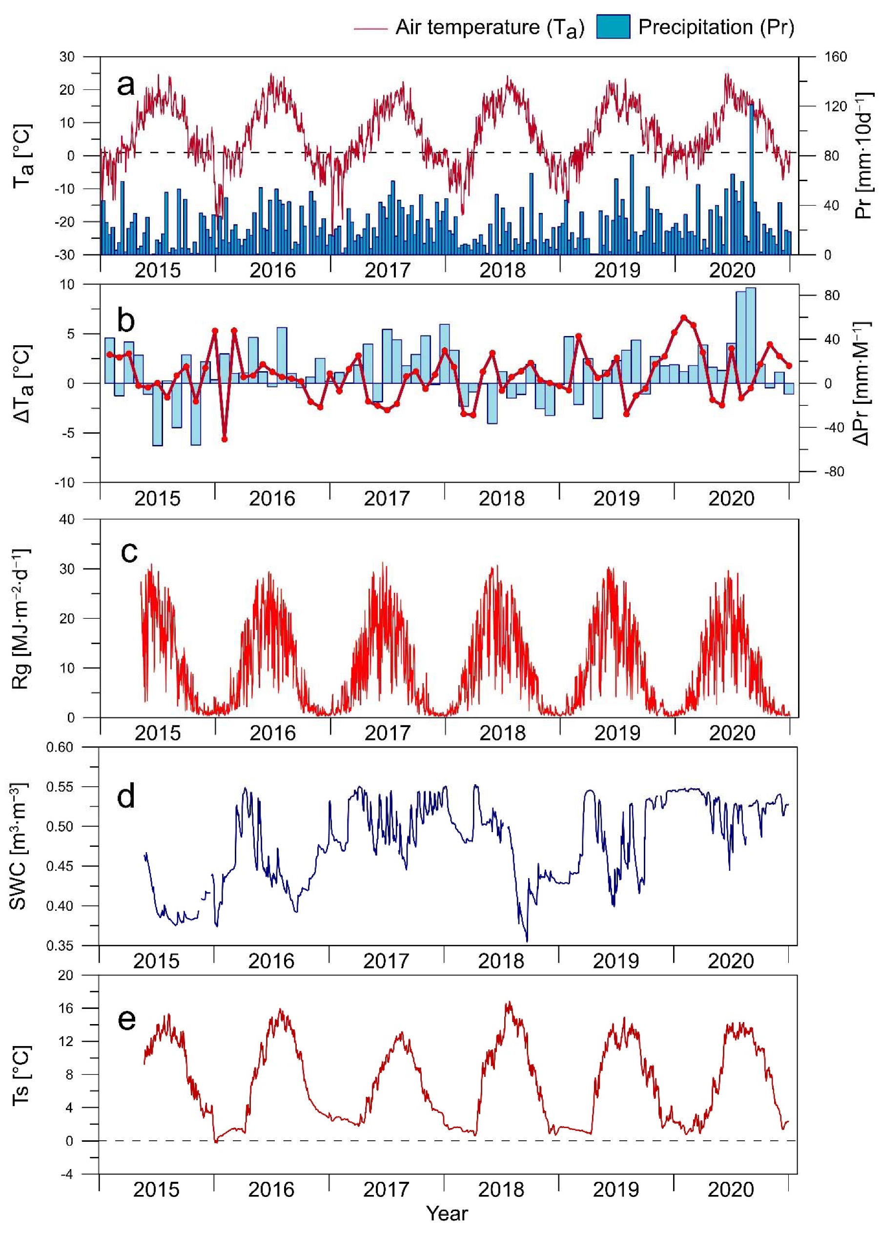
3.1. Environmental Conditions
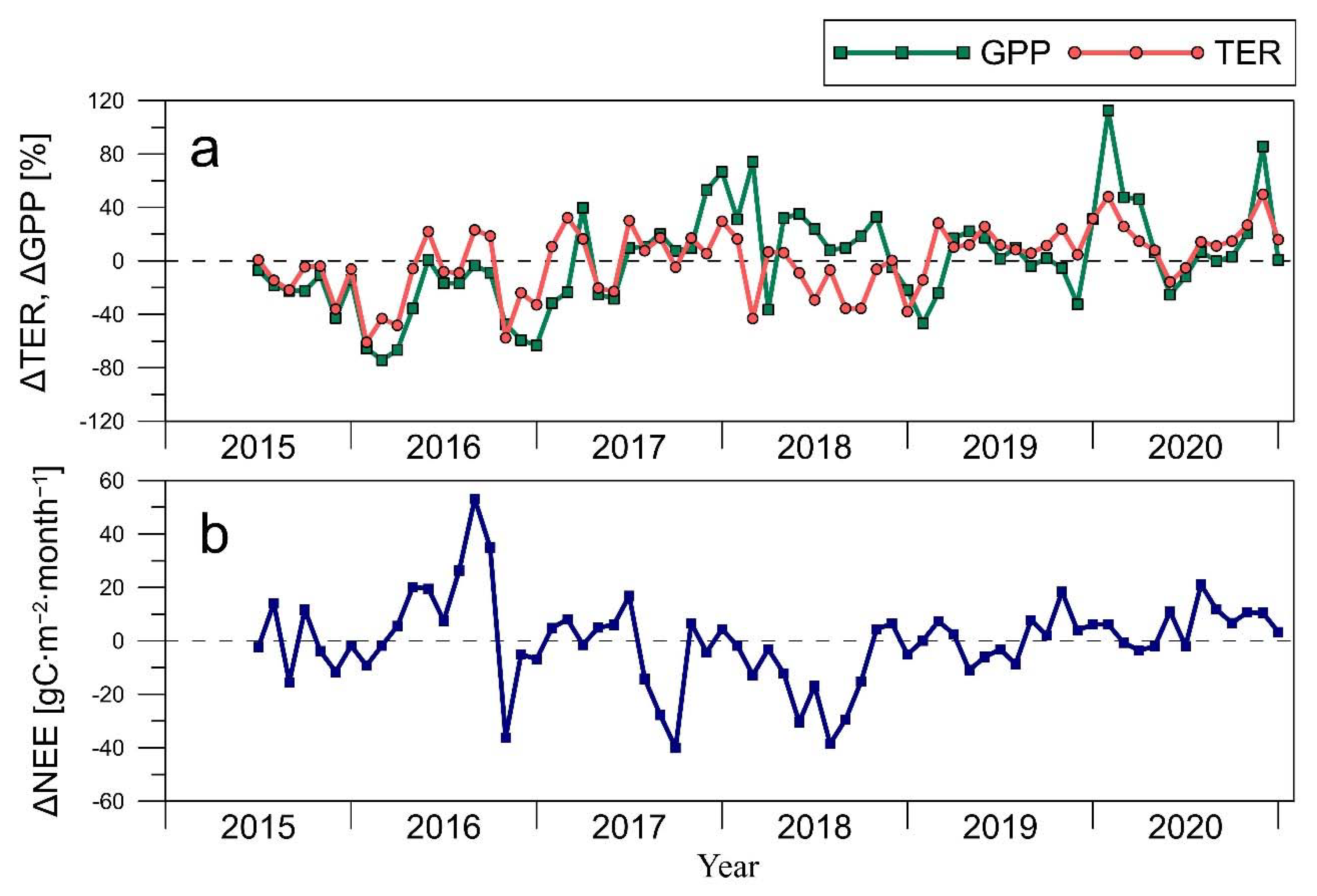
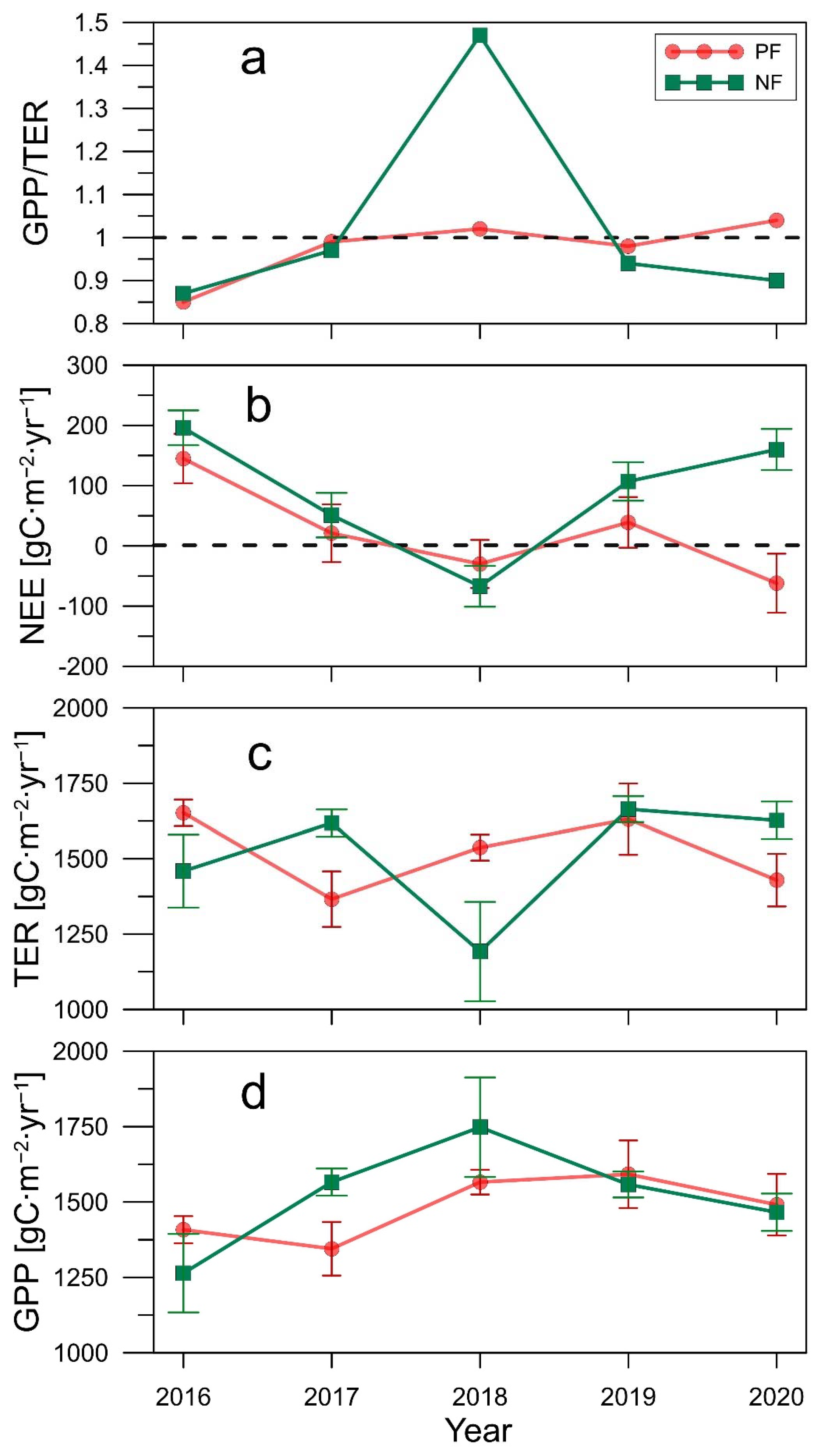
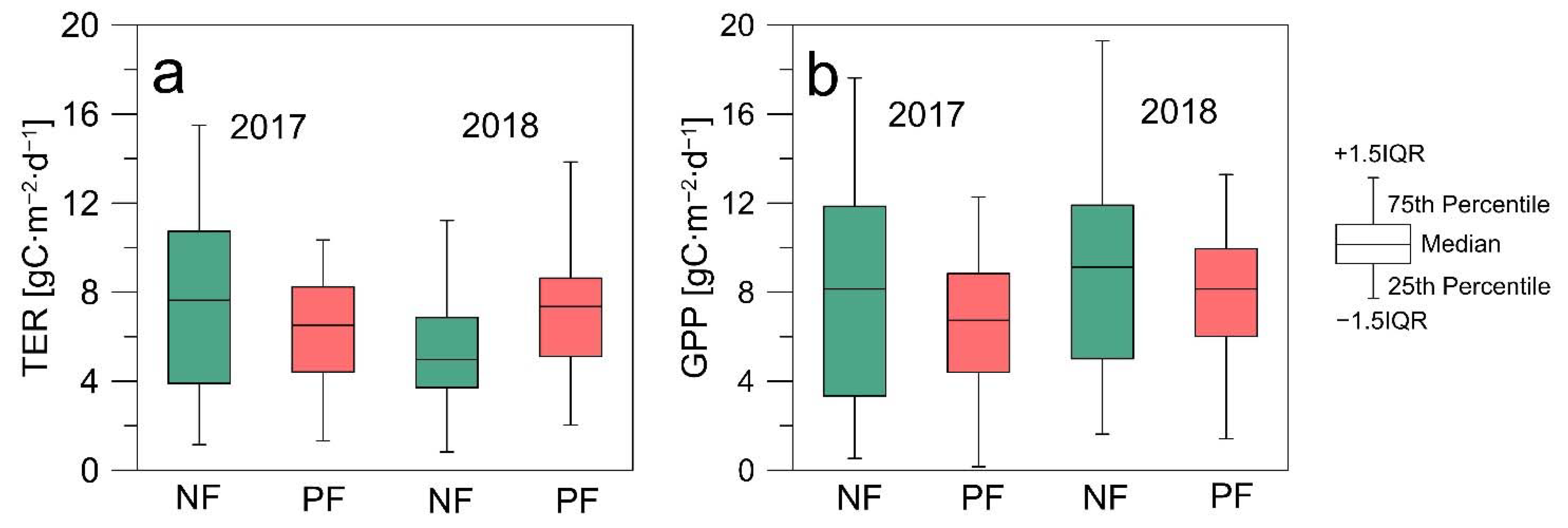
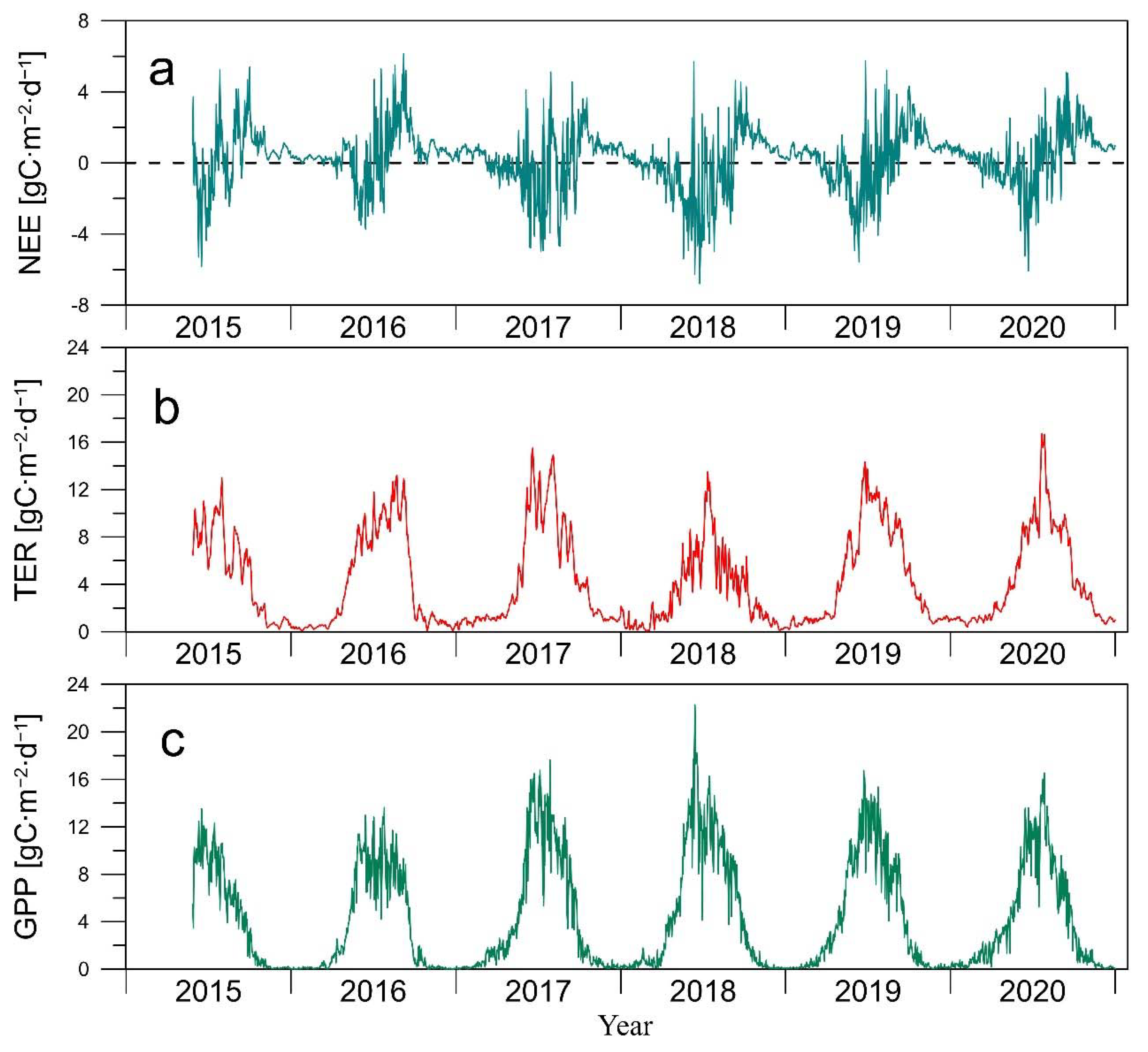
According to the observations made at meteorological station “Toropets”, five of six years of the 2015–2020 period were warmer in relation to the long-term means (Table 1); moreover, no years with a negative annual temperature anomaly were observed in the period [51]. The coolest year was 2017, when the mean annual air temperature was equal to the long-term annual mean, and the warmest year was 2020, when the mean annual temperature anomaly reached 1.9 °C. According to the observations made at the meteorological station “Lesnoy Zapovednik”, the annual precipitation in 2015 and 2018 was lower than the mean long-term annual sum. Other years of this period were relatively wet, with annual precipitation exceeding the long-term means. The wettest year was 2020, when the annual precipitation exceeded the long-term mean value of 22%.
Unlike the mean annual air temperature, the mean air temperature calculated for the long-term growing season (LTGS) period (12 April–11 October) was lower than its mean 30-year value in 2015, 2017, and 2019 and higher than it in other years. The coldest growing season was 2017, and the warmest one was 2018. Precipitation sums were lower than the LTGS mean value in 2015 and 2018 and higher in other years of the period. The driest growing season was 2015, and the wettest one was 2020. The mean winter (1 November–31 March) air temperature was lower than the long-term mean values only in the winter of 2017/2018 (Table 2). Other winters were relatively warm, and a particularly high mean winter temperature was observed in the winter of 2019/2020. The winter air temperature anomalies in the 2015–2020 period were primarily positive, while negative temperature anomalies were generally detected in spring and summer (Figure 2). Precipitation anomalies were differently distributed across the years of measurements. The most significant precipitation anomalies (both positive and negative) were observed in summers.
According to the observations made at meteorological station “Lesnoy Zapovednik” in the selected years, the surface was covered by snow from November to April with a maximum snow depth of about 40 cm. Under the exceptionally warm conditions that occurred in winter 2019/2020, snow cover was detected only in January and February 2020, with a maximum snow depth of 10 cm [51].
The minimal values of annual global radiation (Table 1) were observed in the wettest and coolest year of the period, 2017. The maximal sum of Rg was detected in the year with relatively dry and warm weather conditions in the growing season, 2018. The daily soil temperature variations followed the air temperature variations, reaching 0 °C in winter and 17 °C in summer. Unlike the air temperature, the soil temperature was positive in the winters, and its mean annual value was less variable across the years. The soil water content (SWC) at the site varied between 0.35 and 55 m3∙m−3. The maximal values were observed in the springs, shortly after the snowmelts and after the periods of heavy rain occurring in the summer and autumn. The seasonal course of the SWC had a pronounced pattern: after the snow melted, it tended to decrease, and the minimal values were generally observed in August and September before slightly increasing until spring. The minimal value of the SWC obtained for the study period was observed in the summer of 2018, which was the driest year of the period. In the relatively wet growing seasons (2017 and 2020), the summer SWC was usually higher than 45 m3∙m−3. The mean annual SWC was correlated with the annual precipitation measured at the meteorological station “Lesnoy Zapovednik” (Table 1).

3.2. CO2 Fluxes

Eddy covariance flux measurements conducted in the 2015–2020 period showed that the nemorose spruce forest was a CO2 source or sink, depending on the year of the measurements. The annual sums of NEE were primarily positive, with the maximum occurring in 2016 (Table 3). The nemorose forest was a source of atmospheric CO2 in all the years of measurements, excepting 2018, when under the relatively high temperature and global radiation as well as low precipitation, the GPP reached its maximal values, and the TER was minimal. The mean daily GPP/TER was significantly lower in 2016 and higher in 2018 than in the other years (K-W test, H = 119.040, n = 1827, p < 0.001; Dunn’s post hoc test p < 0.044 for 2016 and p < 0.001 for 2018). In 2018, the mean annual GPP/TER ratio reached 1.47, while it was between 0.87 and 0.97 in the other years.
The annual sums of NEE, TER, and GPP were mostly determined by the CO2 fluxes seen in the growing season. Thus, the growing season sums calculated for the mean long-term growing season period (12 April–11 October) determined 85–91% of the annual TER and 93–97% of the annual GPP. Unlike the annual sums in the growing season, the nemorose spruce forest was found to primarily be a sink of atmospheric CO2. The growing season NEE was positive (TER > GPP) in 2016 and 2020 and negative in 2017–2019 (GPP > TER). However, considering the aggregated uncertainty of the growing season sums of the CO2 fluxes, it is difficult to identify the status of the nemorose spruce forest as a CO2 sink or source in the growing seasons of 2017, 2019, and 2020.
The strongest CO2 source was detected in the growing season of 2016 (GPP/TER = 0.91), and the strongest sink was detected in the growing season of 2018 (GPP/TER = 1.63). The negative (2016) and positive (2018) anomalies in the mean daily GPP/TER in the growing seasons were significant (K-W test, H = 202.314, n = 915, p < 0.001; Dunn’s post hoc test p < 0.003). Increased CO2 uptake in the growing season of 2018 was determined by the decreased TER and increased GPP.
In all winters (1 November-31 December) of the period, the nemorose forest acted as a slight CO2 source (Table 4). Under the strong positive temperature anomaly and sparse snow cover observed in the winter of 2019/2020 increases in both daily TER and GPP were detected (K-W test, H = 141.092, n = 757, p < 0.001 for TER and H = 116.257, n= 757, p < 0.001 for GPP; Dunn’s post hoc test p < 0.001). Despite the mean GPP/TER ratio in the winter of 2019/2020 being the highest among the winters of the period and significantly higher than the mean GPP/TER values for the other years (M-U test U = 40,617, p = 0.026), the winter NEE was also higher (M-U test U = 37685, p < 0.001) and reached the maximal value.
The seasonal variability of the daily NEE, TER, and GPP in the study period had the following pattern: In winter, the forest was a slight source of atmospheric CO2, with small NEE (0–2 gC∙m−2∙d−1), TER, and GPP values (Figure 3). In winter, the NEE slowly decreased between November and March due to the decrease in TER and slight growth of the GPP from February. In the April–July period, the forest generally acted as a CO2 sink, as the GPP increased faster than the TER could reach the maximum CO2 uptake rates in June (up to NEE = 7 gC∙m−2∙d−1 and GPP = 22 gC∙m−2∙d−1). From August to mid-November, the forest was usually a strong CO2 source, as the TER decreased slower than the GPP (NEE reached 6 gC∙m−2∙d−1).
The interannual variations in the environmental conditions led to the changes in the typical TER, GPP, and, consequently, NEE courses. To show the relative differences in CO2 fluxes within the period of study, we calculated the anomalies in the monthly TER and GPP as the difference between the sum of GPP or TER for the month and its mean value in the 2015–2020 period expressed in % relative to the mean sum of the TER or GPP for each month, respectively (Figure 4), as well as absolute anomalies of NEE. The relative anomalies of TER and GPP, as well as the NEE anomalies, were positive or negative depending on the weather conditions and varied over the months and years. For example, in the growing season of 2017, under the low Rg, air temperature, and high precipitation, relatively low TER and GPP values with relatively high NEE values were observed, but in summer, conversely, the TER and GPP values were relatively high with relatively low NEE values. In the dry, warm, and sunny growing season of 2018, relatively low TER values and high GPP values were detected. This provided the lowest NEE values seen out of the entire period of measurements. Under the warm and wet conditions observed in the growing season of 2020, the GPP and TER anomalies were found to be positive, with the NEE shifting to higher values.
Whereas the changes in daily flux values that occurred between the selected years were maximal in the growing seasons, the differences in the relative TER and GPP anomalies were more pronounced in the winters. According to the meteorological observations, positive temperature anomalies were detected every winter of the period (Figure 2). Cooler winters were characterized by negative GPP and TER anomalies with small changes in NEE. By contrast, the exceptionally warm weather conditions seen in winter 2019/2020 led to the positive anomalies seen in GPP and TER. The NEE anomaly was positive from November 2019 to January 2020, but in March 2020, the NEE anomaly was negative.
Hereby, the warm and sunny growing season of 2018 with the negative precipitation anomaly provided the most significant changes in CO2 exchange seen among study years, with the nemorose spruce forest switching from a CO2 source to a CO2 sink, while the strong positive temperature anomaly seen in the winter of 2019/2020 did not change the annual NEE substantially.

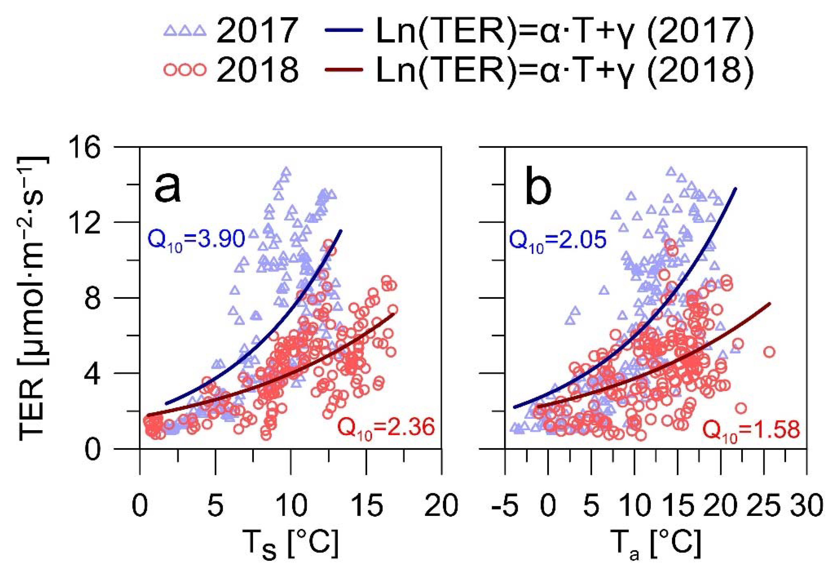
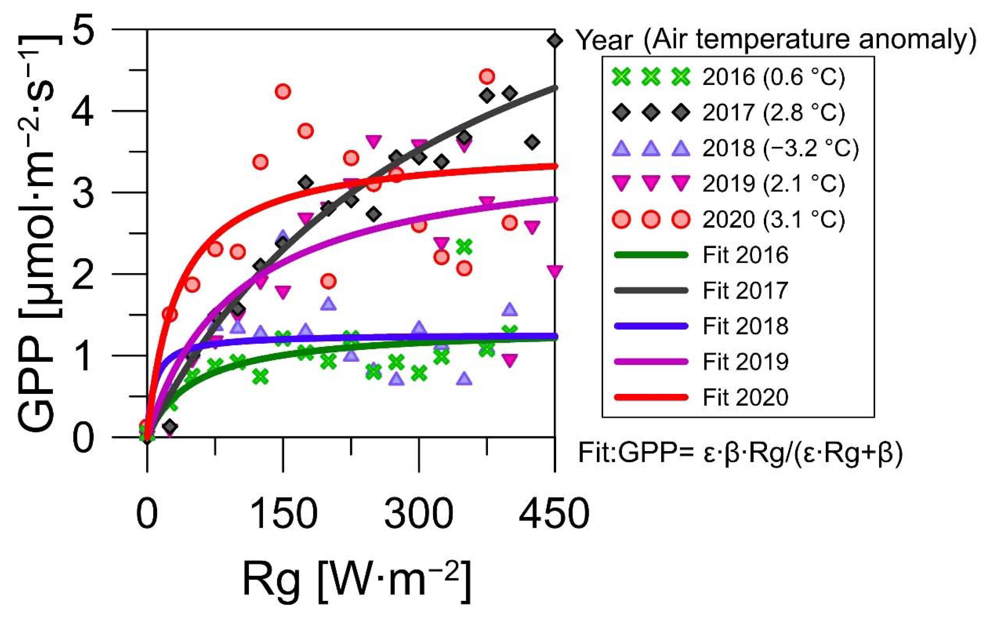
3.3. Environmental Factors of the CO2 Fluxes

The GPP and TER variations seen during the study period were determined by the changes in environmental conditions. TER was controlled by the air and soil temperatures, but the sensitivity of TER to Ta and Ts had its own interannual variability. To demonstrate the difference in the temperature sensitivity parameters of TER over the years of measurements, we compared the dependence of the mean night-time TER obtained in the period from 1 May to 31 October on the Ta and Ts between two contrasting growing seasons: a relatively wet and cool 2017 and a relatively dry and warm 2018 (Figure 5, Table 5). In spite of the lower temperatures observed in 2017 (relative to 2018), TER changed within a broader range. The approximation of the dependence with the Q10 model (Equation 2) showed that the TER in a relatively wet year was more sensitive to temperature variations. Due to the negative correlations seen between the temperatures and SWC, it is challenging to attribute the unexplained variability of TER to SWC variations at daily and seasonal scales.
GPP was mainly controlled by Rg, but the light–response curve parameters were found to be sensitive to air temperature variations. The positive temperature anomalies that occurred in winter and early spring led to the changes seen in GPP sensitivity to Rg and increased the GPP at the site. To show how temperature anomalies influence the relationship between GPP and Rg in early spring, we compared the hyperbolic light–response curves (Equation 3) of GPP obtained in March 2016 (−0.6 °C), when the air temperature was close to the long-term mean; March 2018 ((−4.5 °C), under the influence of the negative temperature anomaly; March 2017 (1.6 °C), 2019 (0.8 °C) and 2020 (1.9 °C), under the influence of the positive temperature anomaly (Figure 6, Table 6). According to the meteorological data taken from the “Toropets” meteostation, the long-term mean air temperature (1991–2020) in March was (−1.3 °C. The GPP rates obtained in the anomalously warm March of 2017, 2019, and 2020 were higher than those obtained in March 2016 and 2018 under similar Rg values. Unlike the positive air temperature anomalies observed in 2017, 2019, and 2020, the negative one saw in 2018 did not significantly change the shape of the light–response curve in relation to that seen in March 2016. The positive temperature anomaly increased the β coefficient of the hyperbolic function, which refers to the saturation point of the curve. As GPP was not limited by water availability, the air temperature is a key factor controlling the GPP and CO2 balance of the nemorose spruce forest in early spring.

4. Discussion

4.1. Ecosystem–Atmosphere CO2 Exchange in the Spruce Forests

Eddy covariance flux measurements in the 2015–2020 period showed that a southern taiga nemorose spruce forest was a CO2 sink or source for the atmosphere depending on the GPP/TER ratio, which was controlled by the environmental conditions of the particular year. Since the estimated uncertainty of the flux measurements was comparable to the annual NEE value, it is likely that the forest was generally a slight annual CO2 source and was almost CO2 neutral in the growing seasons. The annual NEE in the nemorose spruce forest changed between −67 ± 34 and 196 ± 29 gC∙m−2. The annual NEE sums reported in this study correspond to the estimates obtained from old boreal spruce forests located in the other geographical regions of North America and Europe–e.g., Ueyama et al. [10], Liu et al. [21], and Lindroth et al. [62]—which were sources of the atmospheric carbon dioxide or CO2-neutral. However, many other mixed spruce stands have significant annual CO2 uptake rates. For example, an old spruce forest near Valday Lake (Novgorodskaya oblast, Russia), located 170 km north of the study site, was found to be a CO2 sink, with an annual NEE ranging between (−300 and −95 gC∙m−2 [45] in the 2010–2018 period.
Mid-aged stands usually have higher CO2 uptake rates [9]. Flux measurements taken from a mid-aged hemiboreal forest in Estonia in 2015 showed an annual NEE of −586 ± 45 gC∙m−2 [63]. Grünwald and Bernhofer [64] reported an NEE in an old mixed spruce forest in Tharandt (Germany) of between −395 and −698 gC∙m−2. The annual NEE obtained by Jensen et al. [65] in a spruce forest with trees of different ages in Denmark during 6 years of measurements was between −553 and −937 gC∙m−2. Twenty years of flux measurements taken from a mixed spruce forest in Ardennes (Belgium) showed an NEE of about −411 gC∙m−2 per year [36].
The interannual variability of NEE was dependent on the GPP/TER ratio. The flux measurements taken from an old southern taiga nemorose spruce forest in the 2015–2020 period showed that the annual GPP/TER ratio at the study site varied between 0.87 and 1.47 and showed increased values in 2018 due to the relatively dry, sunny, and warm growing season conditions detected. The GPP/TER ratio obtained by Krasnova et al. [63] in a mixed spruce stand in Estonia was about 1.84. Lindroth et al. [62] reported a GPP/TER ratio of a mixed spruce forest in Sweden of about 0.75. The GPP/TER ratio obtained by Jensen et al. [65] in a spruce forest in Denmark was 1.49–1.88. Amiro et al. [66] reported that different post-harvest and post-fire 20–100-year-old stands in North America have a GPP/TER ratio of between 0.8 and 1.8. Therefore, the GPP/TER ratio obtained in this study is within the range of that of other boreal and temperate forests. The lower GPP/TER ratio of the nemorose spruce forest in Valdai hills (this study) and the mixed spruce forest from Sweden [62] in comparison with other mixed forests located in Estonia [63], Germany [64], and Denmark [65] can be explained by the high TER rates, as the GPP values in the all of the selected studies had similar magnitudes. TER in the studies conducted by Grünwald and Bernhofer [64], Krasnova et al. [63], and Jensen et al. [65] was about 700−1400 gC∙m−2, and GPP was about 1300−2000 gC∙m−2.

4.2. Implications of the Heatwaves for the CO2 Exchange of the Spruce Forests

The most substantial increase in CO2 uptake at the study site in the 2015–2020 period was detected in 2018 when a significant part of Europe experienced a heatwave. Several modeling experiments and in situ observations showed a decrease in the CO2 uptake in summer 2018 for many ecosystem types, including forests, peatlands, grasslands, and agricultural lands, which were primarily associated with decreased GPP limited by high VPD and soil moisture stress values [25,30,32,67]. For example, the comparison of the flux data obtained in four ecosystems in Estonia—mixed spruce forest, deciduous forest, coniferous (spruce, pine) forest, and clear cut in 2017 and 2018 [68]—showed that the heatwave of 2018 decreased the net CO2 uptake of the ecosystems. This was caused by the decrease in GPP due to water stress, which canceled out the effect of the decrease in TER and also increased the annual CO2 released by the ecosystems. The difference in the ecosystems’ response to the heatwave is possibly related to the soil water availability and VPD dynamics at the sites. SWC in a mixed forest in Estonia in the summer of 2018 dropped to the values of less than 0.10 m3∙ m−3 [68], while at the study site in the Valdai Hills, it was higher than 0.35 m3∙ m−3. The VPD at the study site in the summer of 2018 was lower than reported by Krasnova et al. [68]. On some days, the midday VPD of the nemorose spruce forest in the Valdai Hills (this study) exceeded 20 hPa, but the mean summer value at the site was 5.3 ± 5.1 hPa (±SD). A positive GPP anomaly in summer 2018 detected at the study site corresponded to the results of the modeling study conducted by Smith et al. [25], who showed a slight positive GPP anomaly for the region during the heatwave of 2018.
The important feature of the CO2 flux dynamics in many boreal forests is that the maximum CO2 uptake usually is observed in spring due to the fast increase in GPP at the beginning of the growing season, while the maximal TER lags behind, occurring in mid-summer. Thus, a high GPP rate in the growing season of 2018 at the nemorose spruce forest was provided by the significant Rg due to the high frequency of clear sky days and the air temperatures being favorable for photosynthesis. Yet, it is possible that the thawing water supply provided enough moisture to the soil in spring when the maximum CO2 uptake was observed in spite of the negative precipitation anomalies. Otherwise, the decrease in the SWC of the upper soil layer provided a decreased TER in summer, which corresponded to previous in situ estimates of TER and its components at the paludified spruce forest located 1.5 km from the study site during the 2002–2012 period and covering a drought that occurred in 2010 in West Russia [69]. However, unlike in 2010, the summer precipitation that occurred in 2018 was enough to prevent the deep soil layers from experiencing drought. Additionally, it is possible that the winter precipitation and thawing water supply are important factors that can affect the annual and growing season NEE of the nemorose spruce forest as well as other boreal forest ecosystems [18,70,71] and potentially mitigate the effect of the decreased precipitation occurring in spring and summer.
Unlike the relatively warm, sunny, and dry growing season of 2018, the anomalously warm winter with a thin snow cover of 2019/2020 led to the substantial positive GPP anomalies seen in late winter and early spring but did not alter the annual sums of NEE too significantly. As the winter and early spring GPP of forests located at high latitudes are limited by low temperatures and radiation, the temperature anomaly may have led to the early beginning of the CO2 uptake [21,72]. The modeling study conducted by Kwon et al. [71] showed similar results for the air temperature anomalies seen in the winter and spring of 2019/2020 in Siberia, when the forest ecosystems demonstrated an increased spring CO2 uptake but no increase in the annual uptake due to the substantial CO2 loss in summer. If a warm spring is followed by a negative precipitation anomaly in summer, the water stress may lead to a decreased annual CO2 uptake in forest ecosystems [27,73]; moreover, increased water consumption due to the early beginning of the growing season in spring may alleviate this effect due to the increased evapotranspiration demands [21,24].

4.3. Implications of the Local Soil Moisture Regimes for the CO2 Exchange of Spruce Forests

The hydrological regime of the site may be the key factor that determines the response of a forest ecosystem to climate extremes and anomalies. The results obtained from the flux measurements performed in the southern taiga nemorose spruce forest were different from the results obtained from an old paludified spruce forest (Ru-Fyo FLUXNET ID) located 1.5 km from the study site [51]. While the ecosystem CO2 uptake in the nemorose spruce forest substantially increased in 2018, the annual GPP/TER ratio in the paludified spruce forest was less sensitive to the warm, dry, and sunny environmental conditions (Figure 7). Conversely, the CO2 uptake of the paludified forest in 2020 increased significantly due to the anomalously warm conditions observed in winter and at the beginning of spring. The growing season TER at the paludified forest in 2020 decreased due to the high water levels seen in summer caused by a positive precipitation anomaly. In the nemorose forest, the early start of the CO2 uptake, as well as the TER dynamics, did not lead to an increase in the annual GPP/TER ratio. The annual sums of the CO2 fluxes seen at the sites in the 2016–2020 period had a similar order of magnitude: NEE in the paludified forest varied between −95 ± 12 and 145 ± 41 gC∙m−2, TER varied between 1366 ± 92 and 1652 ± 44 gC∙m−2, and GPP varied between 1408 ± 45 and 1592 ± 112 gC∙m−2, respectively [51]. However, the daily CO2 fluxes in the nemorose spruce forest varied within a wider range (Figure 8). This is likely connected with the high ground water level seen in the paludified spruce forest (close to the surface), which on the one hand, will mitigate the effect of the precipitation variability and preserve a consistent water supply in the soil, and on the other hand, create wet anoxic conditions and inhibit the respiration as well as productivity of spruce [11,74].
The comparison of the CO2 fluxes observed in the two different southern taiga spruce forests in the growing seasons with the negative temperature and positive precipitation anomaly that occurred in 2017 and with the positive temperature and negative precipitation anomaly that occurred in 2018 showed that the TER at the nemorose spruce forest was higher in the cool and wet year of 2017 (M-W U test, U = 12,275, Z = 4.42, p < 0.001), while the TER in the paludified forest was higher in 2018 (M-W U test, U = 13,955, Z = (−2.76, p = 0.006). The previous study conducted by Kurbatova et al. [69] reported that soil respiration is the major component of TER in paludified spruce forests. Additionally, it is likely that the soil respiration and TER of the nemorose spruce forest in summer are limited by the water availability in the soil. In contrast, the soil respiration and consequently TER of the paludified forest is limited by soil aeration, which is generally low due to the high ground water levels. This may explain the different responses of the TER to the dry conditions experienced in summer 2018. However, in the case of a severe drought, a decreased TER in a paludified forest due to the water stress is very possible. Such an effect was observed in the paludified spruce forest during the extreme drought event that occurred in 2010 [69].
The GPP at both of the sites was higher in 2018 than in 2017 (in the nemorose spruce forest, M-W U test, U = 14,534, Z = −2.18, p = 0.029; in the paludified spruce forest, M-W U test, U = 12,400, Z = (−4.29, p < 0.001). Both ecosystems showed increased primary production in the growing season in response to the high radiation and air temperatures, but the effect was less pronounced for the paludified spruce forest due to its relatively low productivity [51].
The GPP/TER ratio of the nemorose spruce forest was less sensitive to the air temperature anomaly that occurred in the winter of 2019/2020 than in the paludified spruce forest (Figure 9). We suppose that this difference may be related to the greater portion of spruce in the tree vegetation composition in the paludified forest or the higher fraction of heterotrophic respiration in TER in the nemorose spruce forest. Additional observational data considering the components of TER in winter in the two forests are needed to test these hypotheses.
This study experimentally demonstrated that local hydrology and soil moisture regimes are important environmental factors that determine the differences in the response reactions of the ecosystem CO2 exchange in forest ecosystems to climate extremes and anomalies and should be considered in future projections of forest atmosphere exchange [26,28]. Soil moisture controls water and nutrient availability to plants as well as influencing the vegetation composition, structure, and productivity of forest ecosystems, determining the ecosystem–atmosphere feedback. Depending on the severity and duration of extreme events, the reaction of NEE may vary [27]. Considering the current climate trend seen in the Valday Hills—an increase in the winter temperatures and a shift in the start of the growing season to an earlier date [75]—we expect to see an increase in the CO2 uptake of nemorose and paludified spruce forests in the winter to spring transition in the future. The response of an ecosystem to heatwaves occurring in the growing season can differ depending on the moisture regime at the particular site: if GPP is not limited by the available ground water or high VPD, an increase in the CO2 uptake of the forest can be expected [27], but the loss of CO2 at sites which usually have a high water level can cancel out the effect of the increased GPP and lead to smaller changes in NEE than would be seen at well-drained sites. A high frequency of summer heatwaves or lack of thaw water can also lead to the accumulation of water stress and negatively influence CO2 uptake [28]. In the case of a higher frequency of severe and long droughts, as observed in 2010 and predicted for the region in the future [6], a decrease in GPP, as well as TER in paludified and well-drained spruce forests, is possible, as well as a decrease in CO2 uptake.

5. Conclusions

Eddy covariance flux measurements taken in the 2015–2020 period show that the southern taiga old nemorose spruce forest acts as an atmospheric CO2 source or sink in both the annual and growing season time scales depending on the environmental conditions of the particular year. The changes in the NEE of the forest are dependent on the GPP/TER ratio variability. The anomalously dry, warm, and sunny conditions observed in the growing season (2018) led to an increase in CO2 uptake from the atmosphere due to the increased GPP and decreased TER observed at the site. Anomalously warm winter conditions provided an early CO2 uptake in spring in the nemorose spruce forest; however, it did not increase the annual GPP/TER ratio. The TER in the cool and wet growing season (2017) was more sensitive to the temperature variations than in the dry and warm (2018). The comparison of the flux data obtained from the nemorose spruce forest on well-drained mineral soils with the estimates obtained from the paludified spruce forest [51] located within the same landscape showed that the NEE, GPP, TER, and GPP/TER ratio of the ecosystems differently responds to the changes in the environmental conditions. The opposite dynamics of TER at the sites between the cool and wet (2017) and the warm and dry (2018) growing seasons were detected. Therefore, the difference in the local soil moisture regimes of the southern taiga spruce forests may lead to alternative responses of the CO2 ecosystem–atmosphere exchange to climate anomalies. Additional data containing long-term flux measurements from southern taiga forest ecosystems are essential to test this hypothesis and to estimate the range of potential variability in the ecosystem–atmosphere CO2 exchange due to the local differences in the soil moisture regimes.

Author Contributions

Writing—original draft preparation, V.M.; data curation, project administration, A.V.; visualization I.Y.; supervision, J.K. All authors have read and agreed to the published version of the manuscript.

Funding

This study was supported by the grant of the Russian Science Foundation (21-14-00209).

Institutional Review Board Statement

Not applicable.

Informed Consent Statement

Not applicable.

Data Availability Statement

The meteorological and flux data used in the study are available upon request at European fluxes database cluster (http://www.europe-fluxdata.eu; access date: 20 May 2022).

Acknowledgments

We thank Dmitry Ivanov from A.N. Severtsov Institute of Ecology and Evolution of RAS (Moscow, Russia) for the photos of the flux towers in the nemorose spruce forest and in the paludified spruce forest (Ru-Fy2 and Ru-Fyo FLUXNET stations).

Conflicts of Interest

The authors declare no conflict of interest.

References

  1. Tagesson, T.; Schurgers, G.; Horion, S.; Ciais, P.; Tian, F.; Brandt, M.; Ahlström, A.; Wigneron, J.-P.; Ardö, J.; Olin, S.; et al. Recent divergence in the contributions of tropical and boreal forests to the terrestrial carbon sink. Nat. Ecol. Evol. 2020, 4, 202–209. [Google Scholar] [CrossRef] [PubMed]
  2. Chapin, F.S.; Randerson, J.T.; McGuire, A.D.; Foley, J.A.; Field, C.B. Changing feedbacks in the climate–biosphere system. Front. Ecol. Environ. 2008, 6, 313–320. [Google Scholar] [CrossRef]
  3. Bonan, G.B. Forests and climate change: Forcings, feedbacks, and the climate benefits of forests. Science 2008, 320, 1444–1449. [Google Scholar] [CrossRef] [PubMed] [Green Version]
  4. Lal, R.; Smith, P.; Jungkunst, H.F.; Mitsch, W.J.; Lehmann, J.; Nair, P.R.; McBratney, A.B.; Carlos de Moraes Sá, J.; Schneider, J.; Zinn, Y.L.; et al. The carbon sequestration potential of terrestrial ecosystems. J. Soil Water Conserv. 2018, 73, 145A–152A. [Google Scholar] [CrossRef] [Green Version]
  5. Schewe, J.; Gosling, S.N.; Reyer, C.; Zhao, F.; Ciais, P.; Elliott, J.; Francois, L.; Huber, V.; Lotze, H.K.; Seneviratne, S.I.; et al. State-of-the-art global models underestimate impacts from climate extremes. Nat. Commun. 2019, 10, 1005. [Google Scholar] [CrossRef] [Green Version]
  6. IPCC. Climate Change 2021. The Physical Science Basis; Cambridge University Press: Cambridge, UK, 2021; in press. [Google Scholar]
  7. Woodwell, G.M.; Whittaker, R.H. Primary production in terrestrial ecosystems. Am. Zool. 1968, 8, 19–30. [Google Scholar] [CrossRef]
  8. Chapin, F.S.; Woodwell, G.M.; Randerson, J.T.; Lovett, G.M.; Rastetter, E.B.; Baldocchi, D.D.; Clark, D.A.; Harmon, M.E.; Schimel, D.S.; Valentini, R.; et al. Reconciling carbon-cycle concepts, terminology, and methods. Ecosystems 2006, 9, 1041–1050. [Google Scholar] [CrossRef] [Green Version]
  9. Coursolle, C.; Margolis, H.A.; Giasson, M.A.; Bernier, P.Y.; Amiro, B.D.; Arain, M.A.; Barr, A.G.; Black, T.A.; Goulden, M.L.; McCaughey, J.H.; et al. Influence of stand age on the magnitude and seasonality of carbon fluxes in Canadian forests. Agric. For. Meteorol. 2012, 165, 136–148. [Google Scholar] [CrossRef] [Green Version]
  10. Ueyama, M.; Iwata, H.; Harazono, Y. Autumn warming reduces the CO2 sink of a black spruce forest in interior Alaska based on a nine-year eddy covariance measurement. Glob. Chang. Biol. 2014, 20, 1161–1173. [Google Scholar] [CrossRef]
  11. Lafleur, B.; Fenton, N.J.; Bergeron, Y. Forecasting the development of boreal paludified forests in response to climate change: A case study using Ontario ecosite classification. For. Ecosyst. 2015, 2, 1–11. [Google Scholar] [CrossRef] [Green Version]
  12. Seidl, R.; Thom, D.; Kautz, M.; Martin-Benito, D.; Peltoniemi, M.; Vacchiano, G.; Wild, J.; Ascoli, D.; Petr, M.; Honkaniemi, J.; et al. Forest disturbances under climate change. Nat. Clim. Chang. 2017, 7, 395–402. [Google Scholar] [CrossRef] [PubMed] [Green Version]
  13. Zhao, B.; Donnelly, A.; Schwartz, M.D. Evaluating autumn phenology derived from field observations, satellite data, and carbon flux measurements in a northern mixed forest, USA. Int. J. Biometeorol. 2020, 64, 713–727. [Google Scholar] [CrossRef] [PubMed]
  14. Piao, S.; Friedlingstein, P.; Ciais, P.; Viovy, N.; Demarty, J. Growing season extension and its impact on terrestrial carbon cycle in the Northern Hemisphere over the past 2 decades. Glob. Biogeochem. Cycles 2007, 21, GB3018. [Google Scholar] [CrossRef]
  15. Thomas, R.T.; Prentice, I.C.; Graven, H.; Ciais, P.; Fisher, J.B.; Hayes, D.J.; Huang, M.; Huntzinger, D.N.; Ito, A.; Jain, A.; et al. Increased light-use efficiency in northern terrestrial ecosystems indicated by CO2 and greening observations. Geophys. Res. Lett. 2016, 43, 11–339. [Google Scholar] [CrossRef]
  16. Fu, Z.; Dong, J.; Zhou, Y.; Stoy, P.C.; Niu, S. Long term trend and interannual variability of land carbon uptake—The attribution and processes. Environ. Res. Lett. 2017, 12, 014018. [Google Scholar] [CrossRef]
  17. Piao, S.; Ciais, P.; Friedlingstein, P.; Peylin, P.; Reichstein, M.; Luyssaert, S.; Margolis, H.; Fang, J.; Barr, A.; Chen, A.; et al. Net carbon dioxide losses of northern ecosystems in response to autumn warming. Nature 2008, 451, 49–52. [Google Scholar] [CrossRef]
  18. Euskirchen, E.S.; Edgar, C.W.; Turetsky, M.R.; Waldrop, M.P.; Harden, J.W. Differential response of carbon fluxes to climate in three peatland ecosystems that vary in the presence and stability of permafrost. J. Geophys. Res.-Biogeosciences 2014, 119, 1576–1595. [Google Scholar] [CrossRef]
  19. Li, Z.; Xia, J.; Ahlström, A.; Rinke, A.; Koven, C.; Hayes, D.J.; Ji, D.; Zhang, G.; Krinner, G.; Chen, G.; et al. Non-uniform seasonal warming regulates vegetation greening and atmospheric CO2 amplification over northern lands. Environ. Res. Lett. 2018, 13, 124008. [Google Scholar] [CrossRef] [Green Version]
  20. Parazoo, N.; Arneth, A.; Pugh, T.A.M.; Smith, B.; Steiner, N.; Luus, K.; Commane, R.; Benmergui, J.; Stofferahn, E.; Liu, J.; et al. Spring photosynthetic onset and net CO2 uptake in Alaska triggered by landscape thawing. Glob. Chang. Biol. 2018, 24, 3416–3435. [Google Scholar] [CrossRef]
  21. Liu, P.; Black, T.A.; Jassal, R.S.; Zha, T.; Nesic, Z.; Barr, A.G.; Helgason, W.D.; Jia, X.; Tian, Y.; Stephens, J.J.; et al. Divergent long-term trends and interannual variation in ecosystem resource use efficiencies of a southern boreal old black spruce forest 1999–2017. Glob. Chang. Biol. 2019, 25, 3056–3069. [Google Scholar] [CrossRef]
  22. Piao, S.; Liu, Z.; Wang, T.; Peng, S.; Ciais, P.; Huang, M.; Tans, P.P. Weakening temperature control on the interannual variations of spring carbon uptake across northern lands. Nat. Clim. Chang. 2017, 7, 359–363. [Google Scholar] [CrossRef]
  23. Reichstein, M.; Bahn, M.; Ciais, P.; Frank, D.; Mahecha, M.D.; Seneviratne, S.I.; Wattenbach, M. Climate extremes and the carbon cycle. Nature 2013, 500, 287–295. [Google Scholar] [CrossRef] [PubMed]
  24. Parida, B.R.; Buermann, W. Increasing summer drying in North American ecosystems in response to longer nonfrozen periods. Geophys. Res. Lett. 2014, 41, 5476–5483. [Google Scholar] [CrossRef]
  25. Smith, N.E.; Kooijmans, L.M.; Koren, G.; Van Schaik, E.; Van Der Woude, A.M.; Wanders, N.; Ramonet, M.; Xueref-Remy, I.; Siebicke, L.; Manca, G.; et al. Spring enhancement and summer reduction in carbon uptake during the 2018 drought in northwestern Europe. Philos. Trans. R. Soc. B 2020, 375, 20190509. [Google Scholar] [CrossRef]
  26. Humphrey, V.; Berg, A.; Ciais, P.; Gentine, P.; Jung, M.; Reichstein, M.; Seneviratne, S.I.; Frankenberg, C. Soil moisture–atmosphere feedback dominates land carbon uptake variability. Nature 2021, 592, 65–69. [Google Scholar] [CrossRef]
  27. Flach, M.; Brenning, A.; Gans, F.; Reichstein, M.; Sippel, S.; Mahecha, M.D. Vegetation modulates the impact of climate extremes on gross primary production. Biogeosciences 2021, 18, 39–53. [Google Scholar] [CrossRef]
  28. Buermann, W.; Forkel, M.; O’sullivan, M.; Sitch, S.; Friedlingstein, P.; Haverd, V.; Jain, A.K.; Kato, E.; Kautz, M.; Lienert, S.; et al. Widespread seasonal compensation effects of spring warming on northern plant productivity. Nature 2018, 562, 110–114. [Google Scholar] [CrossRef] [Green Version]
  29. Fischer, E.M.; Seneviratne, S.I.; Lüthi, D.; Schär, C. Contribution of land-atmosphere coupling to recent European summer heat waves. Geophys. Res. Lett. 2007, 34, L06707. [Google Scholar] [CrossRef] [Green Version]
  30. Bastos, A.; Fu, Z.; Ciais, P.; Friedlingstein, P.; Sitch, S.; Pongratz, J.; Weber, U.; Reichstein, M.; Anthoni, P.; Arneth, A.; et al. Impacts of extreme summers on European ecosystems: A comparative analysis of 2003, 2010 and 2018. Philos. Trans. R. Soc. B 2020, 375, 20190507. [Google Scholar] [CrossRef]
  31. Seddon, A.; Macias-Fauria, M.; Long, P.; Benz, D.; Willis, K.J. Sensitivity of global terrestrial ecosystems to climate variability. Nature 2016, 531, 229–232. [Google Scholar] [CrossRef] [Green Version]
  32. Gharun, M.; Hörtnagl, L.; Paul-Limoges, E.; Ghiasi, S.; Feigenwinter, I.; Burri, S.; Buchmann, N. Physiological response of Swiss ecosystems to 2018 drought across plant types and elevation. Philos. Trans. R. Soc. B 2020, 375, 20190521. [Google Scholar] [CrossRef] [PubMed]
  33. Farquhar, G.D.; von Caemmerer, S.; Berry, J.A. A biochemical model of photosynthetic CO2 assimilation in leaves of C3 species. Planta 1980, 149, 78–90. [Google Scholar] [CrossRef] [PubMed] [Green Version]
  34. Davidson, E.A.; Janssens, I.A.; Luo, Y. On the variability of respiration in terrestrial ecosystems: Moving beyond Q10. Glob. Chang. Biol. 2006, 12, 154–164. [Google Scholar] [CrossRef]
  35. Arnone III, J.; Verburg, P.; Johnson, D.; Larsen, J.D.; Jasoni, R.L.; Lucchesi, A.J.; Batts, C.M.; von Nagy, C.; Coulombe, W.G.; Schorran, D.E.; et al. Prolonged suppression of ecosystem carbon dioxide uptake after an anomalously warm year. Nature 2008, 455, 383–386. [Google Scholar] [CrossRef]
  36. Aubinet, M.; Hurdebise, Q.; Chopin, H.; Debacq, A.; De Ligne, A.; Heinesch, B.; Manise, T.; Vincke, C. Inter-annual variability of Net Ecosystem Productivity for a temperate mixed forest: A predominance of carry-over effects? Agric. For. Meteorol. 2018, 262, 340–353. [Google Scholar] [CrossRef] [Green Version]
  37. Bond-Lamberty, B.; Peckham, S.D.; Ahl, D.E.; Gower, S.T. Fire as the dominant driver of central Canadian boreal forest carbon balance. Nature 2007, 450, 89–92. [Google Scholar] [CrossRef] [Green Version]
  38. Kurz, W.A.; Shaw, C.H.; Boisvenue, C.; Stinson, G.; Metsaranta, J.; Leckie, D.; Dyk, A.; Smyth, C.; Neilson, E.T. Carbon in Canada’s boreal forest—A synthesis. Environ. Rev. 2013, 21, 260–292. [Google Scholar] [CrossRef]
  39. Bradshaw, C.J.; Warkentin, I.G. Global estimates of boreal forest carbon stocks and flux. Glob. Planet Chang. 2015, 128, 24–30. [Google Scholar] [CrossRef]
  40. Chi, J.; Nilsson, M.B.; Laudon, H.; Lindroth, A.; Wallerman, J.; Fransson, J.E.; Kljun, N.; Lundmark, T.; Ottosson Löfvenius, M.; Peichl, M. The Net Landscape Carbon Balance—Integrating terrestrial and aquatic carbon fluxes in a managed boreal forest landscape in Sweden. Glob. Chang. Biol. 2020, 26, 2353–2367. [Google Scholar] [CrossRef]
  41. Shvidenko, A.Z.; Schepaschenko, D.G. Carbon budget of Russian forests. Sib. Lesn. Zurnal 2014, 1, 69–92. (In Russian) [Google Scholar]
  42. Schaphoff, S.; Reyer, C.P.; Schepaschenko, D.; Gerten, D.; Shvidenko, A. Tamm Review: Observed and projected climate change impacts on Russia’s forests and its carbon balance. For. Ecol. Manag. 2016, 361, 432–444. [Google Scholar] [CrossRef] [Green Version]
  43. Kurbatova, J.; Li, C.; Varlagin, A.; Xiao, X.; Vygodskaya, N. Modeling carbon dynamics in two adjacent spruce forests with different soil conditions in Russia. Biogeosciences 2008, 5, 969–980. [Google Scholar] [CrossRef] [Green Version]
  44. Zagirova, S.V.; Mikhailov, O.A.; Schneider, J. Carbon dioxide, heat and water vapor exchange in the boreal spruce and peatland ecosystems. Theor. Appl. Ecol. 2019, 3, 12–20. [Google Scholar] [CrossRef]
  45. Karelin, D.V.; Zamolodchikov, D.G.; Shilkin, A.V.; Popov, S.Y.; Kumanyaev, A.S.; de Gerenyu, V.O.; Tel’nova, N.O.; Gitarskiy, M.L. The effect of tree mortality on CO2 fluxes in an old-growth spruce forest. Eur. J. For. Res. 2020, 140, 287–305. [Google Scholar] [CrossRef]
  46. Karpov, V.G. Spruce forests of the territory. In Regulation of Factors of Spruce Forest Ecosystems; Karpov, V.G., Ed.; Nauka: Leningrad, Russia, 1983; pp. 7–31. (In Russian) [Google Scholar]
  47. Vygodskaya, N.N.; Schulze, E.D.; Tchebakova, N.M.; Karpachevskii, L.O.; Kozlov, D.; Sidorov, K.N.; Abrazko, M.A.; Shaposhnikov, E.S.; Solnzeva, O.N.; Minaeva, T.Y.; et al. Climatic control of stand thinning in unmanaged spruce forests of the southern taiga in European Russia. Tellus B 2002, 54, 443–461. [Google Scholar] [CrossRef]
  48. Peel, M.C.; Finlayson, B.L.; McMahon, T.A. Updated world map of the Köppen-Geiger climate classification. Hydrol. Earth Syst. Sci. 2007, 11, 1633–1644. [Google Scholar] [CrossRef] [Green Version]
  49. Desherevskaya, O.; Kurbatova, J.; Olchev, A. Climatic conditions of the south part of Valday Hills, Russia, and their projected changes during the 21st century. Open Geogr. J. 2010, 3, 73–79. [Google Scholar] [CrossRef]
  50. Novenko, E.Y.; Tsyganov, A.N.; Olchev, A.V. Palaeoecological data as a tool to predict possible future vegetation changes in the boreal forest zone of European Russia: A case study from the Central Forest Biosphere Reserve. IOP Conf. Ser. Earth Environ. 2018, 107, 012104. [Google Scholar] [CrossRef] [Green Version]
  51. Mamkin, V.; Avilov, V.; Ivanov, D.; Varlagin, A.; Kurbatova, J. Interannual variability of the ecosystem CO2 fluxes at paludified spruce forest and ombrotrophic bog in southern taiga. Atmos. Chem. Phys. Discuss. 2021; preprint. [Google Scholar] [CrossRef]
  52. Mamkin, V.; Kurbatova, J.; Avilov, V.; Ivanov, D.; Kuricheva, O.; Varlagin, A.; Yaseneva, I.; Olchev, A. Energy and CO2 exchange in an undisturbed spruce forest and clear-cut in the Southern Taiga. Agric. For. Meteorol. 2019, 265, 252–268. [Google Scholar] [CrossRef]
  53. Schulze, E.D.; Vygodskaya, N.N.; Tchebakova, N.M.; Czimczik, C.I.; Kozlov, D.N.; Lloyd, J.; Sidorov, K.N.; Varlagin, A.V.; Wirth, C. The Eurosiberian transect: An introduction to the experimental region. Tellus B 2002, 54, 421–428. [Google Scholar] [CrossRef] [Green Version]
  54. Kljun, N.; Calanca, P.; Rotach, M.W.; Schmid, H.P. A simple parameterisation for flux footprint predictions. Bound.-Layer Meteorol. 2004, 112, 503–523. [Google Scholar] [CrossRef]
  55. Mauder, M.; Foken, T. Impact of post-field data processing on eddy covariance flux estimates and energy balance closure. Meteorol. Z. 2006, 15, 597–610. [Google Scholar] [CrossRef]
  56. Mauder, M.; Cuntz, M.; Drüe, C.; Graf, A.; Rebmann, C.; Schmid, H.P.; Schmidt, M.; Steinbrecher, R. A strategy for quality and uncertainty assessment of long-term eddy-covariance measurements. Agric. For. Meteorol. 2013, 169, 122–135. [Google Scholar] [CrossRef]
  57. Greco, S.; Baldocchi, D.D. Seasonal variations of CO2 and water vapour exchange rates over a temperate deciduous forest. Glob. Chang. Biol. 1996, 2, 183–197. [Google Scholar] [CrossRef]
  58. Wutzler, T.; Lucas-Moffat, A.; Migliavacca, M.; Knauer, J.; Sickel, K.; Šigut, L.; Menzer, O.; Reichstein, M. Basic and extensible post-processing of eddy covariance flux data with REddyProc. Biogeosciences 2018, 15, 5015–5030. [Google Scholar] [CrossRef] [Green Version]
  59. Zięba, A.; Ramza, P. Standard deviation of the mean of autocorrelated observations estimated with the use of the autocorrelation function estimated from the data. Metrol. Meas. Syst. 2011, 18, 529–542. [Google Scholar] [CrossRef] [Green Version]
  60. Pavelka, M.; Acosta, M.; Marek, M.V.; Kutsch, W.; Janous, D. Dependence of the Q10 values on the depth of the soil temperature measuring point. Plant Soil 2007, 292, 171–179. [Google Scholar] [CrossRef]
  61. Matthews, B.; Mayer, M.; Katzensteiner, K.; Godbold, D.L.; Schume, H. Turbulent energy and carbon dioxide exchange along an early-successional windthrow chronosequence in the European Alps. Agric. For. Meteorol. 2017, 232, 576–594. [Google Scholar] [CrossRef]
  62. Lindroth, A.; Holst, J.; Heliasz, M.; Vestin, P.; Lagergren, F.; Biermann, T.; Cai, Z.; Mölder, M. Effects of low thinning on carbon dioxide fluxes in a mixed hemiboreal forest. Agric. For. Meteorol. 2018, 262, 59–70. [Google Scholar] [CrossRef]
  63. Krasnova, A.; Kukumägi, M.; Mander, Ü.; Torga, R.; Krasnov, D.; Noe, S.M.; Ostonen, I.; Püttsepp, Ü.; Killian, H.; Uri, V.; et al. Carbon exchange in a hemiboreal mixed forest in relation to tree species composition. Agric. For. Meteorol. 2019, 275, 11–23. [Google Scholar] [CrossRef]
  64. Grünwald, T.; Bernhofer, C. A decade of carbon, water and energy flux measurements of an old spruce forest at the Anchor Station Tharandt. Tellus B 2007, 59, 387–396. [Google Scholar] [CrossRef] [Green Version]
  65. Jensen, R.; Herbst, M.; Friborg, T. Direct and indirect controls of the interannual variability in atmospheric CO2 exchange of three contrasting ecosystems in Denmark. Agric. For. Meteorol. 2017, 233, 12–31. [Google Scholar] [CrossRef]
  66. Amiro, B.D.; Barr, A.G.; Barr, J.G.; Black, T.A.; Bracho, R.; Brown, M.; Chen, J.; Clark, K.L.; Davis, K.J.; Desai, A.R.; et al. Ecosystem carbon dioxide fluxes after disturbance in forests of North America. J. Geophys. Res.-Biogeosciences 2010, 115, G4. [Google Scholar] [CrossRef]
  67. Rödenbeck, C.; Zaehle, S.; Keeling, R.; Heimann, M. The European carbon cycle response to heat and drought as seen from atmospheric CO2 data for 1999–2018. Philos. Trans. R Soc. B 2020, 375, 20190506. [Google Scholar] [CrossRef]
  68. Krasnova, A.; Mander, Ü.; Noe, S.M.; Uri, V.; Krasnov, D.; Soosaar, K. Hemiboreal forests’ CO2 fluxes response to the European 2018 heatwave. Agric. For. Meteorol. 2022, 323, 109042. [Google Scholar] [CrossRef]
  69. Kurbatova, J.; Tatarinov, F.; Molchanov, A.; Varlagin, A.; Avilov, V.; Kozlov, D.; Ivanov, D.; Valentini, R. Partitioning of ecosystem respiration in a paludified shallow-peat spruce forest in the southern taiga of European Russia. Environ. Res. Lett. 2013, 8, 045028. [Google Scholar] [CrossRef] [Green Version]
  70. Tanja, S.; Berninger, F.; Vesala, T.; Markkanen, T.; Hari, P.; Mäkelä, A.; Ilvesniemi, H.; Hänninen, H.; Nikinmaa, E.; Huttula, T.; et al. Air temperature triggers the recovery of evergreen boreal forest photosynthesis in spring. Glob. Chang. Biol. 2003, 9, 1410–1426. [Google Scholar] [CrossRef]
  71. Kwon, M.J.; Ballantyne, A.; Ciais, P.; Bastos, A.; Chevallier, F.; Liu, Z.; Green, J.K.; Qiu, C.; Kimball, J.S. Siberian 2020 heatwave increased spring CO2 uptake but not annual CO2 uptake. Environ. Res. Lett. 2021, 16, 124030. [Google Scholar] [CrossRef]
  72. Nemani, R.R.; Keeling, C.K.; Hashimoto, H.; Jolly, W.M.; Piper, S.C.; Tucker, C.J.; Myneni, R.B.; Running, S.W. Climate-driven increases in global terrestrial net primary production from 1982 to 1999. Science 2003, 300, 1560–1563. [Google Scholar] [CrossRef] [Green Version]
  73. Wolf, S.; Keenan, T.F.; Fisher, J.B.; Baldocchi, D.B.; Desai, A.R.; Richardson, A.D.; Scott, R.L.; Law, B.E.; Litvak, M.E.; Brunsell, N.A.; et al. Warm spring reduced carbon cycle impact of the 2012 US summer drought. Proc. Natl. Acad. Sci. USA 2016, 113, 5880–5885. [Google Scholar] [CrossRef] [PubMed] [Green Version]
  74. Beaulne, J.; Garneau, M.; Magnan, G.; Boucher, É. Peat deposits store more carbon than trees in forested peatlands of the boreal biome. Sci. Rep.-UK 2021, 11, 2657. [Google Scholar] [CrossRef] [PubMed]
  75. Roshydromet. A Report on Climate Features on the Territory of the Russian Federation in 2021; Roshydromet: Moscow, Russia, 2022; p. 104. [Google Scholar]
Figure 1. (a) Location of Central-Forest state biosphere reserve (CFSBR) on the map; photos of the flux stations (b) in the nemorose spruce forest (Ru-Fy2) and (c) in the paludified spruce forest (Ru-Fyo; see Section 4.3). Photographer: Dmitry Ivanov (see Acknowledgements).
Forests 13 01019 g001
Figure 2. Environmental variables in the 2015–2016 period: (a) mean daily air temperature (Ta) at meteorological station “Toropets” and 10-day precipitation sums (Pr) at meteorological station “Lesnoy Zapovednik”; (b) anomalies of the monthly mean air temperature (ΔTa) at meteorological station “Toropets” and anomalies of the monthly sums of precipitation (ΔPr) at meteorological station “Lesnoy Zapovednik” (all anomalies were calculated relative to the monthly means in the 1991–2020 period); and (c) global radiation (Rg), (d) soil water content (SWC), and (e) soil temperature (Ts) obtained at the study site.
Forests 13 01019 g002
Figure 3. Seasonal courses of the daily sums of CO2 fluxes in the nemorose spruce forest in the 2015–2020 period: (a) net ecosystem exchange (NEE), (b) total ecosystem respiration (TER), and (c) gross primary production (GPP).
Forests 13 01019 g003
Figure 4. (a) Relative monthly flux anomalies of the gross primary production (GPP) and total ecosystem respiration (TER) as well as (b) absolute anomalies of the monthly net ecosystem exchange (NEE) in the 2015–2020 period.
Forests 13 01019 g004
Figure 5. The dependence of the mean night-time total ecosystem respiration (TER) in the nemorose spruce forest on the mean night-time (a) soil (Ts) and (b) air (Ta) temperatures obtained in the period 01 May to 31 October 2017 and 2018 at the site approximated by the Q10 model (Equation (2)).
Forests 13 01019 g005
Figure 6. Light–response curves (Equation (3)) of the gross primary production (GPP) values calculated as mean 30 min GPP values for the 25 W∙m−2 global radiation (Rg) bins in March 2016–2020.
Forests 13 01019 g006
Figure 7. (a) Mean annual GPP/TER ratio, (b) annual sums of the net ecosystem exchange (NEE), (c) total ecosystem respiration (TER) and (d) gross primary production (GPP) with the uncertainty estimates associated with random error in the measured fluxes: u*—threshold estimation, gap-filling, and flux partitioning procedures (±SD) in the paludified spruce forest (PF) [51] and the nemorose spruce forest (NF, this study) in the 2016–2020 period.
Forests 13 01019 g007
Figure 8. Boxplots of the mean daily (a) total ecosystem respiration (TER) and (b) gross primary production (GPP) in the growing seasons (12 April−11 October) of 2017 and 2018 in the nemorose spruce forest (NF, this study) and the paludified spruce forest (PF) [51].
Forests 13 01019 g008
Figure 9. The relationship between the mean winter (1 November–31 March) GPP/TER ratio and the winter temperature anomaly in the nemorose spruce forest (NF, this study) and the paludified spruce forest (PF) [51] for the 2015–2020 period. Dash bars correspond the winters of the period (e.g the label 15/16 means the winter 2015/2016).
Forests 13 01019 g009
Table 1. Meteorological conditions in the period 2016–2020: mean annual air temperature (Ta); mean air temperature calculated for the long-term growing season (LTGS, 12 April–11 October) (Ta,g.s.) and the growing season (g.s.) start and the end dates at meteorological station “Toropets”; annual precipitation (Pr) and precipitation sums calculated for the LTGS period (Prg.s.) at meteorological station “Lesnoy Zapovednik” (MS) as well as the long-term (1991–2020) mean values of Ta, Ta,g.s, Pr, and Prg.s with standard deviations (±SD); annual sums of global radiation (Rg); mean annual soil temperature (Ts) at 5 cm depth; and the mean annual soil water content (SWC) in the nemorose spruce forest.
201520162017201820192020Long-Term
Ta (°C)6.85.85.76.07.07.65.7 ± 0.8
Ta,g.s. (°C)13.514.312.314.813.413.813.6 ± 0.8
Start of the g.s.09.0407.0428.0413.0416.0422.0412.04
End of the g.s.06.1011.1019.1024.1005.1017.1011.10
Pr (mm)671864956560848992778 ± 123
Prg.s. (mm)300479562343492640445 ± 114
Rg (MJ∙m−2)3592 *34743325373335713381NA
Ts (°C)9.4 **6.96.26.86.76.9NA
SWC (m3∙m−3)0.40 **0.450.510.470.480.53NA
* Annual Rg for 2015 was obtained at paludified spruce forest (Ru-Fyo FLUXNET ID) located 1.5 km from the study site [51]. ** Ts and SWC was calculated for 25 May–31 December 2015.
Table 2. Mean winter air temperature (1 November–31 March) in the 2015–2020 period as well as the mean long-term value with standard deviation (±SD) of air temperature at meteorological station “Toropets” (°C) [51].
2015/20162016/20172017/20182018/20192019/2020Long-Term
−2.2−3.0−3.5−2.41.3−3.5 ± 1.9
Table 3. Annual and growing season (g.s.) sums of the net ecosystem exchange (NEE), gross primary production (GPP), and total ecosystem respiration (TER) with the uncertainty estimates associated with random error in the measured fluxes: u*—threshold estimation, gap-filling, and flux partitioning procedures (±SD) as well as GPP/TER ratio in 2016–2020. Growing season sums were calculated for the long-term average growing season: 12 April–11 October in the 1991–2020 period.
20162017201820192020
NEE (gC∙m−2)196 ± 2951 ± 37−67 ± 34107 ± 32160 ± 34
NEEg.s. (gC∙m−2)121 ± 55−76 ± 76−158 ± 64−24 ± 6521 ± 71
GPP (gC∙m−2)1264 ± 1301566 ± 451748 ± 1651558 ± 431466 ± 62
GPPg.s. (gC∙m−2)1220 ± 2521458 ± 781653 ± 2811461 ± 781336 ± 101
TER (gC∙m−2)1459 ± 1211618 ± 451192 ± 1651664 ± 431627 ± 62
TERg.s. (gC∙m−2)1342 ± 2521382 ± 761015 ± 3011437 ± 761358 ± 125
GPP/TER0.870.971.470.940.90
GPP/TER (g.s.)0.911.061.631.020.98
Table 4. Winter (1 November–31 March) sums of net ecosystem exchange (NEE), gross primary production (GPP), and total ecosystem respiration (TER) with uncertainty estimates associated with random error in the measured fluxes. u*—threshold estimation, gap-filling, and flux partitioning procedures (±SD), as well as GPP/TER ratio at the nemorose spruce forest in the 2015–2020 period.
2015/20162016/20172017/20182018/20192019/2020
NEE (gC∙m−2)64 ± 2682 ± 2565 ± 3794 ± 2895 ± 28
GPP (gC∙m−2)22 ± 2652 ± 2562 ± 3752 ± 3074 ± 28
TER (gC∙m−2)85 ± 28134 ± 25145 ± 37135 ± 33169 ± 29
GPP/TER0.250.390.430.390.44
Table 5. Parameters α and γ (Equation 2), coefficient of determination (R2) of the approximation (Figure 5), and Q10 and R10 parameters calculated from the derived curves (p < 0.001).
αγR2Q10R10
(µmol∙m−2∙s−1)
2017 (Ts)0.1360.6380.4803.907.37
2018 (Ts)0.0860.5300.4582.364.02
2017 (Ta)0.0721.0710.4892.056.00
2018 (Ta)0.0460.8530.2611.583.72
Table 6. Light–response curves parameters ε and β (Equation 3 and Figure 6) as well as the coefficient of determination R2 of the approximation (p < 0.001) for March 2016–2020.
ε (µmol∙J−1)β (µmol∙m−2∙s−1)R2
20160.0261.3610.689
20170.0227.5200.952
20180.1611.2630.569
20190.0363.5610.600
20200.1063.5720.695
Publisher’s Note: MDPI stays neutral with regard to jurisdictional claims in published maps and institutional affiliations.

