Abstract
Drilling into melamine-faced-wood-based panels is one of the most common processes in modern furniture manufacturing. Delamination is usually the main and the most troublesome quality defect in this case. A lot of scientific studies draw the conclusion that the progress of tool wearing during the cutting of wood-based materials is the key problem. Therefore, tool condition monitoring and the replacement of worn tools at the right time is the most useful and common (in the industrial practice) way to reduce delamination. However, the automation of this process is still a problem due to various issues. There is yet no commercial (even prototypical) offer for the furniture industry in this regard. For this reason, it is considered advisable to try to use the multilayer perceptron (MLP) algorithm to automatically identify a drill’s condition during drilling in a laminated chipboard. It has been established that, for practical purposes, it is important to distinguish between the three different classes of tool conditions, which can be conventionally described as “Green” (keep working), “Red” (implicitly stop and replace) and “Yellow” (warning signal—stop and replace if you want to avoid deterioration in cutting quality). To register the signals generated in the cutting zone and those constituting the basis for the identification of the tool condition in the “on-line” mode, the following elements were used: contact sensor of acoustic emission, accelerometer for vibration, two-component force gauge and a microphone. The classification effects (with an overall accuracy above 70%) were ultimately fairly decent but slightly worse than those of the classification algorithms tested earlier (i.e., “nearest neighbors” or “support vector machine” algorithms). The most troublesome, however, is the fact that serious errors (mistakes between “Green” and “Red” classes) were occasionally noted (for about 1% of the analyzed cases).
1. Introduction
It is hard to imagine modern furniture manufacturing without drilling into melamine-faced-wood-based panels. It is a well-known fact that the machining of any composite material generates quality problems (defects), mainly delamination. Problems of this kind also arise during the machining of laminated panels commonly used for furniture or interior fitting manufacturing [1,2,3,4]. A lot of scientific studies of delamination have concluded that the progress of tool wearing during the cutting of wood-based materials is a key problem in this case. For example, Szwajka and Trzepieciński [2,3] as well as Śmietańska et al. [4] observed a clear relationship between the progress of tool wearing and delamination during the machining of melamine faced panels. Therefore, tool condition monitoring and the replacement of worn tools at the right time is the most useful and common (in industrial practice) way to reduce delamination. However, automation is currently the most stably developing trend in modern furniture manufacturing, which causes a lot of issues in this particular field. For this reason, the automation of tool wearing diagnostics in woodworking has been a subject of various research studies.
Fundamental research on tool condition monitoring in woodworking was presented in a study by Lemaster et al. [5], which was published almost 40 years ago. At that time, systematic attempts were initiated to determine the most useful signals and their features that can allow for reliable tool wear identification in the “on-line” mode (i.e., without interrupting the machining process). This kind of research has been continued by other scientists over the years, e.g., [6,7,8,9,10,11,12,13,14]. This research trend usually involves attempts to identify the condition of a tool based on an analysis of changes in physical quantities originating from the machining zone by means of appropriately selected sensors.
Artificial intelligence methods have begun to be increasingly used, and intelligent machining monitoring is currently developing dynamically [15,16]. One of the precursors of this approach in the wood industry was a study by Zbiec [17]. More modern research projects in this field should also be noted. Among them are studies carried out by Tratar et al. [18] and Nasir et al. [19]. However, there are relatively few studies on monitoring the conditions of drills in furniture manufacturing, although the situation has recently started to change slightly [20,21,22].
This article is a part of this research trend and aims to fill in the knowledge gap about drill condition monitoring in the furniture industry. The current state-of-the-art methods are highly unsatisfactory because there is no commercial or even prototypical offer for this industry in this regard.
For these reasons, it is considered advisable to try to use the multilayer perceptron (MLP) algorithm to automatically identify tool conditions during drilling into laminated particleboard.
2. Materials and Methods
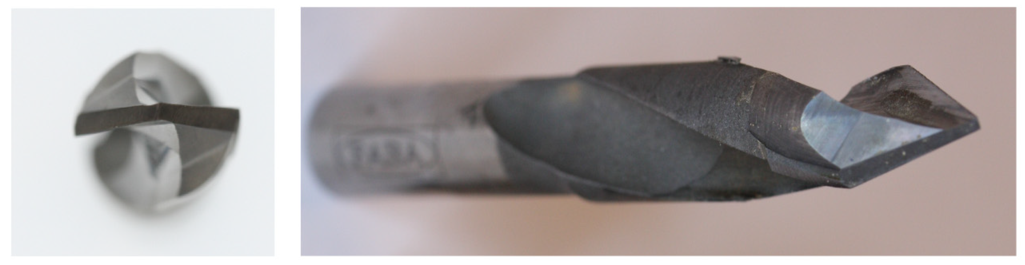
During experimental research, the Computerized Numerical Control (CNC) machining center (Jet 100; Busellato, Thiene, Italy) was used. For the tools, six two-blade drills with diameters of 12 mm were used, with sintered carbide blades (FABA WP–01; Faba SA, Baboszewo, Poland—Figure 1) that are normally used for through-boring in wood-based panels. The holes were made in a three-layer laminated (melamine faced) chipboard (Kronopol U 511 SM; Swiss Krono Ltd., Żary, Poland) at a spindle speed of 4500 rpm and a feed speed of 1.35 m/min (in accordance with the drill bit manufacturer’s recommendations).
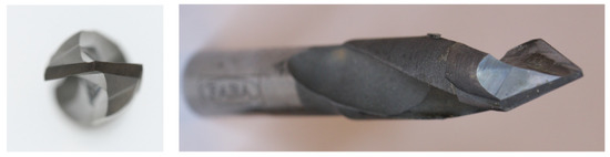
Figure 1.
General view of the drill used in the experiments (FABA WP—01).
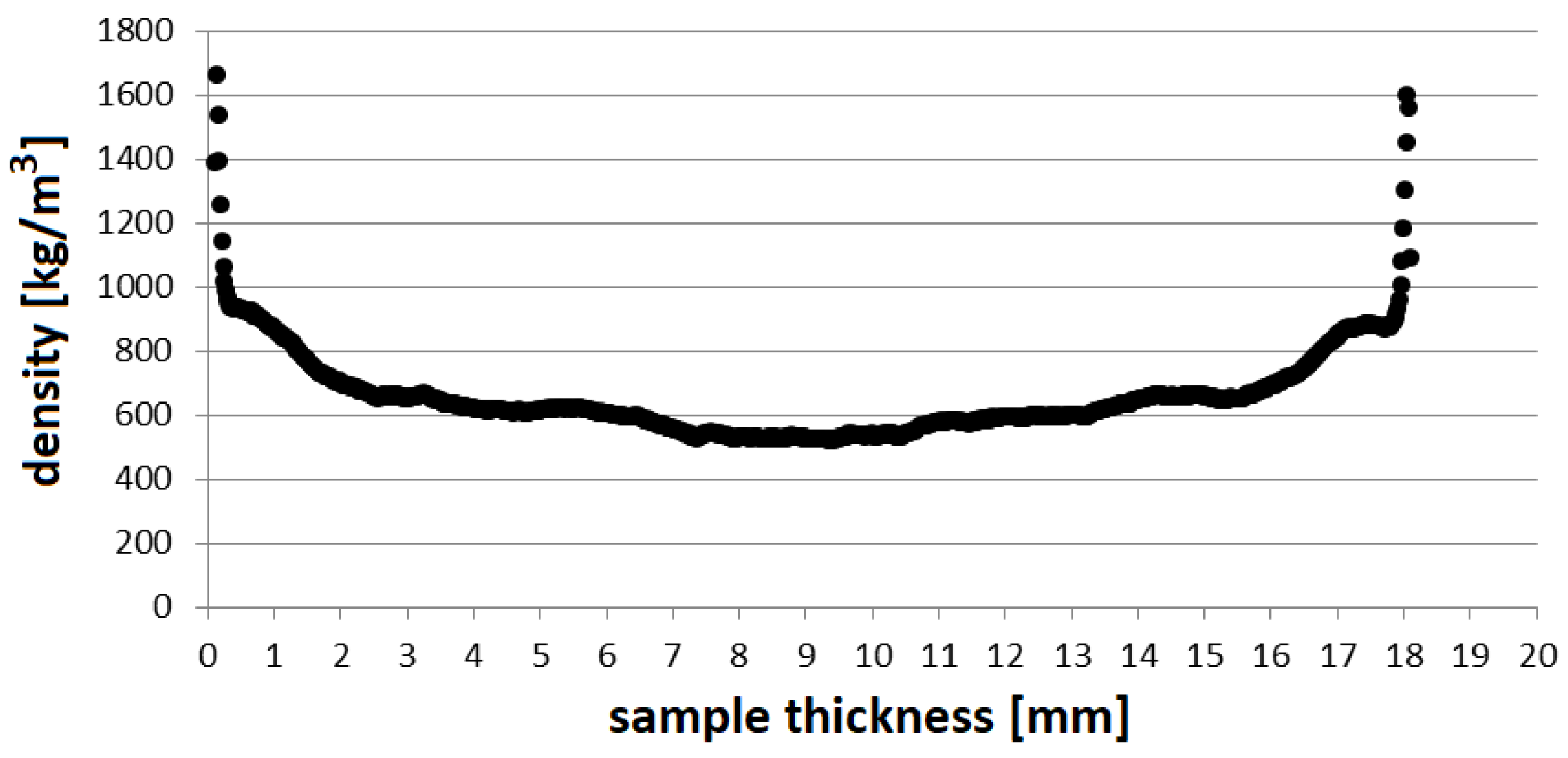
A density profile of the chipboard was determined using a GreCon DAX device (Fagus-GreCon Greten Gmbh & Co. KG, Alfeld, Germany) and is shown in Figure 2. Other material parameters were as follows: the bending modulus of rupture was 15.4 MPa; the bending modulus of elasticity was 2950 MPa; and the surface Brinell hardness (HB) was 2.1. The material tests were performed according to [23,24] using an Instron 3382 (Instron, Norwood, MA, USA) testing machine and a Brinell CV 3000LDB tester (Bowers Group – UK, Camberley, UK), respectively.
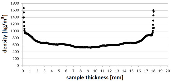
Figure 2.
Density profile of the chipboard used in experiments.
To measure the signals generated in the cutting zone and those constituting the basis for the automatic identification of the condition of tools, a few measurement channels were created, in which the following elements were used:
- Contact sensor of acoustic emission (AE) signal (Kistler 8152B; Kistler Group, Winterthur, Switzerland), which was mechanically pressed against the workpiece;
- Accelerometer for vibration measurement (Kistler 8141B; Kistler Group, Winterthur, Switzerland), which was mounted to the sample holder (jig);
- Force gauge based on 2-component sensor (Kistler 9345A; Kistler Group, Winterthur, Switzerland) for the simultaneous measurement of feed force as well as machining torque;
- Microphone for noise (acoustic pressure) measurement (B&K 4189; Brüel and Kjær, Nærum, Denmark) mounted on the stand near the machining zone.
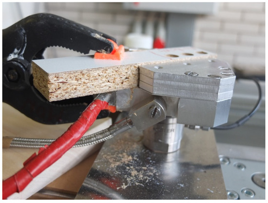
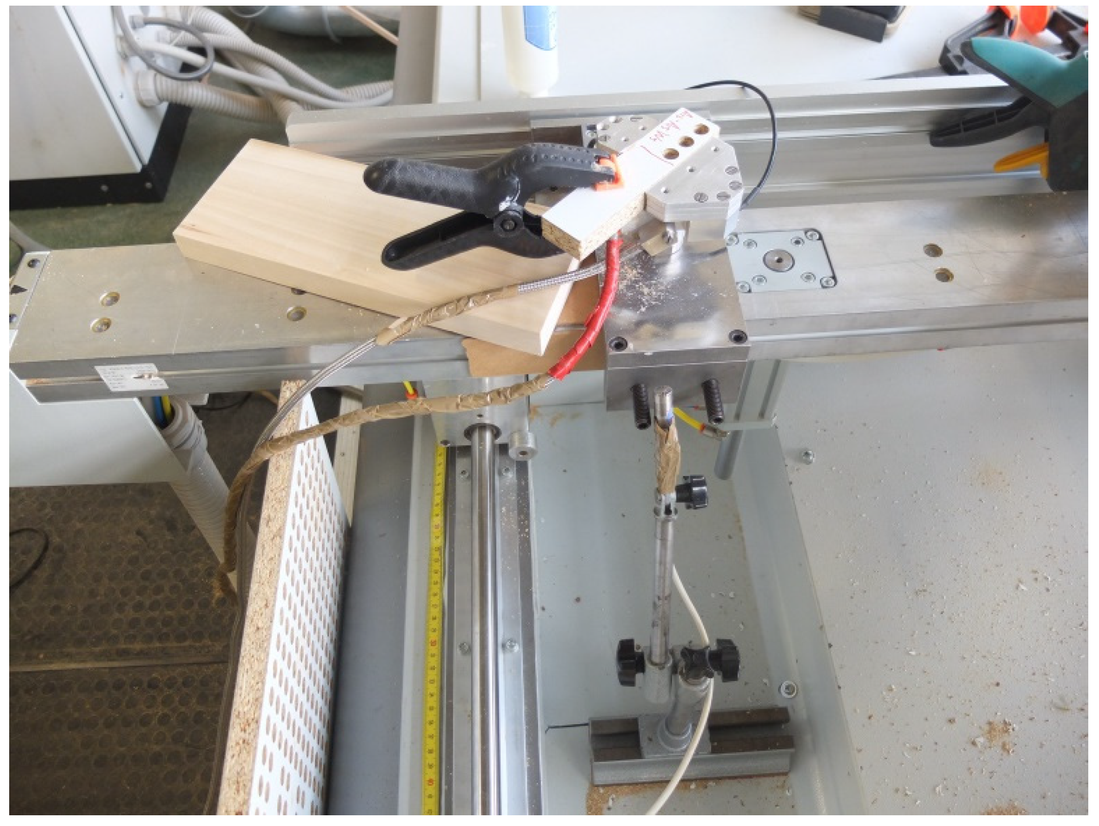
Figure 3.
A detailed view of the workpiece (clamping on a piezoelectric dynamometer), acoustic emission sensor (fixed with a flexible carpentry clamp) and the accelerometer (fixed with a screw).

Figure 4.
A general view of the workpiece (clamping on a piezoelectric dynamometer) and the microphone (mounted on the stand near the machining zone).
The signal sampling was performed in the NI LabVIEW (National Instruments Corporation, ver. 2015 SP1, Austin, TX, USA) environment using two data acquisition cards: NI PCI—6034E and NI PCI—6111 (Austin, TX, USA). The use of two cards was necessitated by the occurrence of signals with different frequencies. The AE signal sampling required the use of a relatively high sampling frequency, 2 MHz, and other signals were registered at a frequency of 50 kHz.
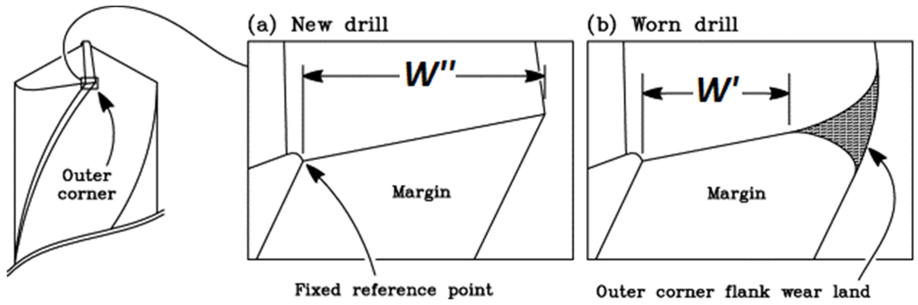
The real condition of drill bits was (for the purpose of further learning and testing, the MLP network effectiveness) directly monitored and assessed using a standard workshop microscope (TM—505; Mitutoyo, Kawasaki, Japan) with a digital camera. As a direct indicator of the condition of the drill bits, the amount of wear (abrasion) of the outer (periphery) corner was assumed. The amount of wear (W) was separately determined for each of the two drill cutting edges, according to the following equation:
where W″ is the initial width of a brand-new cutting edge near the outer corner (mm) (Figure 5), and W′ is the current width of a brand-new cutting edge near the outer corner (mm) (Figure 5).
W = W″ − W′
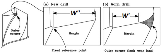
Figure 5.
The method for tool wear measurement: (a) view of a brand new tool, (b) view of worn tool [25].
The general condition of the drill bit was assessed based on the arithmetic mean of the wear of two of its cutting edges, i.e., the average value of the W index.
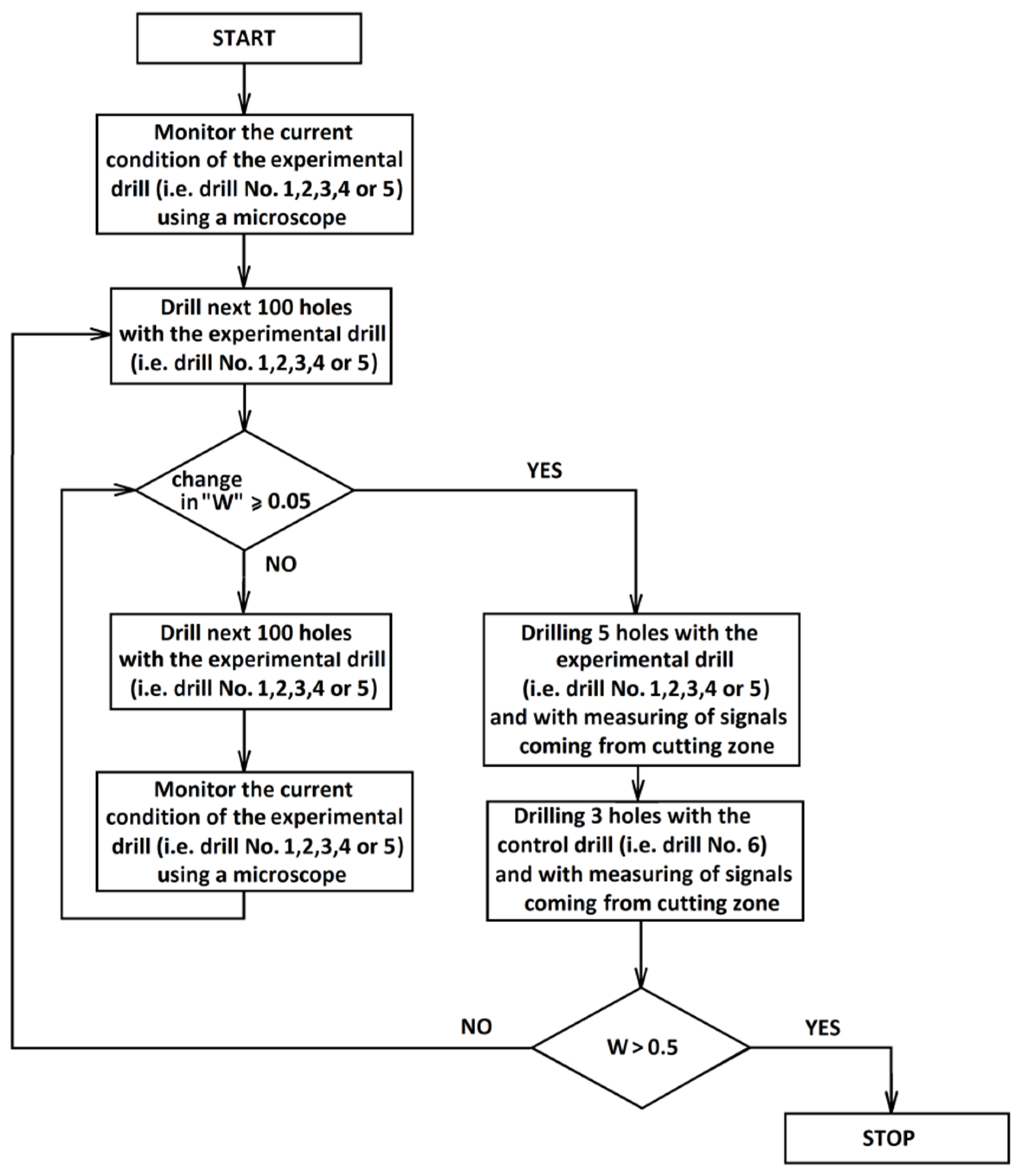
Five of the six drill bits used for the experiment were subjected to operating cycles outside the measuring stand, which gradually changed their initial brand-new condition (W = 0 mm) to the end of the tool life condition (W ≥ 0.5 mm). Each operating cycle consisted of making holes in the laminated particleboard until the drill bit wear was increased by a minimum of 0.05 mm (the number of holes thus varied and ranged from 100 to 300). The number of such cycles was usually 8, but one of the drill bits wore out faster than the others, and, in this case, only 7 cycles were performed. After each such cycle, the drill bit returned to the measuring stand to make a series of 5 holes along with the measuring of the aforementioned signals generated in the cutting zone. Then, the signals accompanying the drilling of three holes with the control drill bit (i.e., the 6th drill bit) were recorded. The sixth drill bit was used as the control tool, and therefore, it was used only to record signals on the measuring stand, i.e., it was not subjected to any operating cycles.
The detailed experimental schedule is presented in a standard flowchart (algorithm diagram) and is shown in Figure 6. The experimental procedure is presented in this figure in a metaphorical form (as if it was an algorithm of a computer program and not a procedure performed by a human being).
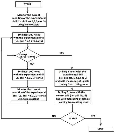
Figure 6.
The experimental schedule as a standard flowchart in a metaphorical form (as if it was an algorithm of a computer program and not a procedure performed by a human being).
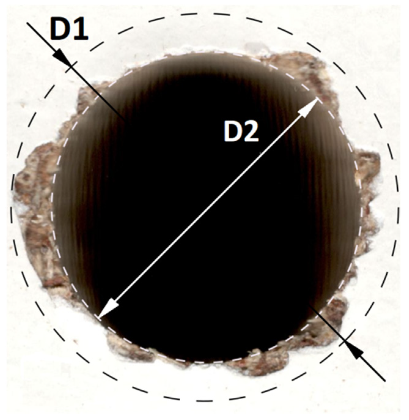
During the experimental research, both tool wear and drilling quality were monitored. The main problem with respect to quality during melamine-faced-wood-based board machining is delamination. Objective delamination monitoring requires an adoption of some sort of a delamination factor [1,2,3,4]. In this case, the delamination factor (Fd) was calculated for each hole (drilled in an experimental workpiece) according to the following equation:
where D1 stands for the diameter of the smallest circle containing the delamination zone (mm) (Figure 7), and D2 stands for the diameter of the largest circle inscribed in the outline of the hole (mm) (Figure 7).
Fd = 0.5·(D1 − D2)

Figure 7.
Delamination factor (Fd) calculation method. The circles with a diameter of D1 and D2 are drawn with a black and white dotted line, respectively.
Both of these diameters (D1 and D2) were determined automatically using computer image analysis based off of scans (1200 dpi) of all experimental workpieces taken with a standard office scanner.
In creating the system for the automatic identification of tool conditions, it was considered that there was no practical need to estimate the current W value. Distinguishing between the three different classes of tool conditions was ultimately of greater importance. The classes are described in this article conventionally as “Green”, “Yellow” and “Red” (analogous to traffic rules). The “Green” class means that the tool is suitable for further work. However, even a single “Yellow” or “Red” class signal made by the diagnostic system means that the tool is not suitable for further work and must be replaced with a new one. The “Yellow” class represents excessive (but not extreme) tool wear. The “Red” class is reserved for extremely worn tools. Definitions of these classes are based on appropriate ranges of W values (Table 1). The upper limit of the “Green” class (0.2 mm), which is crucial from a practical point of view, was suggested by the drill production company. The second limit (0.35 mm, a border between the “Yellow” and “Red” class) was adopted arbitrarily to distinguish “worn” and “completely worn-out” tools in a formal way.

Table 1.
Classes of tool conditions.
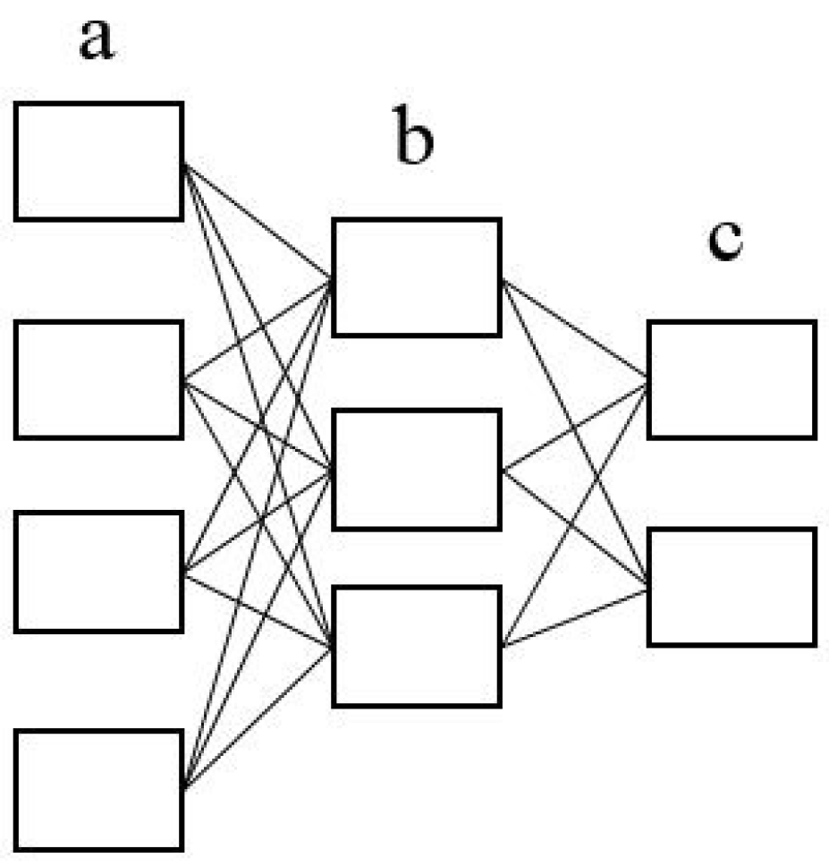
As part of the research task, a standard MLP algorithm was adopted. The MLP network is one of the best-known neural networks [26]. It consists of several neuron layers, and the transmission of the signal between neurons takes place in one direction, starting from the input layer and going through hidden layers to the output layer, where the signal is interpreted. The general structure of two-layer MLP neural network is shown in Figure 8. There can be any number of hidden layers. Neurons connect with each other by means of synapses. Weights—numerical values—are associated with synapses. The weights influence the modification of the values of signals transmitted by neurons in individual layers during network learning. The purpose of the modification of the weights is to obtain the best possible discrimination of samples that reach the input field, i.e., the entry. The weights are an important element of the network because they are responsible for the knowledge it collects. As a result of the weights of synapses, the input information is developed and leads to the classification result. The neuron with a greater weight, when transmitting the signal to the next layer, causes the signal to have an advantage over others. Therefore, as the weight value increases, the variable becomes more important.
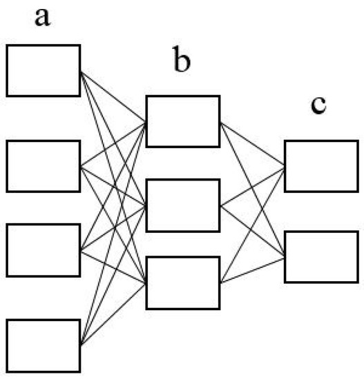
Figure 8.
The general structure of the two-layer MLP neural network: a, input layer; b, hidden layer; c, output layer.
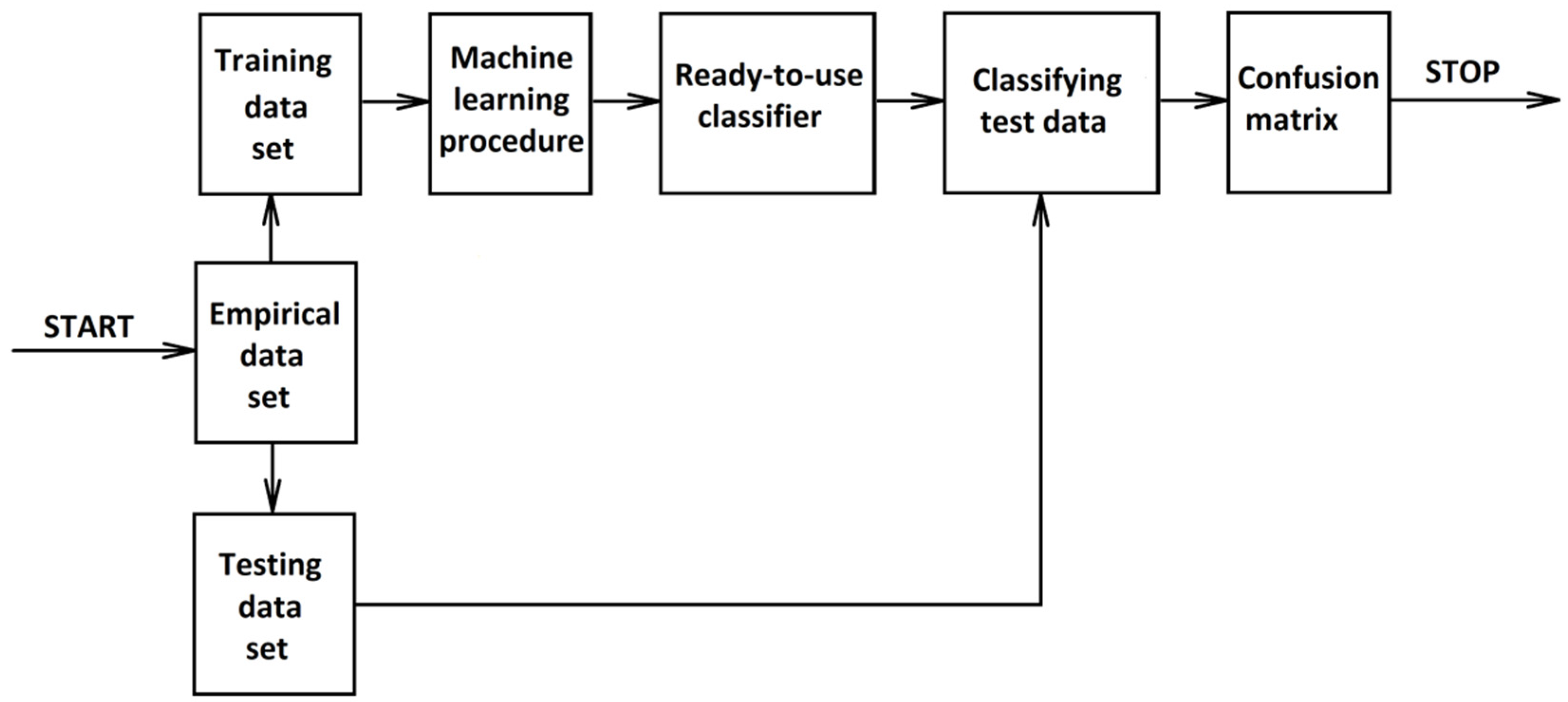
The basic factor determining the operation of the MLP network is learning, and not the structure itself. Therefore, the standard procedure of learning and testing the identification system was adopted (Figure 9).

Figure 9.
The standard procedure of learning and testing the identification system.
First, the “test data” and “training data” sets were created. The “test data” set only included the features of signals registered on the measuring stand with the participation of one drill bit specified as a “test drill” (it was one of the five experimental drills, which had not been used to create the “training data” set). All features used in the study (455 features in total) were extracted using standard functions available in the MATLAB Signal Processing Toolbox and Wavelet Toolbox (MathWorks, Natick, MA, USA). They were standard statistical parameters (such as arithmetic mean, root mean square, variance, skewness, kurtosis, frequencies on histograms etc.) and parameters calculated using wavelet packet transform. The “training data” included the database of five other drill bits (i.e., four other experimental drills and the control drill), which covered both their real, actual classes of tool conditions (“Green,” “Yellow” or “Red”) and features of all signals registered with their participation on the measuring stand. Then, the MLP algorithm was activated in order to identify the current condition of the “test drill” based only on the features of signals included in the “test data” set.
Five different options of the “test data” (including, one by one, each of the five experimental drills) were set up. Thus, five separate tests were performed, but only one total confusion matrix was determined.
Moreover, nine variants of MLP network architectures were tried (Table 2), as described above.
Table 2.
Nine variants of MLP network architectures.
On this basis, for each MLP network structure option, one confusion matrix with a standard structure (Table 3) was generated. The rows correspond to the decisions made by the classifier (predicted classes). Columns, on the other hand, are real classes. The confusion matrix thus shows the relationship between the classified set (predicted classes) and the reference set (real classes) and is the standard basis for assessing the efficiency of the classifier.
Table 3.
Standard structure of the confusion matrix in percentage form.
In this type of matrix, data from outside the diagonal (different than KGG, KYY and KRR) show the mismatch between the predicted class and the real one, i.e., incorrect classifications. For example, KGY means the percentage of observations calculated as the ratio of the count of true “Green” observations incorrectly assigned to the “Yellow” class to the total observation count. The most disturbing were considered non-zero KRG and KGR values, which testified about cases of confusion between “Green” and “Red” or vice versa.
The sum of properly classified percentages of samples (i.e., the sum of the percentages that can be read on the diagonal of the matrix) represents the overall accuracy (Acco) of the classification according to the following equation:
where KGG + KYY + KRR equals the percentage of samples classified correctly (the percentage of right decisions made by the classifier).
For each class, separately, the following parameters were also determined:
- TP: the number of true positive predictions;
- TN: the number of true negative predictions;
- FP: the number of false positive predictions;
- FN: the number of false negative predictions.
On this basis, five standard, detailed indicators of the effectiveness of its identification by the MLP network were calculated for each class separately:
The first of them was sensitivity (Sn):
The second was specificity (Sp):
The third was precision (Pr):
The fourth was accuracy (Acc):
The fifth was the harmonic mean of precision and sensitivity (Fscore):
It is worth noting that the maximum level of each of the aforementioned indicators (showing the flawless operation of the classifier) is the number 1.
All numerical calculations and data mining analyses were carried out in the MATLAB environment.
3. Results and Discussion
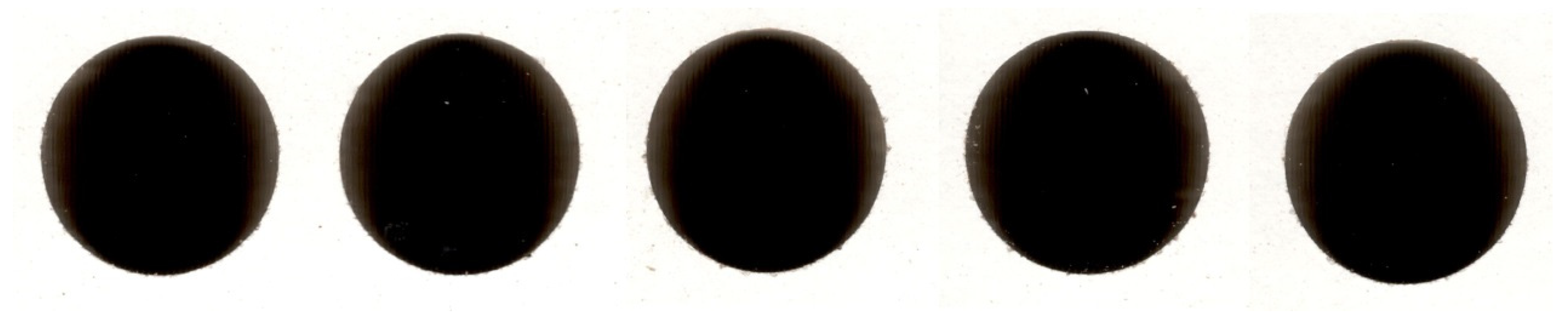
Firstly, the machining quality (hence the delamination problem) was analyzed. The sample holes made with drills representing three different tool wear classes are shown in Figure 10, Figure 11 and Figure 12.
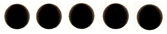
Figure 10.
The sample holes made with relatively sharp drills. (“Green” tool wear class—W < 0.2 mm).
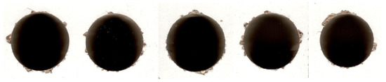
Figure 11.
The sample holes made with drills representing excessive (but not extreme) tool wear (“Yellow” tool wear class—0.2 ≤ W < 0.35 mm).
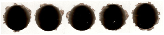
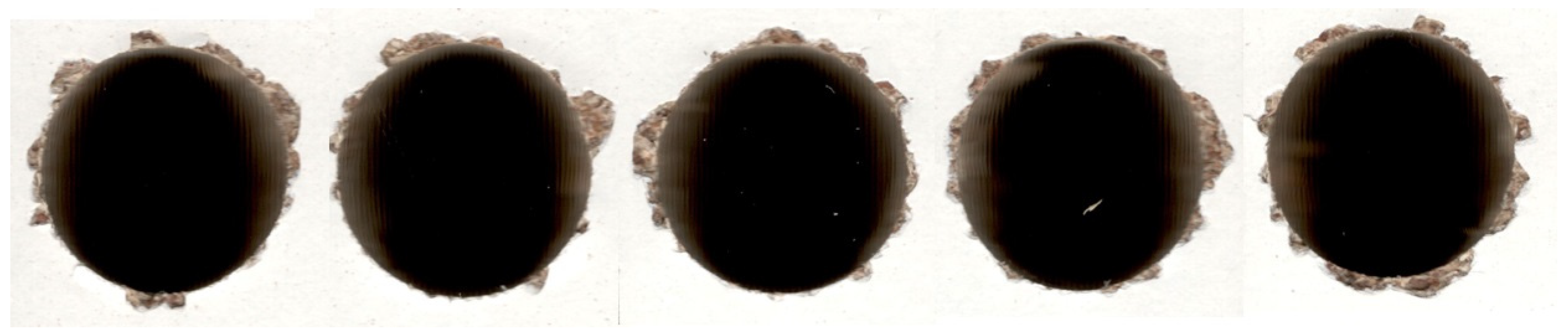
Figure 12.
The sample holes made with completely worn-out drills (“Red” tool wear class—0.35 ≤ W).
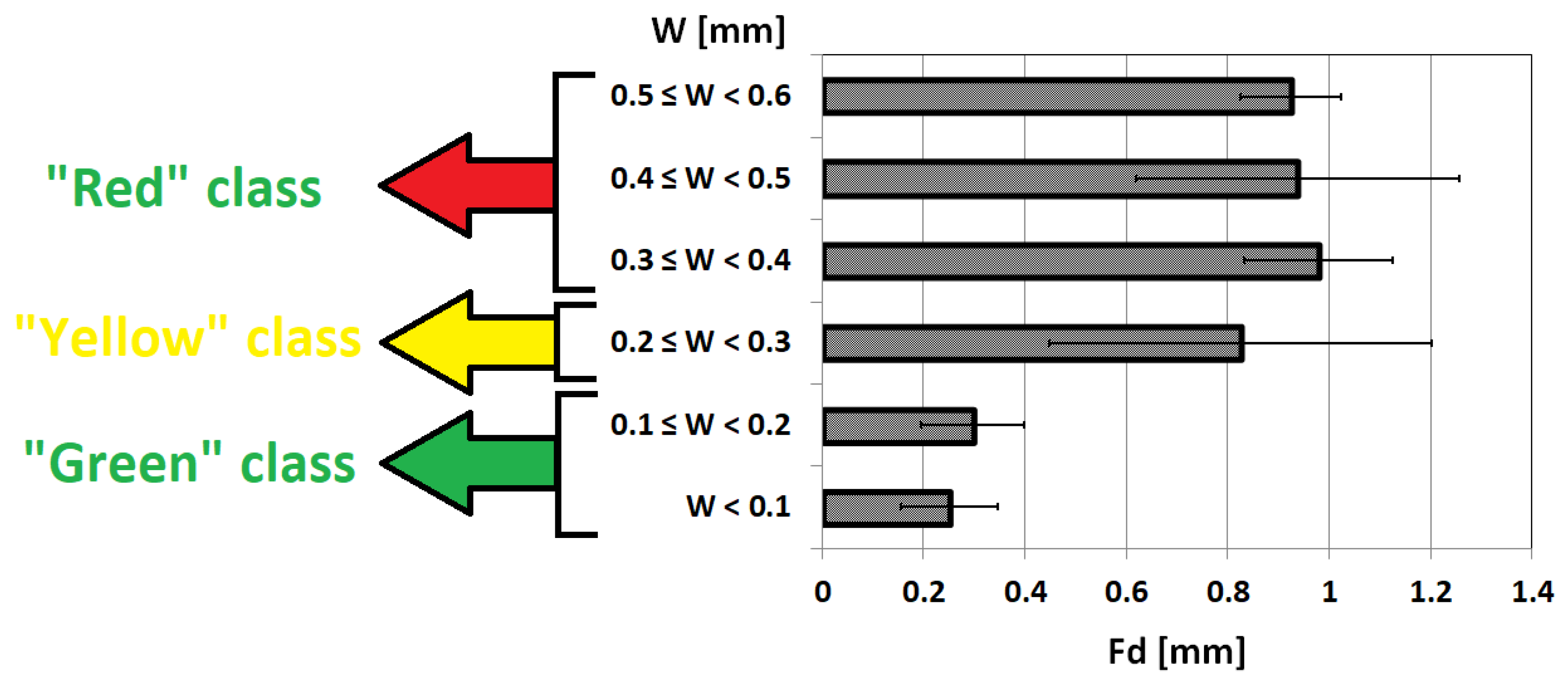
Figure 13 shows the statistical relationship between the degree of tool wear (W index) and the delamination factor (Fd). Ultimately, the drilling quality in the “Green” class (W < 0.2 mm) was clearly better and more stable than in the other two classes (W ≥ 0.2). This confirmed the legitimacy (practical utility) of the tool wear limit suggested by the drill production company.

Figure 13.
The values of delamination factor (Fd) in different classes of tool wear.
Next, as a part of the research project, different MLP network architectures were built and tested (according to Table 2). Based on comparisons of their overall effectiveness, the best one (the most effective) was chosen. Ultimately, the most effective network consisted of 3 hidden layers, and each layer contained 15 neurons. According to the classification results, further increases in the number of neurons in the layers and the number of layers themselves resulted in the deterioration of the classification accuracy. The expansion of the network did not give a positive effect. The quality of the classification for the best MLP network option is illustrated by the percentage matrix confusion in Table 4. The general idea of this table is the same for Table 3, which was described earlier. The overall accuracy (Acco) of the classification was ultimately more than 70%, which can be calculated using Formula (3). This result is generally decent but slightly worse than that of the classification algorithms tested earlier (“support vector machine” [20] and “nearest neighbors” [21] algorithms). The most troublesome, however, is the fact that (as shown in Table 4) serious errors (mistakes between “Green” and “Red” classes) were occasionally noted. More specifically, the MLP network twice classified the “Red” tool as a “Green” tool, which was 0.9% of the whole set classification. In contrast, it was advantageous that there was never a reverse mistake.
Table 4.
Confusion matrix for the best variant of MLP structure.
Table 5 contains detailed indicators of the effectiveness of the identification of individual classes of tool conditions by the best MLP network. The table shows that the Acc, Sn and Fscore parameters had the greatest values (0.85, 0.89 and 0.82, respectively) for the “Red” class, which shows that the classifier best recognized samples belonging to this class and most effectively separated them from the others. For the “Green” class, the aforementioned parameters also had relatively high values (0.84, 0.75 and 0.77, respectively). Moreover, it was the “Green” class that had the best values of Sp and Pr parameters (0.89 and 0.79, respectively). Good recognition of this class was shown. In the case of the “Yellow” class, however, the obtained results were by far the worst, because this class is adjacent to both the “Green” and “Red” classes, and the degree of wear and tear defined in Table 1 clearly shows that the difference between them was not big, making it difficult to separate neighboring classes.
Table 5.
Detailed indicators of the effectiveness of identification of individual classes of tool conditions.
4. Conclusions
- The classification effects (with an overall accuracy above 70%) were ultimately fairly decent but slightly worse than those of the classification algorithms tested earlier (i.e., “nearest neighbors” or “support vector machine” algorithms). The most troublesome, however, is the fact that serious errors (mistakes between extreme classes “Green” and “Red”) were occasionally noted (for about 1% of the analyzed cases).
- The most important and the best news is that the “Green” class (which is the most important one from a practical point of view) was identified quite accurately (accuracy: 0.84; Fscore: 0.77). This is very beneficial because the main job of the tool condition monitoring system is to identify tools which should not yet be changed.
- Thinking about future research, we plan to consider the drilling of various wood-based materials (e.g., MDF), testing other classification algorithms and analyzing the problem of selecting signal features for their usefulness.
Author Contributions
Conceptualization, A.J., J.K., M.K. and J.G.; methodology, J.K., M.K. and J.G.; validation, J.K. and M.K.; formal analysis, A.J., J.K. and M.K.; investigation, A.J.; resources, J.K., M.K. and A.J.; data curation, A.J. and J.K.; writing—original draft preparation, J.G.; writing—review and editing, A.J. and J.G.; visualization, A.J.; supervision, A.J. and J.K.; project administration, A.J.; funding acquisition, J.G. All authors have read and agreed to the published version of the manuscript.
Funding
This work was supported by the Polish State Committee for Scientific Research (Grant No. P06L02524).
Institutional Review Board Statement
Not applicable.
Informed Consent Statement
Not applicable.
Data Availability Statement
The data presented in this study are available in the article. Additional data are available on request from the corresponding author.
Acknowledgments
The authors gratefully acknowledge funding from the Polish State Committee for Scientific Research.
Conflicts of Interest
The authors declare no conflict of interest.
References
- Kun, W.; Qi, S.; Cheng, W. Influence of pneumatic pressure on delamination factor of drilling medium density fiberboard. Wood Res. 2015, 60, 429–440. [Google Scholar]
- Szwajka, K.; Trzepieciński, T. Effect of tool material on tool wear and delamination during machining of particleboard. J. Wood Sci. 2016, 62, 305–315. [Google Scholar] [CrossRef]
- Szwajka, K.; Trzepieciński, T. An examination of the tool life and surface quality during drilling melamine faced chipboard. Wood Res. 2017, 62, 307–318. [Google Scholar]
- Śmietańska, K.; Podziewski, P.; Bator, M.; Górski, J. Automated monitoring of delamination factor during up (conventional) and down (climb) milling of melamine-faced MDF using image processing methods. Eur. J. Wood Wood Prod. 2020, 78, 613–615. [Google Scholar] [CrossRef] [Green Version]
- Lemaster, R.L.; Tee, L.B.; Dornfeld, D.A. Monitoring tool wear during wood machining with acoustic emission. Wear 1985, 101, 273–282. [Google Scholar] [CrossRef]
- Lemaster, R.L.; Lu, L.; Jackson, S. The use of process monitoring techniques on a CNC wood router. Part 1. Sensor selection. For. Prod. J. 2000, 50, 31–38. [Google Scholar]
- Lemaster, R.L.; Lu, L.; Jackson, S. The use of process monitoring techniques on a CNC wood router. Part 2. Use of vibration accelerometer to monitor tool wear and workpiece quality. For. Prod. J. 2000, 50, 59–64. [Google Scholar]
- Zhu, N.; Tanaka, C.; Ohtani, T.; Usuki, H. Automatic detection of a damaged cutting tool during machining I: Method to detect damaged bandsaw teeth during sawing. J. Wood Sci. 2000, 46, 437–443. [Google Scholar] [CrossRef]
- Zhu, N.; Tanaka, C.; Ohtani, T. Automatic detection of damaged bandsaw teeth during sawing. Holz Roh Werkst. 2002, 60, 197–201. [Google Scholar] [CrossRef]
- Zhu, N.; Tanaka, C.; Ohtani, T.; Takimoto, Y. Automatic detection of a damaged router bit during cutting. Holz Roh Werkst. 2004, 62, 126–130. [Google Scholar] [CrossRef]
- Suetsugu, Y.; Ando, K.; Hattori, N.; Kitayama, S. A tool wear sensor for circular saws using wavelet transform signal processing. For. Prod. J. 2005, 55, 79. [Google Scholar]
- Szwajka, K.; Górski, J. Evaluation tool condition of milling wood on the basis of vibration signal. J. Phys. Conf. Ser. 2006, 48, 1205–1209. [Google Scholar] [CrossRef]
- Wilkowski, J.; Górski, J. Vibro-acoustic signals as a source of information about tool wear during laminated chipboard milling. Wood Res. 2011, 56, 57–66. [Google Scholar]
- Górski, J.; Szymanowski, K.; Podziewski, P.; Śmietańska, K.; Czarniak, P.; Cyrankowski, M. Use of cutting force and vibro-acoustic signals in tool wear monitoring based on multiple regression technique for compreg milling. BioResources 2019, 14, 3379–3388. [Google Scholar] [CrossRef]
- Nasir, V.; Cool, J.; Sassani, F. Intelligent Machining Monitoring Using Sound Signal Processed With the Wavelet Method and a Self-Organizing Neural Network. IEEE Trans. Robot. Autom. 2019, 4, 3449–3456. [Google Scholar] [CrossRef]
- Nasir, V.; Sassani, F. A review on deep learning in machining and tool monitoring: Methods, opportunities, and challenges. Int. J. Adv. Manuf. Technol. 2021, 115, 2683–2709. [Google Scholar] [CrossRef]
- Zbieć, M. Application of Neural Network in Simple Tool Wear Monitoring and Indentification System in MDF Milling. Drv. Ind. 2011, 62, 43–54. [Google Scholar] [CrossRef]
- Tratar, J.; Pušavec, F.; Kopac, J. Tool wear in terms of vibration effects in milling medium-density fibreboard with an industrial robot. J. Mech. Sci. Technol. 2015, 28, 4421–4429. [Google Scholar] [CrossRef]
- Nasir, V.; Dibaji, S.; Alaswad, K.; Cool, J. Tool wear monitoring by ensemble learning and sensor fusion using power, sound, vibration, and AE signals. Manuf. Lett. 2001, 30, 32–38. [Google Scholar] [CrossRef]
- Jegorowa, A.; Górski, J.; Kurek, J.; Kruk, M. Initial study on the use of support vector machine (SVM) in tool condition monitoring in chipboard drilling. Eur. J. Wood Wood Prod. 2019, 77, 957–959. [Google Scholar] [CrossRef] [Green Version]
- Jegorowa, A.; Górski, J.; Kurek, J.; Kruk, M. Use of nearest neighbors (k-NN) algorithm in tool condition identification in the case of drilling in melamine faced particleboard. Maderas-Cienc. Tecnol. 2020, 22, 189–196. [Google Scholar] [CrossRef] [Green Version]
- Górski, J. The Review of New Scientific Developments in Drilling in Wood-Based Panels with Particular Emphasis on the Latest Research Trends in Drill Condition Monitoring. Forests 2022, 13, 242. [Google Scholar] [CrossRef]
- EN 310; Wood-Based Panels: Determination of Modulus of Elasticity in Bending and of Bending Strength. CEN: Brussels, Belgium, 1994.
- EN 1534; Wood Flooring and Parquet: Determination of Resistance to Indentation—Test Method. CEN: Brussels, Belgium, 2002.
- Czarniak, P.; Szymanowski, K.; Panjan, P.; Górski, J. Initial Study of the Effect of Some PVD Coatings (“TiN/AlTiN” and “TiAlN/a-C:N”) on the Wear Resistance of Wood Drilling Tools. Forests 2022, 13, 286. [Google Scholar] [CrossRef]
- Haykin, S. Neural Networks: A Comprehensive Foundation; Macmillan College Publishing Company, Inc.: New York, NY, USA, 1994. [Google Scholar]


Publisher’s Note: MDPI stays neutral with regard to jurisdictional claims in published maps and institutional affiliations. |
© 2022 by the authors. Licensee MDPI, Basel, Switzerland. This article is an open access article distributed under the terms and conditions of the Creative Commons Attribution (CC BY) license (https://creativecommons.org/licenses/by/4.0/).