Vegetation Type Classification Based on 3D Convolutional Neural Network Model: A Case Study of Baishuijiang National Nature Reserve

Abstract

Efficient and accurate vegetation type extraction from remote sensing images can provide decision makers with basic forest cover and land use information, and provides a reliable basis for long-term monitoring. With the development of deep learning, the convolutional neural network (CNN) has been used successfully to classify tree species in many studies, but CNN models have rarely been applied in the classification of vegetation types on larger scales. To evaluate the performance of CNN models in the classification of vegetation types, this paper compared the classification accuracy of nine dominant land cover types in Baishuijiang National Nature Reserve with four models: 3D-CNN, 2D-CNN, JSSAN (joint spatial–spectral attention network) and Resnet18, using sentinel-2A data. Comparing the difference in classification accuracy between the direct use of raw sentinel images and fused feature indices sentinel images, the results showed that adding feature indices can improve the overall accuracy of the model. After fusing the characteristic bands, the accuracy of the four models was improved significantly, by 5.46–19.33%. The best performing 3D-CNN model achieved the highest classification accuracy with an overall accuracy of 95.82% and a kappa coefficient of 95.07%. In comparison, 2D-CNN achieved an overall accuracy of 79.07% and a kappa coefficient of 75.44%, JSSAN achieved an overall accuracy of 81.67% and a kappa coefficient of 78.56%, and Resnet18 achieved an overall accuracy of 93.61% and a kappa coefficient of 92.45%. The results showed that the 3D-CNN model can effectively capture vegetation type cover changes from broad-leaved forests at lower elevation, to shrublands and grasslands at higher elevation, across a range spanning 542–4007 m. In experiments using a small amount of sample data, 3D-CNN can better incorporate spatial–spectral information and is more effective in distinguishing the performance of spectrally similar vegetation types, providing an efficient and novel approach to classifying vegetation types in nature reserves with complex conditions.

1. Introduction

Vegetation plays an crucial role in maintaining the material and energy balance, and stability of terrestrial ecosystems. It provides a reliable guarantee of human survival and development [1,2]. The extraction of vegetation types can provide decision makers with basic forest cover and land use information, and provides a robust basis for long-term monitoring.

The traditional method of vegetation type classification is based on manual visual interpretation, which requires extensive field surveys and a high level of researcher experience in remote sensing and botany. Therefore, it is difficult to apply in large area vegetation type extraction. With the development of remote sensing technology, more and more images have high spatial and temporal resolution, and machine learning methods have gradually replaced traditional methods. Methods such as the support vector machine, random forest, decision tree, multilayer perceptron and artificial neural network have been used in the field of agroforestry, urban vegetation, tropical rainforests and land use cover [3,4,5,6,7,8] to classify dominant feature types, achieving 70–91% accuracy. However, machine learning methods applied to vegetation classification usually require complex preparatory work [9]. In contrast, the end-to-end learning approach in deep learning can automatically extract important features, thereby reducing manual intervention [10].

A convolutional neural network (CNN) is a feed-forward neural network, which mainly consists of convolutional, pooling and fully connected layers. The LeNet-5 model is the first true CNN model that enabled the classification of handwritten numbers [11]. Subsequently, more work improved the network. Classical models include AlexNet [12], where Relu is used as an activation function instead of Sigmoid, to solve the gradient dispersion problem when the network is deeper; VGGNet [13], which uses convolutional layers composed of multiple small convolutional kernels instead of larger convolutional layers to reduce the parameters and also to increase the nonlinear fitting ability; and ResNet [14], in which the residual structure solves the gradient disappearance problem with the deep convolutional layers. The development of CNN has contributed greatly to computer visualization and image classification, and has also provided excellent portable models for vegetation classification.

The U-net model was used to map woody vegetation in Queensland, Australia [15], reaching 90% accuracy and demonstrating the suitability of CNN models for woody vegetation mapping in large regions. Convolutional operations are essentially computed based on the local perceptual field generated by the convolutional kernel, which limits the overall understanding of complex scenes, while the attention mechanism can aggregate local information, suppress the worthless information, and obtain a global–local connection. Related works made full use of local and global information to explain complex natural scenes by using a point-by-point spatial attention mechanism to unite contextual dependencies [16]. CNN can improve the learning ability of the model by adding a spatial attention mechanism and a cascaded residual module, and the fusion model has significantly improved the land cover classification accuracy in a high-resolution land cover dataset [17,18,19]. Due to the rich information of spectral dimension of hyperspectral data, further development has introduced 3D-CNN to jointly extract spatial–spectral features [20]. The 3D convolution kernel can extract local information flow in cubic space and spectral dimension, and use the important features to participate in classification [10].

Adding informative features of the original image in a limited training sample is also a way to enhance the classification accuracy. For example, recent work [21] preprocessed the raw images and used six multispectral indices to enhance the training information and to improve the extraction accuracy of mangroves. Many studies have used a combination of the normalized difference vegetation index (NDVI) and texture features to enhance vegetation classification [22,23,24]. NDVI can enhance phenological differences between vegetation types [25], and texture reflects homogeneity in images to improve classification by enhancing homogeneity and preserving the boundaries of elements of the same types [26]. Other studies [4,27] found that band textures in the near-infrared and short-wave infrared regions contributed more to the extraction of canopy edges. Compared with NDVI, the enhanced vegetation index with a soil adjustment factor achieves more accurate performance for vegetation detection in mountainous areas with undulating topography [28,29].

The existing vegetation type classification is limited by study areas, data sources and modeling methods, and it is difficult to achieve the requirements of high precision classification. This is especially true for the majority of the proposed theoretical architectures, which have adopted publicly available datasets with low resolution, clear distinction between classes, and low noise; these include the Indian Pines, Pavia University, and others [30,31,32]. The adaptability of these proposed methods in the relatively complex nature reserves remains to be considered. Therefore, this article selected four different CNN models to explore the ability of 3D convolution kernels to extract spectral space information in the Baishuijiang National Nature Reserve. The objectives of this study are (1) to investigate the influence of vegetation index and elevation data fusion on the accuracy of the model, and (2) to compare the performance of four CNN models (3D-CNN, 2D-CNN, JSSAN, and Resnet18) in the classification of vegetation types.

2. Research Area and Materials

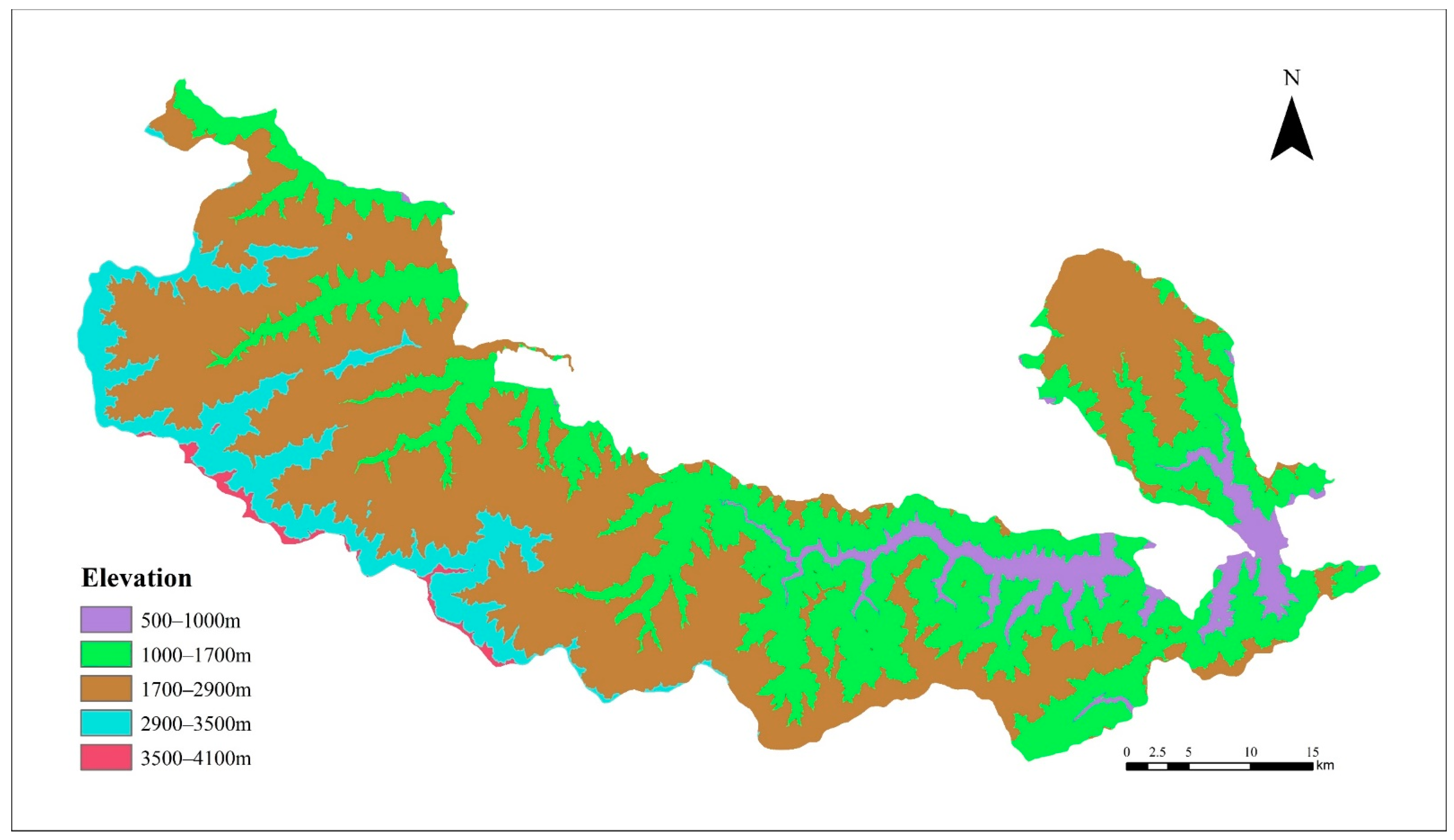
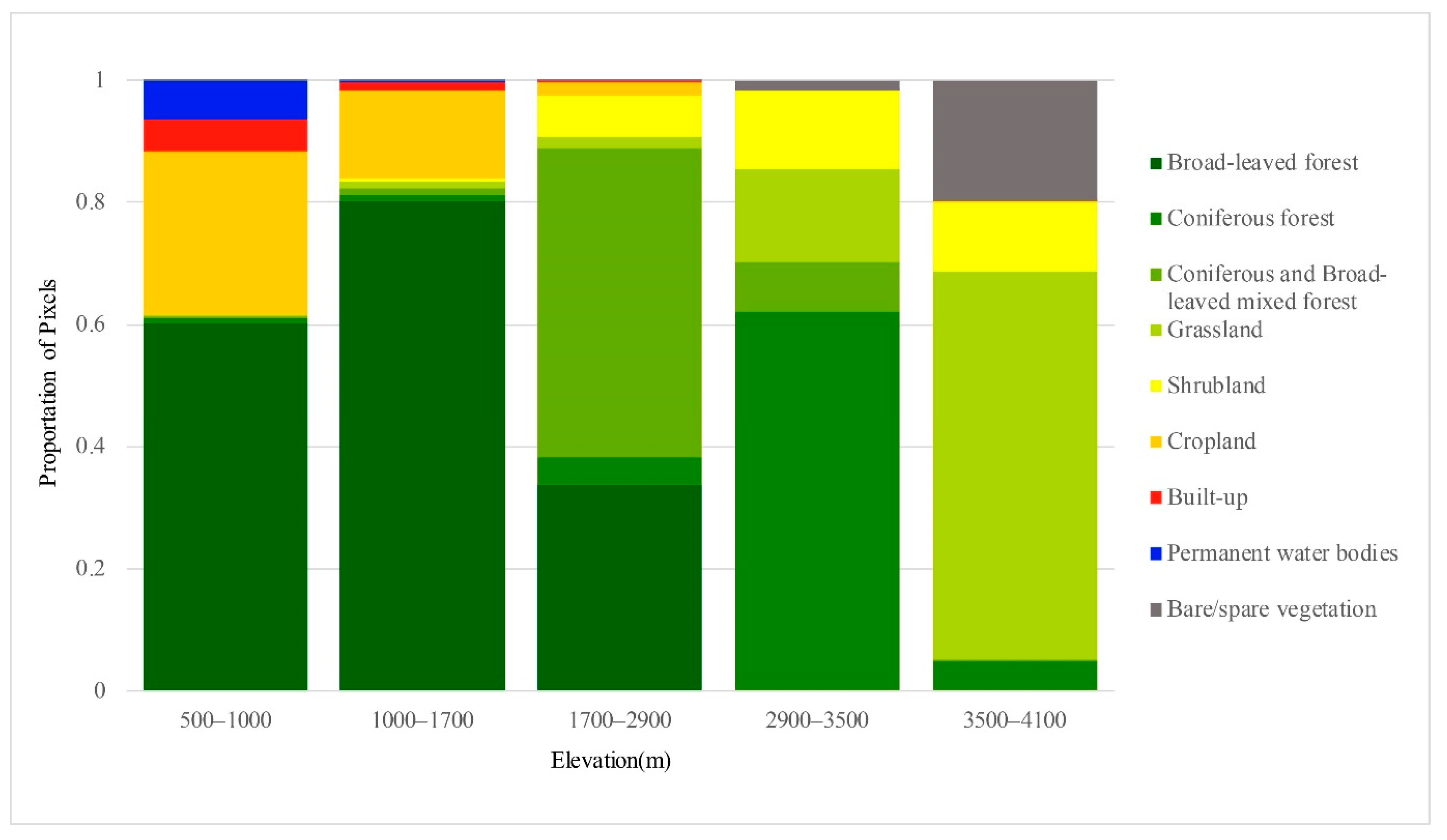
2.1. Research Area

Baishuijiang National Nature Reserve (104°7′~105°22′ E, 32°35′~33°5′ N) was established in 1978. The reserve is located in Longnan City, in the south of Gansu Province (Figure 1), bordering Mianyang City and Guangyuan City of Sichuan Province. The nature reserve covers a total area of 1861.1 km². The main landscape type in the study area is mountainous, and the altitude increases gradually from northeast to southwest, ranging from 542 to 4007 m. According to the basic information of the Baishuijiang Nature Reserve Administration (http://www.baishuijiang.com.cn/ accessed date: 1 March 2021), the vegetation distribution in the nature reserve is vertically zoned, with evergreen broad-leaved forest (<1000 m), mixed evergreen deciduous broad-leaved forest (1000–1700 m), coniferous and broad-leaved mixed forest (1700–2900 m), evergreen coniferous forest (2900–3500 m) and alpine scrub meadow (>3500 m).

The nature reserve belongs to the transition climate zone from the northern subtropics to warm temperate zones, with an average annual precipitation of 800 mm. The humid climate of the north rim of the northern subtropics and high-middle mountain landscape create good conditions for the development of plants, and it is an area with a strong vegetation diversity [33].

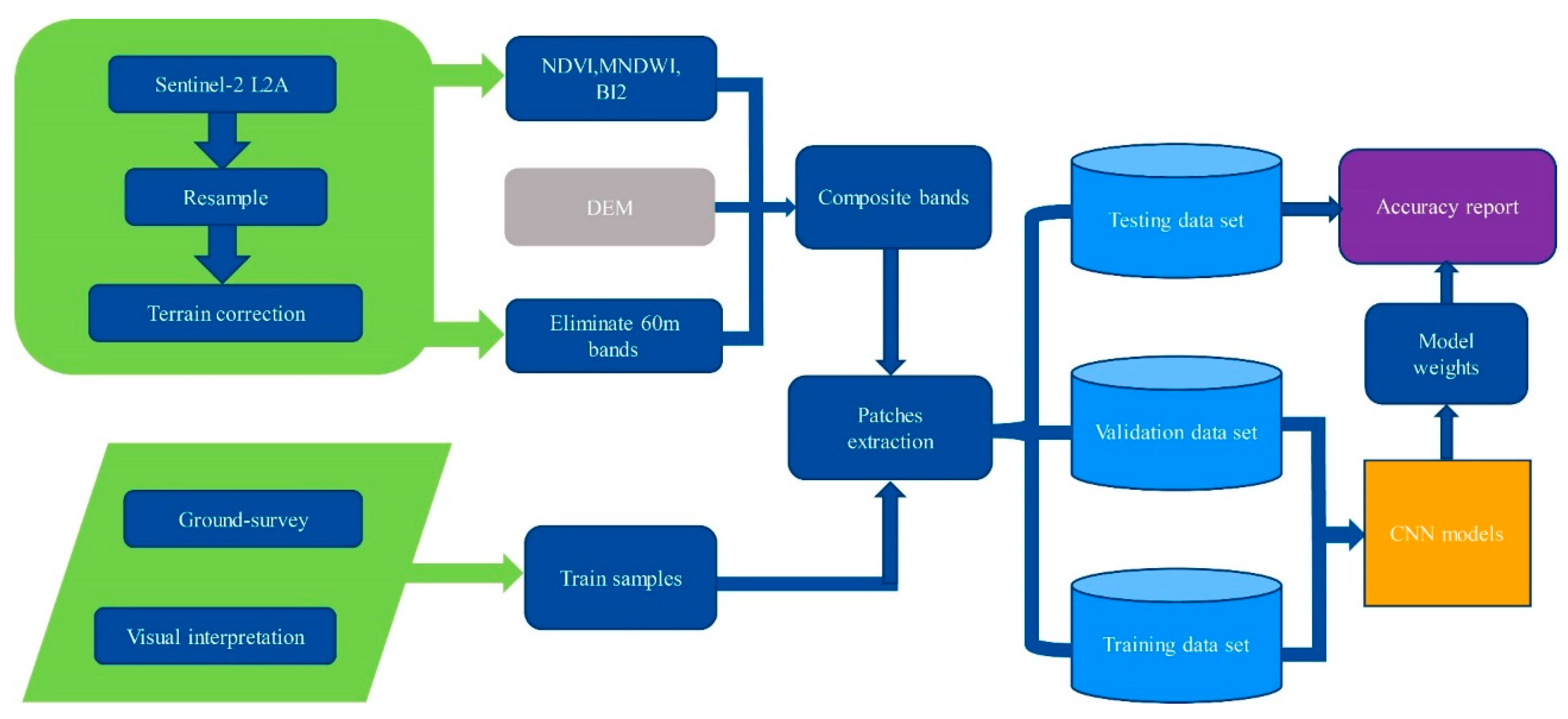
2.2. Data Sources and Pre-Processing

We acquired four Sentinel-2 L2A images to patch the entire study area, using data from different years instead of products with higher cloudiness (https://scihub.copernicus.eu/dhus/#/home accessed date: 1 March 2021). The images were acquired on 15 August 2019, 9 August 2020 (two images) and 29 April 2021, with the final image cloudiness controlled to less than 1%. By using SNAP 8.0.8 software, the 60 m resolution bands (aerosol, water vapor, cirrus) were removed and the remaining bands with different resolutions were resampled to a resolution of 10 m. A topography correction was used to eliminate the variation of image irradiance values due to topographic relief, so that the images could better reflect the spectral characteristics of the features. The spectral indices NDVI, the modified normalized difference water index (MNDWI), and the second brightness index (BI2) were extracted, and then the digital elevation model (DEM) data with a resolution of 12.5 m (resampled to 10 m resolution) of the nature reserve were fused. The final composite image had 14 bands. NDVI is calculated as Equation (1) [34]:

$$\mathrm{NDVI}=\frac{{\rho }_{NIR}-{\rho }_{red}}{{\rho }_{NIR}+{\rho }_{red}}$$

(1)

MNDWI is calculated as Equation (2) [35]:

$$\mathrm{MNDWI}=\frac{{\rho }_{Green}-{\rho }_{MIR}}{{\rho }_{Green}+{\rho }_{MIR}}$$

(2)

Finally, BI2 is calculated as Equation (3) [36]:

$$\mathrm{BI}2=\sqrt{\left({\rho }_{red}^2+{\rho }_{green}^2+{\rho }_{NIR}^2\right)/3}$$

(3)

where ρ_NIR, ρ_red, ρ_green, ρ_MIR in Equations (1)–(3) represent the near infrared, red, green, and the middle infrared reflectance values for a given pixel.

2.3. Sample Selection

The main vegetation community types were determined based on the species cover of the nature reserve. According to the biological resource list of the Baishuijiang Nature Reserve and field survey in the field, the land cover types were classified into nine categories: broad-leaved forest, coniferous forest, coniferous and broad-leaved mixed forest, grassland, shrubland, cropland, built-up, permanent water bodies, and bare/spare vegetation. The sampling plots were defined by the Sentinel-2 and Google images combined with manual interpretation. The actual sampling process mainly used GPS points for labeling samples. The sample size is a regular square of 15 × 15, and a single type accounting for 80% or more is the label value of the sample plot. A total of 1006 regular area samples were selected, which were roughly evenly distributed within the nature reserve as shown in Figure 1.

3. Methods

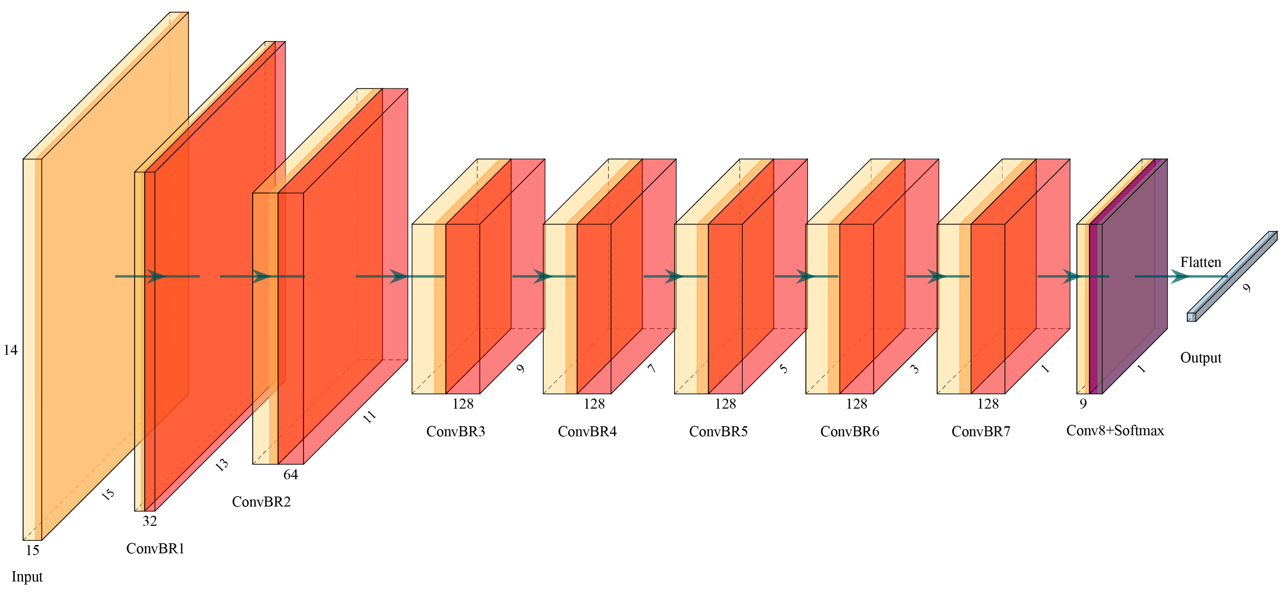
3.1. CNN Model Framework

In this study, a pixel-level 3D-CNN classification framework was constructed. The original image was segmented into several cubic patches of size W × W × B × 1 (where W is the width and height of the patch and B is the number of bands of the multispectral image). The size of the patches can affect the effectiveness of model training; too much input data may introduce additional noise [37], while too little input data may make the receptive field too small to learn more information. The most appropriate patch size setting uses W = 15, based on experience and the multispectral data situation. In joint spatial-temporal feature information, the 3 × 3 × 3 convolution kernel proved to be the best choice in 3D-CNN [38]. The 15 × 15 × 14 spatial cubes go through six layers of convolution operations with 3 × 3 × 3 convolution kernels, with a default step size of 1. The output feature map size then becomes 3 × 3 × 2, and is passed through a layer with 3 × 3 × 2 convolution kernel, resulting in the 1 × 1 × 1 output data. Therefore, the input data can go through, at most, 7 down-sampling convolution operations of that size. The last convolution layer sets the number of channels as nine, in accordance with the nine classification types. Therefore, the 3D-CNN structure of the eight convolutional layers were evaluated as shown in Figure 2. The number of convolution kernels in the network influences its recognition ability, and more convolution kernels imply a network with more learning ability. After the down-sampling processing of each layer, the size of the feature map becomes smaller and more convolution kernels are needed to learn more features [12]. Thus, the next layer has twice as many convolution kernels as the last, until the maximum number of channels is reached. We note that convolution kernels should not be over-expanded either, as this could lead to over-fitting to the training data, and may demand severe computational load [39]. L2 regularization of strength α was applied in the convolution of each layer, where α is an additional hyperparameter. Each convolutional layer (except the last one) uses a normalization function (BatchNormalization) and the flow linear unit (ReLU) [39] to prevent overfitting. The final layer uses the softmax as the activation function to derive the probabilities for each category and then uses the argmax function to predict the final classification result. The model structure is shown in

Table 1. Diagram of model structure parameters.

Layer (Type)	Kernel Size	Output Shape (Height, Width, Depth, Number of Feature Map)	Number of Parameters
conv3d_1 (Conv3D)	(3, 3, 3)	(13, 13, 12, 32)	896
batch_normalization_1		(13, 13, 12, 32)	128
conv3d_2 (Conv3D)	(3, 3, 3)	(11, 11, 10, 64)	55,360
batch_normalization_2		(11, 11, 10, 64)	256
conv3d_3 (Conv3D)	(3, 3, 3)	(9, 9, 8, 128)	221,312
batch_normalization_3		(9, 9, 8, 128)	512
conv3d_4 (Conv3D)	(3, 3, 3)	(7, 7, 6, 128)	442,496
batch_normalization_4		(7, 7, 6, 128)	512
conv3d_5 (Conv3D)	(3, 3, 3)	(5, 5, 4, 128)	442,496
batch_normalization_5		(5, 5, 4, 128)	512
conv3d_6 (Conv3D)	(3, 3, 3)	(3, 3, 2, 128)	442,496
batch_normalization_6		(3, 3, 2, 128)	512
conv3d_7 (Conv3D)	(3, 3, 2)	(1, 1, 1, 128)	295,040
batch_normalization_7		(1, 1, 1, 128)	512
conv3d_8 (Conv3D)	(1, 1, 1)	(1, 1, 1, 9)	1161
flatten(Flatten)		(9)	0

.

3.2. Hyperparameter Tuning and Accuracy Evaluation

This study used Tensorflow 1.14.0 and Keras 2.2.5 frameworks to build the CNN model. The model was trained by back-propagation of the loss function, resulting in a gradient descent to update the weights and biases of the 3D convolution kernel. Stochastic gradient descent (SGD) with momentum was applied to optimize the model, the learning rate is 0.0001 and the momentum is 0.9 [39]. The model used Categorical_crossentropy as the loss function and one-hot encoding for the target. For data augmentation, the model randomly augmented the data by flipping the original patches horizontally and vertically and rotating them by −180°, 180°, and 30° [10]. The batch size used for each training iteration was 32, and the model was eventually trained for 100 epochs. The optimal hyperparameter setting uses a patch size of W = 15, and the training set was partitioned according to the (training set 20%, validation set 20%, testing set 60%) criterion. The model also used a regularization strength of α = 0.001, and the number of convolution kernels set to 32 in the initial layer; the maximum is 128. A balanced loss function contributed to mitigating the prediction bias when the amount of data in each class in the dataset were relatively different. Computation with the compute_class_weight function was set to balanced to derive the weight coefficients for each class, weighting the categorical cross-entropy loss function. The weight file with the highest validation accuracy was retained for the iterative process, and then testing set was used to determine the classification effectiveness of the model and the degree of confusion between vegetation types. To better evaluate the accuracy of the prediction, the confusion matrix, overall accuracy (OA), average accuracy (AA) and KAPPA were chosen to measure the accuracy. OA is the ratio of the number of pixels that can be correctly classified to the overall number of category pixels, which directly reflects the proportion of correctly classified pixels; AA is the average of the summation of each class recall, where recall is the weight of model prediction pairs among all results, taking true as positive; and KAPPA is used for the consistency test, which identifies whether there is uneven classification accuracy in each category.

The original image data need to be incorporated into the data normalization operation to prevent features with too large values from affecting the classification process, and also to accelerate the speed of model convergence [40]. A larger batch size results in faster model training, but it needs a greater number of epochs to achieve the same accuracy. The sample data are randomly divided according to the proportion of each type of pixel when selecting the training set, validation set and testing set. Given the difficulty of acquiring sufficient training samples in practice, 20% of the randomly selected sample labels are used as the training set, 20% as the validation set and the remaining 60% as the testing set (as shown in

Table 2. Sample size for each land cover category and partitioning of the data set.

Categories	Samples	Pixels
		Training	Validation	Testing
Broad-leaved forest	226	10,165	10,165	40,661
Coniferous forest	159	7147	7147	28,589
Coniferous and broad-leaved mixed forest	178	8024	8024	32,095
Grassland	90	3966	3966	15,865
Shrubland	74	3262	3262	13,049
Cropland	160	7166	7166	28,664
Built-up	62	290	290	11,157
Permanent water bodies	30	1289	1289	5158
Bare/spare vegetation	27	1166	1166	4662
Total	1006	44,975	44,975	179,900

). These training samples are independent of each other to ensure that the accuracy is not affected. The workflow of data processing and architecture is shown in Figure 3.

3.3. Model Comparison Experiments

To verify the classification ability of 3D-CNN in the nature reserve, the 2D-CNN [41] model with the same structure, joint spatial–spectral attention network model (JSSAN) [42], and Resnet18 model [14] were compared for analysis. The classification performance of each model was judged based on its testing accuracy and the degree of differentiation between vegetation types. The experiments employed the same optimal hyperparameters to ensure that the comparison of the models would not be affected by differences in the hyperparameters.

NDVI, MNDWI, BI2 and DEM were selected as fusion bands to determine the effect of feature selection on accuracy in the CNN model.

3.4. Accuracy Assessment of the Vegetation Types Prediction Map

Mapping results were validated by combining the measured points from the field survey and the manually interpreted samples using Google Images. To judge the classification effectiveness of the predicted maps, the samples for mapping accuracy validation are used independently from the model training samples. This ensures a rigorous evaluation of the mapping accuracy.

4. Results

4.1. Accuracy Performance When Adding Characteristic Indices

The experiments compared the accuracies of four CNN models applied to the original images, which retained the remaining 10 bands by excluding the 60 m resolution band, and used the fused images (14 bands) with the addition of the vegetation index and DEM.

As shown in

Table 3. Comparing the classification accuracy of four CNN models using original images (OI) and converged images (CI).

Algorithm	2D-CNN (Conv = 8)		2D-JSSAN		2D-Resnet18		3D-CNN (Conv = 8)
	OI	CI	OI	CI	OI	CI	OI	CI
OA(%)	66.65	79.07	62.34	81.67	88.15	93.61	88.71	95.82
AA(%)	71.81	81.07	63.49	86.89	91.35	93.65	90.13	96.07
KA(%)	61.13	75.44	55.34	78.56	86.11	92.45	86.66	95.07
Broad-leaved forest	79	84	88	94	96	94	83	96
Coniferous forest	78	89	78	77	93	97	96	97
Coniferous and broad-leaved mixed forest	55	82	73	87	82	87	82	95
Grassland	63	77	65	82	76	99	92	96
Shrubland	36	47	65	75	70	84	91	93
Cropland	79	85	36	69	97	99	92	96
Built-up	73	80	98	92	89	91	92	95
Permanent water bodies	93	98	96	98	99	99	99	99
Bare/spare vegetation	52	79	98	98	96	97	96	99

, the classification accuracy of grassland and shrubland, which are types with similar spectral characteristics, improved considerably after the introduction of feature indices. For the grassland, the classification accuracy of 2D-CNN increased from 63% to 77%; the classification accuracy of 2D-JSSAN increased from 65% to 82%; the classification accuracy of 2D-Resnet18 increased from 76% to 99%; and the classification accuracy of 3D-CNN increased from 92% to 96%. For shrubland, the respective classification accuracies improved from 36% to 47%, 65% to 75%, 70% to 84%, and 91% to 93%. The other categories presented different degrees of accuracy improvement after using converged images, with an overall accuracy improvement of 5.46% to 19.33%.

4.2. Accuracy Comparison of Different Classifiers

When using four classifiers to compare the accuracy of the fused images, the 8-layer convolutional 2D-CNN model had a simple structure and short training out time, but the differentiation effect of spectrally similar categories was not ideal; the differentiation accuracy of shrubland was only 47%, the rest of the classification was around 80% and the OA reached 79.07%. The JSSAN model added the joint spatial–spectral attention mechanism, which combines 2D spatial information with 1D spectral information. In this scheme the differentiation effect of cultivated land (69%) was not very obvious, and the OA reached 81.67%. The Resnet18 classical model could better differentiate vegetation types, and the OA reached 93.61%. The 3D-CNN model with 8-layer convolution also had no complex structure, but achieved the highest accuracy: the accuracies of various categories were above 90%, and the OA reached 95.82% (Table 3).

4.3. D-CNN Classification Results

Following the evaluation above, the 3D-CNN model with the best classification performance was selected to predict the vegetation type of the Baishuijiang Nature Reserve. In order to satisfy the mapping requirements, the fusion of 3 × 3 fragmented pixels was applied to the prediction map. The classification results are shown in Figure 4. The OA reached 95.82%, KAPPA was 95.07% and the accuracy of the various vegetation types was above 90% (

Table 4. Confusion matrix for 3D-CNN.

Types	Code	1	2	3	4	5	6	7	8	9	Recall	F-Score
1. Broad-leaved forest	1	39,433	32	732	24	6	394	21	19	0	0.97	0.96
2. Coniferous forest	2	250	27,410	675	19	211	15	7	0	2	0.96	0.97
3. Coniferous and Broad-leaved mixed forest	3	910	433	30,127	16	508	90	11	0	0	0.94	0.94
4. Grassland	4	46	59	38	15,453	126	113	0	0	30	0.97	0.97
5. Shrubland	5	3	149	176	528	12,056	136	0	0	1	0.92	0.93
6. Cropland	6	536	12	17	18	0	27,609	464	8	0	0.96	0.96
7. Built-up	7	23	2	1	2	0	465	10,630	17	17	0.95	0.95
8. Permanent water bodies	8	0	0	0	0	0	12	15	5131	0	0.99	0.99
9. Bare/spare vegetation	9	3	18	1	44	15	20	37	0	4524	0.97	0.98
	Precision	0.96	0.97	0.95	0.96	0.93	0.96	0.95	0.99	0.99

).

The classification of the five elevation zones of the DEM was based on the basic characteristics of the Baishuijiang Nature Reserve, i.e., the heights of the vertical zones of vegetation for reclassification. The vegetation type map generated by 3D-CNN (Figure 4) and the DEM of the study area (Figure 5) were overlaid to generate the vegetation type variation map of different elevation zones (Figure 6). The vertical distribution pattern of vegetation in the nature reserve is clear, with the five elevation zones showing marked differences in vegetation distribution. Between 500 and 1000 m, broad-leaved forests (60.17%) and cropland (26.76%) dominate, with a large area of human activities. Between 1000 and 1700 m, there is a significant decrease in the areas of permanent water bodies (6.43% to 0.22%) and built-up land (5.26% to 1.38%), while broad-leaved forests (80.33%) and cropland (14.41%) dominate. From 1700 to 2900 m, mixed coniferous and broad-leaved forests dominate (50.54%) and shrublands appear (6.87%). The zone at 2900 to 3500 m begins to be dominated by coniferous forests (62.13%), mainly at the higher elevations in the southwest of the nature reserve, accompanied by the disappearance of broad-leaved forests, decreases in coniferous forests (8.17%) and shrublands (12.86%), and an increase in grasslands (15.05%). At 3500 to 4100 m, vegetation becomes sparse, grasslands (63.45%) dominate, and there is an unvegetated area covered by snow (19.75%). As elevation increases, human activities gradually decrease, and the change in vegetation species from evergreen broad-leaved forest to hardy coniferous forest is obvious.

4.4. Region-Specific Comparisons

Two typical areas in the nature reserve were selected for comparison of 3D-CNN and 2D-CNN mapping results, and were generated with the same structure to reveal the advantages of using spectral information directly (Figure 7). Region a is located in the northwest corner of the study area, and spans a wide range of elevations (1517–3313 m), mostly within 1700–2900 m and 2900–3313 m. According to the logbook of Baishuijiang Nature Reserve, the 1700–2900 m elevation zone comprises coniferous and broad-leaved mixed forest, 2900–3500 m is the coniferous zone and the lower-elevation woodland is multi-bamboo shrubland. 2D-CNN results obviously classified a large area as shrubland, while 3D-CNN was more reasonably divided into coniferous and broad-leaved mixed forest. Region b is located in the middle-eastern part of the study area, with a wide variety of geomorphic feature types and elevations ranging from 650 to 1971 m (of which, most are at elevations below 1700 m). The two methods yielded roughly similar results, with a relatively complex species distribution along the river banks. The 3D-CNN results showed more detailed information than the 2D-CNN results.

4.5. Validation of the Classification Map

Based on the visual interpretation and GPS actual measurement data, 436 field points were selected in the study area, each of which was at a location not used for the training samples. The classification results are shown in

Table 5. Confusion matrix generated by comparing the real samples with the corresponding image elements of the prediction map.

Types	Code	1	2	3	4	5	6	7	8	9	Recall	F-Score
1. Broad-leaved forest	1	97	0	2	0	0	0	0	0	0	0.98	0.98
2. Coniferous forest	2	0	58	2	0	0	0	0	0	0	0.97	0.97
3. Coniferous and Broad-Leaved mixed forest	3	1	0	64	0	0	0	0	0	0	0.98	0.96
4. Grassland	4	0	0	0	34	1	3	0	0	1	0.87	0.89
5. Shrubland	5	0	1	0	3	25	2	0	0	0	0.81	0.88
6. Cropland	6	0	0	0	0	0	73	0	0	0	1.00	0.96
7. Built-up	7	0	0	0	0	0	1	34	0	0	0.97	0.98
8. Permanent water bodies	8	0	0	0	0	0	0	0	25	0	1.00	1.00
9. Bare/spare vegetation	9	0	0	0	0	0	0	0	0	9	1.00	0.95
	Precision	0.96	0.97	0.95	0.96	0.93	0.96	0.95	0.99	0.99

, yielding 87% accuracy for grassland and 81% accuracy for shrubland. Both vegetation types were easily mis-classified as cropland. There was a high degree of confusion between grassland, shrub and cultivated land, while the classification accuracy of other vegetation types was more than 90%. The final overall validation accuracy also reached 96%, which demonstrated the ability of the 3D-CNN method in vegetation type classification.

5. Discussion

The accuracy generated using cross-validation and comparison of field data is a good indication of the accuracy of 3D-CNN for classifying vegetation types in the nature reserves.

5.1. The Effect of Characteristics Index

After fusing the characteristic bands, the accuracy of the four models was improved significantly by 5.46–19.33%. NDVI effectively distinguishes between vegetated and unvegetated areas and identifies the main vegetation types based on the presence and growth status of green vegetation in protected areas [4]. The variability in the short-wave infrared (SWIR) region is sufficiently sensitive to distinguish between crops and bare soil affected by non-photosynthetic vegetation, which is crucial for type identification [5]. MNDWI can extract more water characteristics when compared to NDWI, suppressing the interference of other features [35,43]. BI2 can accurately distinguish bare surfaces from vegetation in heterogeneous environments [36,44]. The topography of the nature reserve is mountainous, and vegetation types are distributed in distinct elevation bands. Therefore, the inclusion of DEM data can effectively reflect the spatial heterogeneity of vegetation types. Related research has explored the degree of contributions of vegetation indices, texture features, and phenology to crop identification, and quantified the results [5]. The fusion of vegetation indices and the DEM was demonstrated to be effective in enhancing the classification of vegetation types, and the inclusion of feature indices in the shallow CNN model further improved the accuracy.

5.2. Performance Comparison of Four Models

The 3D-CNN model allows simultaneous convolution in the image plane and depth direction, and thus makes adequate use of the spatial–spectral information. The 3D convolution kernel ensures that the raw band information can continue to be utilized at the next layer, but the 2D convolution kernel aggregates spectral dimensional data at the same location. The two-dimensional aggregation operation will destroy the information between bands, and cannot fully utilize the spatial and spectral information of the multispectral image [10]. Consequently, the overall accuracy of 2D-CNN is 16.75% lower than that of a 3D-CNN network with the same structure. The JSSAN model of the joint spatial–spectral attention mechanism captures the long-range interdependence of land cover and spectral bands. Compared to 2D-CNN, 2D spatial information combined with 1D spectral information selectively aggregates spatial–spectral features that contribute more to class recognition [42], so JSSAN’s overall accuracy is 2.6% higher than 2D-CNN. However, JSSAN’s spatial–spectral information stacking is too inefficient compared with the direct extraction of spectral information by 3D convolution kernel, the network structure is relatively complex and the generalization ability of the model is relatively poor. The accuracy in the study area is thus unsatisfactory. The Resnet18 model can prevent the performance degradation problem caused by the superposition of network layers, and achieved high (93.61%) accuracy results; although there is a convenient channel to optimize the network structure and reduce the parameters, the computational time cost is still large. The JSSAN with Resnet18 model requires a significant time cost to map the vegetation type cover of the entire study area. Inspired by similar work, the trained model weight parameters are imported into the original model that has not been flattened, the image elements within the window can be predicted directly, and argmax yields the final prediction, which greatly improves the rate of map output [39]. Therefore, the final classification into maps is compared by choosing the 2D- and 3D-CNN models with the same model structure of eight convolutional layers, which have a simple structure and short training time. The model does not use a pooling layer, which can be replaced with a convolutional layer without loss of accuracy [41]. The pooling layer is not related to the multi-channel but, instead, is only sub-sampling a single feature map. In some studies [10,39], no pooling layer is included in the model, to avoid secondary sampling of the input.

6. Conclusions

This paper demonstrated a stable and reliable process for vegetation cover classification in nature reserves, by combining deep learning methods and feature index fusion techniques. Sentinel-2 L2A images were used to provide a large area for vegetation type detection, and the 3D-CNN model was employed to determine the classification accuracy of nine dominant vegetation cover types in nature reserves. The following four conclusions were drawn based on the results of the study: (1) The fusion of feature indices helps to improve the accuracy of the shallow CNN classifier and to enhance the performance of CNN in capturing information. Compared with 2D-CNN (which has the same structure as 3D-CNN) and the classical methods proposed in previous studies, 3D-CNN shows higher classification performance. The omission of the maximum pooling layer from the model allows 3D-CNN to mine more spectral information, which is suitable for mapping large areas with a small sample size, complex terrain and fragmented vegetation distribution. (2) In Baishuijiang Nature Reserve, the vegetation types show obvious vertical zonation, and the proportion of cold-tolerant vegetation types gradually increases in the transition from low to high elevation. (3) The 3D-CNN model shows the advantages of light weight, generalization, fast convergence and high accuracy in classifying vegetation types in the Baishuijiang Nature Reserve, which greatly reduces the possibility of overfitting, and the output method also reduces the requirement for hardware. (4) With a small amount of data, 3D-CNN can obtain highly accurate classification results to meet the requirements of general foresters in dynamically classifying nature reserves.

For the fine mapping of large areas, it is difficult to obtain additional observation data, so visual interpretation must be used to obtain samples as much as possible. The accuracy of the samples will vary, depending on the experience and common sense of the interpreters, and the number and accuracy of the samples will directly determine the classification accuracy. The complex deep CNN model has a poor generalization ability, and applicable model parameters are very specific to its training object; the model is not very portable, and has a long training time, which makes it difficult to apply it to large-scale multi-classification problems. Future research can use phase fusion of multi-source data, and time series images to distinguish finer classification targets.

References

1. Liu, J.G.; Linderman, M.; Ouyang, Z.Y.; An, L.; Yang, J.; Zhang, H.M. Ecological degradation in protected areas: The case of Wolong Nature Reserve for giant pandas. Science 2001, 292, 98–101. [Google Scholar] [CrossRef] [PubMed] [Green Version]
2. Myers, N.; Mittermeier, R.A.; Mittermeier, C.G.; da Fonseca, G.A.B.; Kent, J. Biodiversity hotspots for conservation priorities. Nature 2000, 403, 858. [Google Scholar] [CrossRef] [PubMed]
3. Erinjery, J.J.; Singh, M.; Kent, R. Mapping and assessment of vegetation types in the tropical rainforests of the Western Ghats using multispectral Sentinel-2 and SAR Sentinel-1 satellite imagery. Remote Sens. Environ. 2018, 216, 345–354. [Google Scholar] [CrossRef]
4. Laurin, G.V.; Puletti, N.; Hawthorne, W.; Liesenberg, V.; Corona, P.; Papale, D.; Chen, Q.; Valentini, R. Discrimination of tropical forest types, dominant species, and mapping of functional guilds by hyperspectral and simulated multispectral Sentinel-2 data. Remote Sens. Environ. 2016, 176, 163–176. [Google Scholar] [CrossRef] [Green Version]
5. Pena-Barragan, J.M.; Ngugi, M.K.; Plant, R.E.; Six, J. Object-based crop identification using multiple vegetation indices, textural features and crop phenology. Remote Sens. Environ. 2011, 115, 1301–1316. [Google Scholar] [CrossRef]
6. Wessel, M.; Brandmeier, M.; Tiede, D. Evaluation of Different Machine Learning Algorithms for Scalable Classification of Tree Types and Tree Species Based on Sentinel-2 Data. Remote Sens. 2018, 10, 1419. [Google Scholar] [CrossRef] [Green Version]
7. Macintyre, P.; van Niekerk, A.; Mucina, L. Efficacy of multi-season Sentinel-2 imagery for compositional vegetation classification. Int. J. Appl. Earth Obs. 2020, 85, 101980. [Google Scholar] [CrossRef]
8. Feng, Q.L.; Liu, J.T.; Gong, J.H. UAV Remote Sensing for Urban Vegetation Mapping Using Random Forest and Texture Analysis. Remote Sens. 2015, 7, 1074–1094. [Google Scholar] [CrossRef] [Green Version]
9. Kattenborn, T.; Leitloff, J.; Schiefer, F.; Hinz, S. Review on Convolutional Neural Networks (CNN) in vegetation remote sensing. ISPRS J. Photogramm. 2021, 173, 24–49. [Google Scholar] [CrossRef]
10. Zhang, B.; Zhao, L.; Zhang, X.L. Three-dimensional convolutional neural network model for tree species classification using airborne hyperspectral images. Remote Sens. Environ. 2020, 247, 111938. [Google Scholar] [CrossRef]
11. LeCun, Y.; Boser, B.; Denker, J.S.; Henderson, D.; Howard, R.E.; Hubbard, W.; Jackel, L.D. Backpropagation Applied to Handwritten Zip Code Recognition. Neural Comput. 1989, 1, 541–551. [Google Scholar] [CrossRef]
12. Krizhevsky, A.; Sutskever, I.; Hinton, G.E. ImageNet classification with deep convolutional neural networks. Commun. ACM 2017, 60, 84–90. [Google Scholar] [CrossRef]
13. Simonyan, K.; Zisserman, A. Very deep convolutional networks for large-scale image recognition. arXiv 2014, arXiv:1409.1556. [Google Scholar]
14. He, K.; Zhang, X.; Ren, S.; Sun, J. Deep Residual Learning for Image Recognition. In Proceedings of the 2016 IEEE Conference on Computer Vision and Pattern Recognition (CVPR), Las Vegas, NV, USA, 27–30 June 2016; pp. 770–778. [Google Scholar]
15. Flood, N.; Watson, F.; Collett, L. Using a U-net convolutional neural network to map woody vegetation extent from high resolution satellite imagery across Queensland, Australia. Int. J. Appl. Earth Obs. 2019, 82, 101897. [Google Scholar] [CrossRef]
16. Zhao, H.; Zhang, Y.; Liu, S.; Shi, J.; Loy, C.C.; Lin, D.; Jia, J. PSANet: Point-wise Spatial Attention Network for Scene Parsing. In Proceedings of the Computer Vision—ECCV 2018, Munich, Germany, 8–14 September 2018; pp. 270–286. [Google Scholar]
17. Wambugu, N.; Chen, Y.P.; Xiao, Z.L.; Wei, M.Q. A hybrid deep convolutional neural network for accurate land cover classification. Int. J. Appl. Earth Obs. 2021, 103, 102515. [Google Scholar] [CrossRef]
18. Zhang, C.; Harrison, P.A.; Pan, X.; Li, H.P.; Sargent, I.; Atkinson, P.M. Scale Sequence Joint Deep Learning (SS-JDL) for land use and land cover classification. Remote Sens. Environ. 2020, 237, 111593. [Google Scholar] [CrossRef]
19. Russwurm, M.; Korner, M. Self-attention for raw optical Satellite Time Series Classification. ISPRS. J. Photogramm. 2020, 169, 421–435. [Google Scholar] [CrossRef]
20. Li, Y.; Zhang, H.K.; Shen, Q. Spectral-Spatial Classification of Hyperspectral Imagery with 3D Convolutional Neural Network. Remote Sens. 2017, 9, 67. [Google Scholar] [CrossRef] [Green Version]
21. Guo, M.Q.; Yu, Z.Y.; Xu, Y.Y.; Huang, Y.; Li, C.F. ME-Net: A Deep Convolutional Neural Network for Extracting Mangrove Using Sentinel-2A Data. Remote Sens. 2021, 13, 1292. [Google Scholar] [CrossRef]
22. Krishnaswamy, J.; Kiran, M.C.; Ganeshaiah, K.N. Tree model based eco-climatic vegetation classification and fuzzy mapping in diverse tropical deciduous ecosystems using multi-season NDVI. Int. J. Remote Sens. 2004, 25, 1185–1205. [Google Scholar] [CrossRef]
23. Geerken, R.; Zaitchik, B.; Evans, J.P. Classifying rangeland vegetation type and coverage from NDVI time series using Fourier Filtered Cycle Similarity. Int. J. Remote Sens. 2005, 26, 5535–5554. [Google Scholar] [CrossRef]
24. Dorigo, W.; Lucieer, A.; Podobnikar, T.; Carni, A. Mapping invasive Fallopia japonica by combined spectral, spatial, and temporal analysis of digital orthophotos. Int. J. Appl. Earth Obs. 2012, 19, 185–195. [Google Scholar] [CrossRef]
25. Defries, R.S.; Townshend, J.R.G. Ndvi-Derived Land-Cover Classifications at a Global-Scale. Int. J. Remote Sens. 1994, 15, 3567–3586. [Google Scholar] [CrossRef]
26. Wood, E.M.; Pidgeon, A.M.; Radeloff, V.C.; Keuler, N.S. Image texture as a remotely sensed measure of vegetation structure. Remote Sens. Environ. 2012, 121, 516–526. [Google Scholar] [CrossRef]
27. Laurin, G.V.; Liesenberg, V.; Chen, Q.; Guerriero, L.; Del Frate, F.; Bartolini, A.; Coomes, D.; Wilebore, B.; Lindsell, J.; Valentini, R. Optical and SAR sensor synergies for forest and land cover mapping in a tropical site in West Africa. Int. J. Appl. Earth Obs. 2013, 21, 7–16. [Google Scholar] [CrossRef]
28. Matsushita, B.; Yang, W.; Chen, J.; Onda, Y.; Qiu, G.Y. Sensitivity of the Enhanced Vegetation Index (EVI) and Normalized Difference Vegetation Index (NDVI) to topographic effects: A case study in high-density cypress forest. Sensors 2007, 7, 2636–2651. [Google Scholar] [CrossRef] [PubMed] [Green Version]
29. Qi, J.; Chehbouni, A.; Huete, A.R.; Kerr, Y.H.; Sorooshian, S. A Modified Soil Adjusted Vegetation Index. Remote Sens. Environ. 1994, 48, 119–126. [Google Scholar] [CrossRef]
30. Roy, S.K.; Krishna, G.; Dubey, S.R.; Chaudhuri, B.B. HybridSN: Exploring 3-D–2-D CNN Feature Hierarchy for Hyperspectral Image Classification. IEEE Geosci. Remote Sens. Lett. 2020, 17, 277–281. [Google Scholar] [CrossRef] [Green Version]
31. Makantasis, K.; Karantzalos, K.; Doulamis, A.; Doulamis, N. Deep supervised learning for hyperspectral data classification through convolutional neural networks. In Proceedings of the 2015 IEEE International Geoscience and Remote Sensing Symposium (IGARSS), Milan, Italy, 26–31 July 2015; pp. 4959–4962. [Google Scholar]
32. Sun, H.; Zheng, X.T.; Lu, X.Q.; Wu, S.Y. Spectral-Spatial Attention Network for Hyperspectral Image Classification. IEEE Trans. Geosci. Remote 2020, 58, 3232–3245. [Google Scholar] [CrossRef]
33. Huang, H.; Wang, J.; Sun, X.; Lu, D.; Ren, J. Evaluation priority in protection of vertical vegetation zones in Baishuijiang nature reserve. J. Lanzhou Univ. (Nat. Sci.) 2011, 47, 82–90. [Google Scholar] [CrossRef]
34. Carlson, T.N.; Ripley, D.A. On the relation between NDVI, fractional vegetation cover, and leaf area index. Remote Sens. Environ. 1997, 62, 241–252. [Google Scholar] [CrossRef]
35. Xu, H.Q. Modification of normalised difference water index (NDWI) to enhance open water features in remotely sensed imagery. Int. J. Remote Sens. 2006, 27, 3025–3033. [Google Scholar] [CrossRef]
36. Todd, S.W.; Hoffer, R.M.; Milchunas, D.G. Biomass estimation on grazed and ungrazed rangelands using spectral indices. Int. J. Remote Sens. 1998, 19, 427–438. [Google Scholar] [CrossRef]
37. Zhang, M.M.; Li, W.; Du, Q. Diverse Region-Based CNN for Hyperspectral Image Classification. IEEE Trans. Image Process 2018, 27, 2623–2634. [Google Scholar] [CrossRef]
38. Tran, D.; Bourdev, L.; Fergus, R.; Torresani, L.; Paluri, M. Learning spatiotemporal features with 3d convolutional networks. In Proceedings of the IEEE International Conference on Computer Vision, Santiago, Chile, 11–18 December 2015; pp. 4489–4497. [Google Scholar]
39. Fricker, G.A.; Ventura, J.D.; Wolf, J.A.; North, M.P.; Davis, F.W.; Franklin, J. A Convolutional Neural Network Classifier Identifies Tree Species in Mixed-Conifer Forest from Hyperspectral Imagery. Remote Sens. 2019, 11, 2326. [Google Scholar] [CrossRef] [Green Version]
40. LeCun, Y.A.; Bottou, L.; Orr, G.B.; Müller, K.-R. Efficient BackProp. In Neural Networks: Tricks of the Trade, 2nd ed.; Montavon, G., Orr, G.B., Müller, K.-R., Eds.; Springer: Berlin/Heidelberg, Germany, 2012; pp. 9–48. [Google Scholar]
41. Springenberg, J.T.; Dosovitskiy, A.; Brox, T.; Riedmiller, M. Striving for Simplicity: The All Convolutional Net. arXiv 2014, arXiv:1412.6806. [Google Scholar]
42. Li, L.; Yin, J.H.; Jia, X.P.; Li, S.; Han, B.N. Joint Spatial-Spectral Attention Network for Hyperspectral Image Classification. IEEE Geosci. Remote Sens. Lett. 2021, 18, 1816–1820. [Google Scholar] [CrossRef]
43. Rokni, K.; Ahmad, A.; Selamat, A.; Hazini, S. Water Feature Extraction and Change Detection Using Multitemporal Landsat Imagery. Remote Sens. 2014, 6, 4173–4189. [Google Scholar] [CrossRef] [Green Version]
44. Marzialetti, F.; Di Febbraro, M.; Malavasi, M.; Giulio, S.; Acosta, A.T.R.; Carranza, M.L. Mapping Coastal Dune Landscape through Spectral Rao’s Q Temporal Diversity. Remote Sens. 2020, 12, 2315. [Google Scholar] [CrossRef]
Figure 1. Overview map of the study area and the distribution of training samples.
Forests 13 00906 g001
Figure 2. 3D-CNN network structure diagram. Here, ConBR stands for the mutual stack of Conv layer, BN layer and Relu layer.
Forests 13 00906 g002
Figure 3. Processing flowchart.
Forests 13 00906 g003
Figure 4. Vegetation types classification map using 3D-CNN.
Forests 13 00906 g004
Figure 5. DEM reclassification map of the study area.
Forests 13 00906 g005
Figure 6. Proportion of pixels of each type along the elevation gradient.
Forests 13 00906 g006
Figure 7. Comparison of the details of two small areas of different types selected in the study areas (a,b).
Forests 13 00906 g007