Abstract
The spatial distribution pattern and population structure of trees are shaped by multiple processes, such as species characteristics, environmental factors, and intraspecific and interspecific interactions. Studying the spatial distribution patterns of species, species associations, and their relationships with environmental factors is conducive to uncovering the mechanisms of biodiversity maintenance and exploring the underlying ecological processes of community stability and succession. This study was conducted in a 25-ha Qinling Huangguan forest (warm-temperate, deciduous, broad-leaved) dynamic monitoring plot. We used univariate and bivariate g(r) functions of the point pattern analysis method to evaluate the spatial distribution patterns of dominant tree species within the community, and the intra- and interspecific associations among different life-history stages. Complete spatial randomness and heterogeneous Poisson were used to reveal the potential process of community construction. We also used Berman’s test to determine the effect of three topographic variables on the distribution of dominant species. The results indicated that all dominant species in this community showed small-scale aggregation distribution. When we excluded the influence of environmental heterogeneity, the degree of aggregation distribution of each dominant species tended to decrease, and the trees mainly showed random or uniform distribution. This showed that environmental heterogeneity significantly affects the spatial distribution of tree species. Dominant species mainly showed positive associations with one another among different life-history stages, while negative associations prevailed among different tree species. Furthermore, we found that the associations between species were characterized by interspecific competition. Berman’s test results under the assumption of complete spatial randomness showed that the distribution of each dominant species was mainly affected by slope and convexity.
1. Introduction
The spatial pattern is an arrangement of the individual-level structure of species within a region [1]. Studying this pattern can reveal coexistence mechanisms in communities, such as interspecific linkages and the relationship between species and the environment [2]. Analyzing the spatial distribution and interspecific associations in forest communities is an effective way to explore the process of forest community succession, and it is conducive to revealing the regeneration and maintenance mechanisms of populations [3]. Plants cannot migrate from one place to another; instead, they mainly interact with other plants in the vicinity and environmental factors, which underpin the resulting spatial distribution pattern [4]. Spatial patterns also have important effects on species interactions, which in turn, affect the ecological processes of plant communities [5]. Considering the spatial patterns of individual plants, such as intraspecific aggregation and interspecific isolation, may improve our understanding of the mechanisms of coexistence in species-rich communities [6,7].
The horizontal structure of a forest usually refers to how individual trees are distributed in the forest ecosystem [1]. The same species can show different distribution patterns at different spatial scales. Dominant species act as the skeleton of a community and have significant control over the structure of the community and the formation of the community environment [8]. Meanwhile, the vertical structure of forests plays an important role in population renewal and community dynamics, contributing to our understanding of intra- and inter-species competition [9]. In forest stands, trees are under pressure to compete for water and soil nutrients and access to light [10], whereas trees in the forest canopy have an advantage in that they do not need to compete in such a way for resources. Tree size is an important factor affecting trunk growth, and it can be used to explain the spatial pattern of forests and provide insights into forest dynamics [11]. Asymmetric competition between canopy trees and smaller conspecifics or hetero-specifics can lead to more regular patterns at smaller distances [12].
Previous studies have shown that habitat heterogeneity is important for seedling establishment and young trees’ survival in many forests [13,14,15]. Shen et al. (2013) found that the effects of habitat heterogeneity on species distribution may accumulate gradually over the life stages of the species [16]. The spatial distribution pattern of a single tree species may also vary depending on the growth stage and different habitats [17]. Heterogeneity is the main factor controlling the distribution of many species, while ecological niche differentiation appears to influence spatial patterns [10]. In tropical forests, there are many studies outlining the importance of environmental stochasticity for distribution patterns [18,19,20]. The observed aggregation patterns can be partially explained by species preferences and habitat filtering [21]. Hubbell et al. found that the aggregation pattern of species was related to the mode of seed dispersal, with an almost exponential decrease in seedling density away from the parent tree [22]. Interspecific associations change gradually with forest development, increase with tree age, and determine spatial distribution patterns [23]. Exploring the association between different species is extremely important for gaining insight into community construction and exploring the mechanisms of species’ coexistence. The species herd protection hypothesis suggests that interspecific neighborhoods can increase positive interactions between species by promoting interspecific coexistence through biological mechanisms such as preventing the spread of plant-borne pests [24,25]. Beyond this, the spatial isolation hypothesis is an important mechanism for promoting species’ coexistence, which involves spatial associations between pairs of species [26]. This mechanism promotes species diversity mainly by reducing the probability of interspecific encounters through interspecific spatial isolation, the importance of interspecific competition relative to intraspecific competition, and the strength of competitive exclusion.
Although there is an existing knowledge base, revealing the mechanisms behind species distribution patterns remains a considerable challenge as different processes, such as species interactions and environmental factors, can contribute differently to form similar patterns. The Qinling Mountains are the dividing line between China’s subtropical and warm temperate zones, with a warm temperate semi-humid climate to the north and a humid subtropical climate to the south, making it the most important geographical-ecological transition zone in China. With its high species richness and unique species composition, the Qinling Mountains are irreplaceable for their role in supporting China’s biodiversity and ecosystem functioning [27]. However, ecological studies related to tree populations and community patterns based on a large plot are urgently needed in the transition zone region. In that context, the main objective of this study was to determine the intra-species spatial distribution and inter-species associations of 12 dominant tree species in this forest. Specifically, our study addressed the following questions: (a) What are the spatial distribution patterns of the dominant tree species? Are the distribution patterns of dominant species consistent across the tree, sub-arbor, and shrub layers? (b) What are the intraspecific and interspecific associations between different life-history stages? (c) How do topographic factors (elevation, slope, and convexity) affect the spatial distribution of dominant tree species in the forest?
2. Materials and Methods
2.1. Study Site
A 25-ha forest plot of Qinling Huangguan warm-temperate, deciduous, broadleaf forest (referred to as Qinling Huangguan plot; 33°32′21″ N, 108°22′26″ E) was sampled, located within the Huangguan Management Station of Changqing National Nature Reserve, Shaanxi Province. The reserve belongs to the transition zone between the northern subtropical and southern warm-temperate climate zones, with an average annual precipitation of 908 mm, which is mainly concentrated from July to September. The average annual temperature is 12.3 °C, with an extreme maximum temperature of 36.2 °C and an extreme minimum temperature of −13.1 °C. The average temperature in the coldest month (January) is 0.6 °C and the average temperature in the hottest month (July) is 23.3 °C. The average annual frost-free period is 216 d. The vegetation belongs to the transition zone from northern subtropical, evergreen, broad-leaved forest to warm-temperate, deciduous, broad-leaved forest in the south, and the zonal vegetation is warm-temperate, deciduous, broad-leaved forest [28].
2.2. Data Collection
The plot was constructed in May 2019, and the first community survey was completed in September of the same year. The plot is 500 × 500 m, with elevations between 1280.3 and 1581.8 m above sea level. The 25-ha plot was divided into 625 subplots of 20 × 20 m, and each subplot was then subdivided into 16 quadrats of 5 × 5 m. Within each quadrat, all trees with a diameter at breast height (DBH) ≥ 1 cm were recorded, tagged, measured, and mapped. According to the importance value [(relative abundance + relative frequency + relative dominance)/3] [29], we selected four dominant tree species in the tree, sub-arbor, and shrub layers, respectively (12 dominant tree species in total).
To analyze the spatial distribution pattern of small, medium, and large trees of dominant species within the community, we used the diameter class method instead of age class [30] and collated the growth characteristics of each species to classify each dominant species into one of three life-type stages according to its DBH size. Tree layer: 1 cm ≤ DBH < 5 cm (small tree), 5 cm ≤ DBH < 20 cm (medium tree), DBH ≥ 20 cm (large tree); sub-arbor layer: 1 cm ≤ DBH < 5 cm (small tree), 5 cm ≤ DBH < 10 cm (medium tree), DBH ≥ 10 cm (large tree); shrub layer: 1 cm ≤ DBH < 1.5 cm (small tree), 1.5 cm ≤ DBH < 2.5 cm (medium tree), DBH ≥ 2.5 cm (large tree). The proportions of the number of individuals at different life-history stages to the total number of individuals are shown in Table 1. In some cases, the number of individuals was low and the spatial analysis was less reliable [31]. To meet the large sample size required for point pattern analysis, life-type stages with fewer than 500 individuals were excluded. The biological characteristics of the 12 dominant tree species are shown in Table 2.

Table 1.
Proportions of individuals at different life-history stages to the total number of individuals.
Table 2.
Characteristics of 12 dominant species in the plot.
2.3. Data Analysis
2.3.1. Spatial Distribution Pattern
We analyzed the spatial distribution using point process theory [32]. We chose complete spatial randomness (CSR) and heterogeneous Poisson (HP) as the null models [33], where the null hypothesis of CSR was that each point would be independent of all others, occur with equal probability at any location within the sample, and demonstrate a distribution not influenced by any other organism or abiotic; the null hypothesis of HP, meanwhile, simulated the distribution of individuals according to the density function. In this study, we chose the standard deviation sigma = 15 to eliminate the habitat heterogeneity effect [34,35,36]. The spatial distribution pattern of each dominant tree species was analyzed by univariate g(r) function: , where r is the spatial scale (m), the K(r) function is the ratio of the expected number of points to the density of sample points in a circle with any point in the study area as its center, and r is the radius. Here, g(r) > 1 indicates aggregation and g(r) < 1 indicates aggregation at scale r.
2.3.2. Intra- and Interspecific Associations
We used the bivariate pair correlation function (PCF) to determine intra-species associations at different life-history stages, and inter-species associations between large trees of dominant species in the tree layer and small trees of other species. The inhomogeneous bivariate PCF gij(r) is intuitively defined as:
where p(r) is the probability of finding two trees, of types i and j, respectively, at locations x and y separated by a distance r, dx denotes an infinitesimal region in the vicinity of x, and |dx| denotes the area of dx [37]. We chose CSR and the antecedent condition (AC) as the null models; the AC null model assumed that the positions of individuals with larger DBHs were constant and randomized the positions of individuals with smaller DBHs. Since the different growth stages of trees are not realized simultaneously, but sequentially, the AC null model was chosen to fix the positions of individuals with larger DBHs first, and accordingly, the association between individuals with smaller and larger DBHs was analyzed.
2.3.3. Test of Topographical Variables
We superimposed a regular grid of 20 × 20 m quadrats on the study area and calculated three topographic variables (elevation, slope, and convexity) for each quadrat [38,39,40]. The elevation of each quadrat was calculated as the mean of the elevation at its four corners. Slope was calculated as the mean angular deviation from the horizontal of each of the four triangular planes formed by connecting three of its corners. The convexity of a quadrat was estimated by subtracting the mean elevation of the eight surrounding quadrats from the elevation of the focal quadrat [30].
Berman’s test can be used to determine whether a univariate point pattern and continuous spatial covariate are significantly associated [41]. The test is performed by comparing the observed distribution of the values of a spatial covariate v(x), taken at the locations xi of the points i of a point pattern, and the predicted distribution of the same covariate under a null model that randomizes the points of the pattern. The test statistic Z1 = (S − μ)/σ introduced by Berman is based on the mean S of the covariate values v(xi) at the points xi of the observed pattern. The μ value is the predicted value of S under the null model and σ2 is the corresponding variance. If Z1 < 0, there is a negative association of the pattern with the covariate (since the observed value of S is smaller than the expected μ value), and if Z1 > 0, the association is positive. We can estimate whether there is a significant association between tree distribution patterns and topographic covariates according to the p-value of the test statistic Z1.
3. Results
3.1. Spatial Distribution Pattern
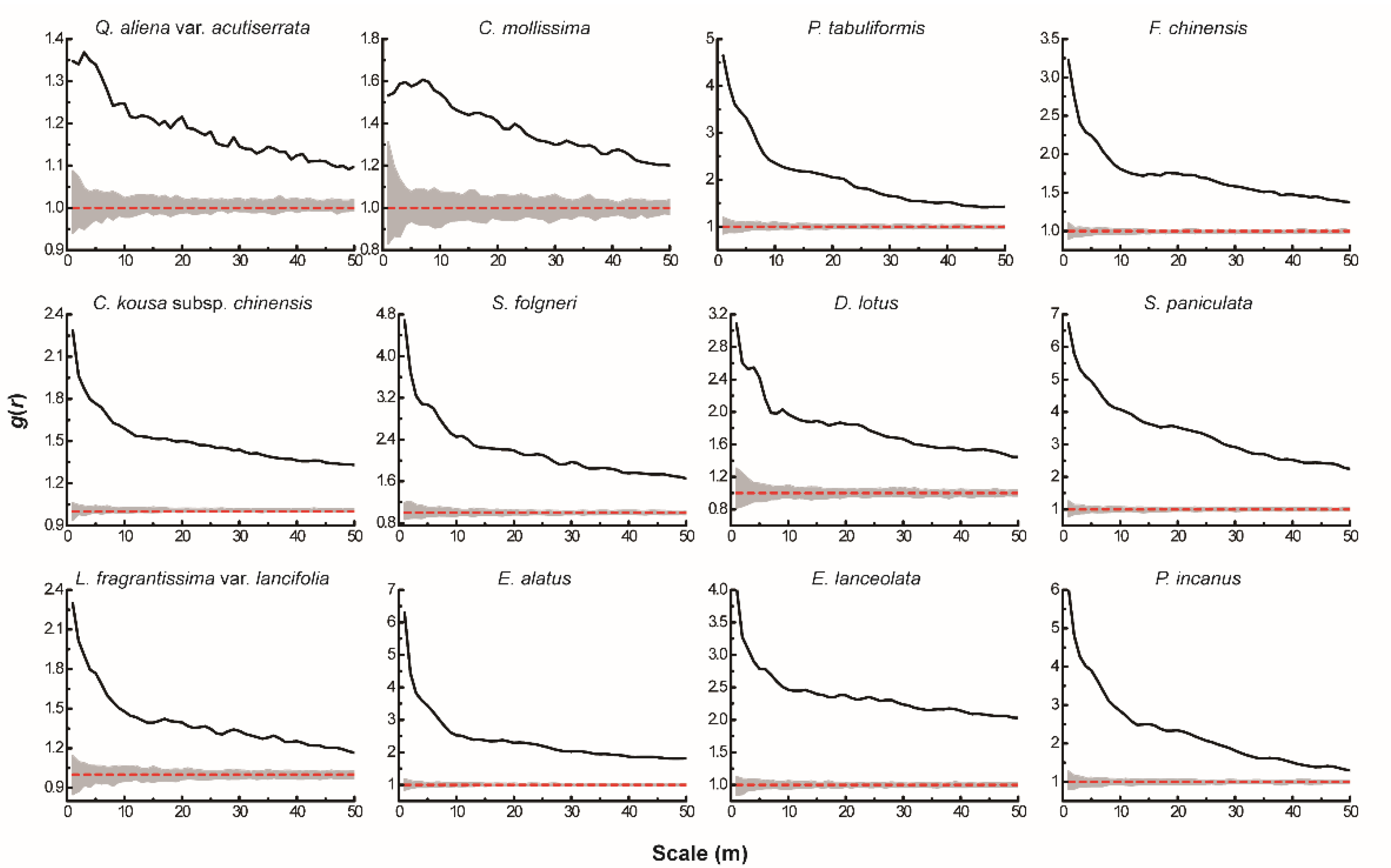
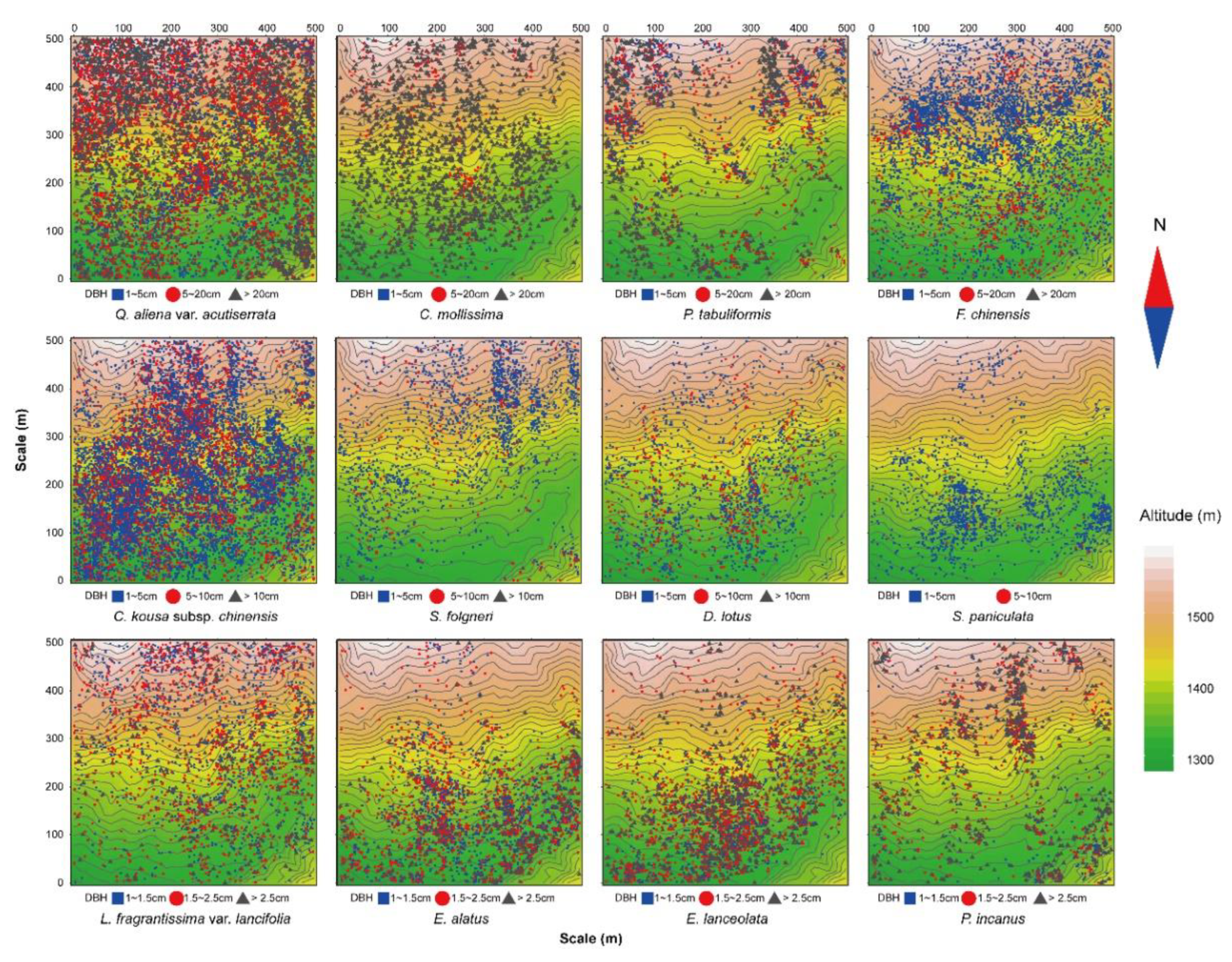
The results of the univariate g(r) function analysis based on the CSR null model (Figure 1) showed that 12 dominant tree species presented a spatial pattern of aggregated distribution throughout the test area, and the degree of aggregation decreased significantly as the scale increased. The actual scattered distribution of each tree species in the plot (Figure 2) was basically consistent with the results of the spatial distribution pattern of tree species under CSR. Thus, without considering other influencing factors, the spatial distribution pattern of each dominant tree species mainly showed aggregated distribution.
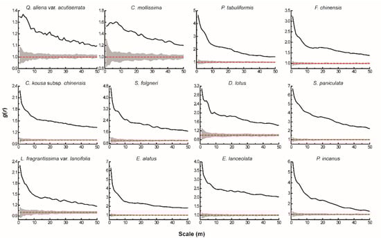
Figure 1.
Spatial distribution pattern of dominant tree species under CSR. The solid black line indicates the observed value of g(r), the red dashed line indicates the theoretical value of g(r). The gray area indicates the 99% confidence interval. The solid black line above the confidence interval indicates aggregation distribution, the solid black line below the confidence interval indicates uniform distribution, and the solid black line between the confidence intervals indicates random distribution.
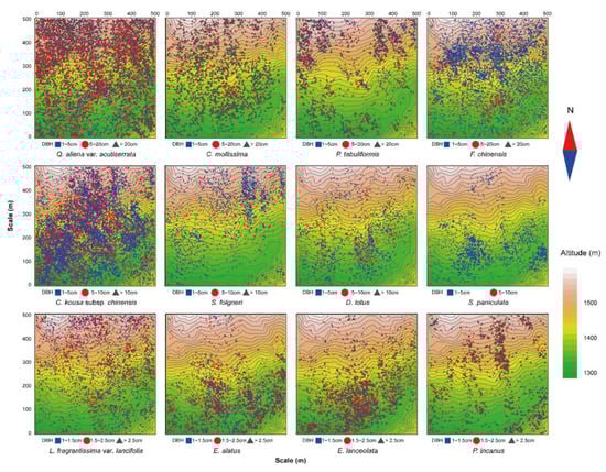
Figure 2.
Spatial distribution map of the 12 dominant tree species.
The HP null model showed significant changes in the distribution pattern of each tree species after eliminating the effect of environmental heterogeneity (Figure 3). Among them, Q. aliena var. acutiserrata Maxim. ex Wenz., P. tabuliformis Carr., 1867 and F. chinensis Roxb. in the tree layer all showed aggregated distribution at scales less than 10 m. As the scale increased, the distribution pattern shifted to random distribution, while C. mollissima Blume showed random distribution throughout the scale after eliminating environmental heterogeneity. C. kousa subsp. Chinensis (Osborn) Q.Y.Xiang, S. folgneri (C.K.Schneid.) Rushforth and D. lotus L. in the sub-arbor layer exhibited aggregated distribution at scales less than 5 m, while S. paniculata Miq. remained aggregated at all scales. All four dominant species in the shrub layer showed a clustered distribution at a scale of less than 10 m.
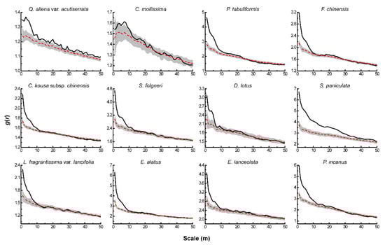
Figure 3.
Spatial distribution pattern of dominant tree species under HP.
3.2. Intra- and Interspecific Associations
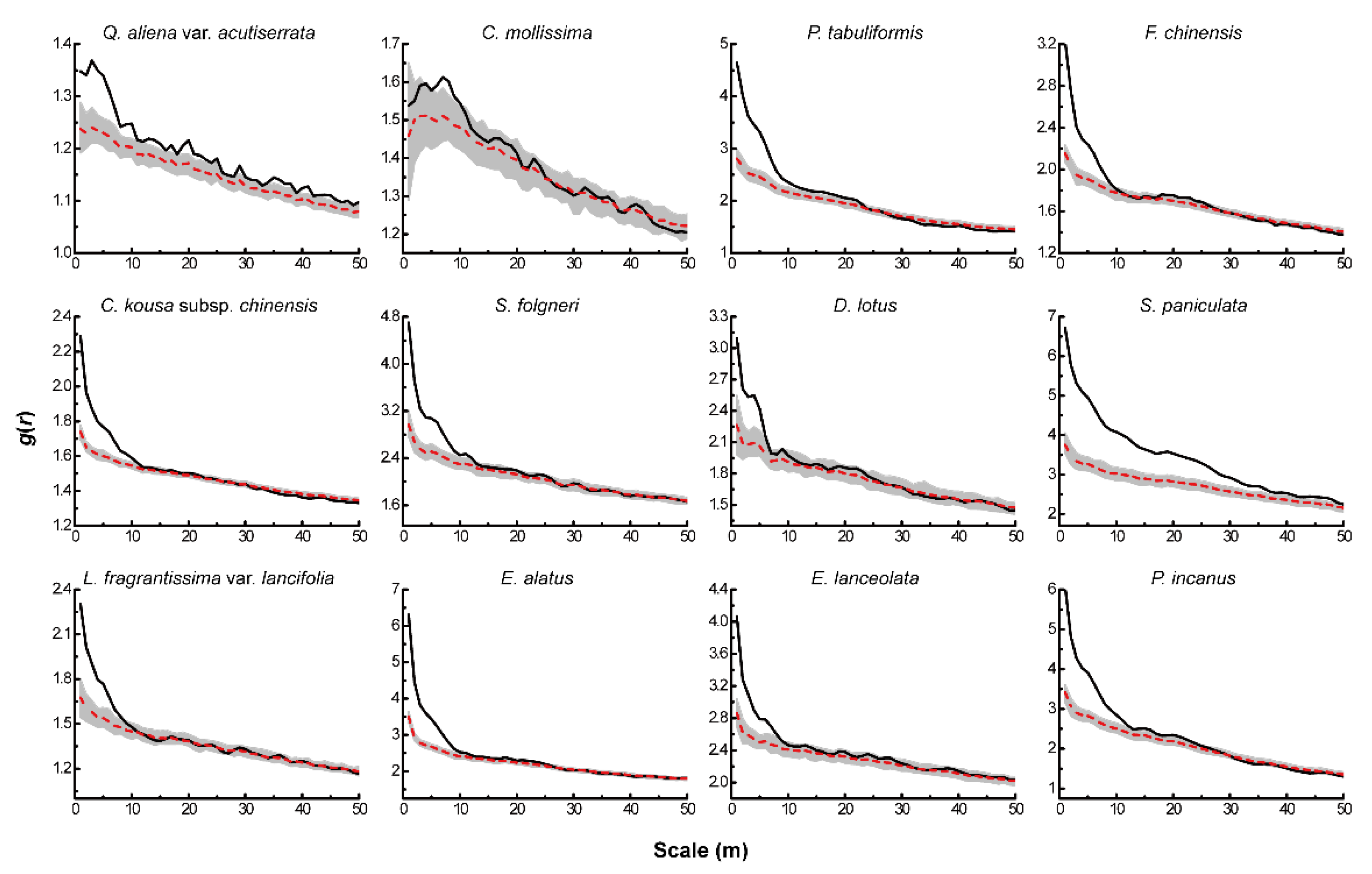
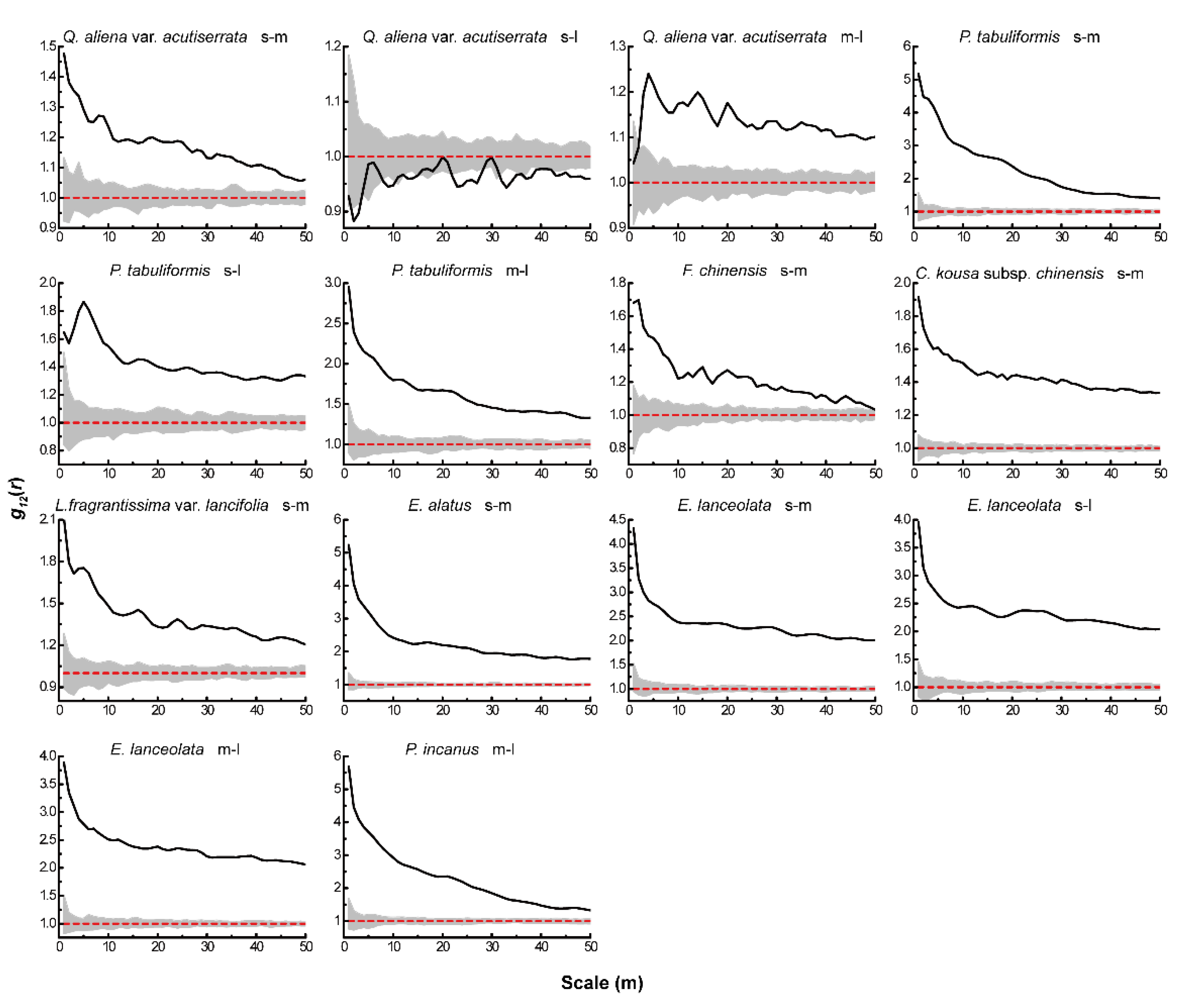
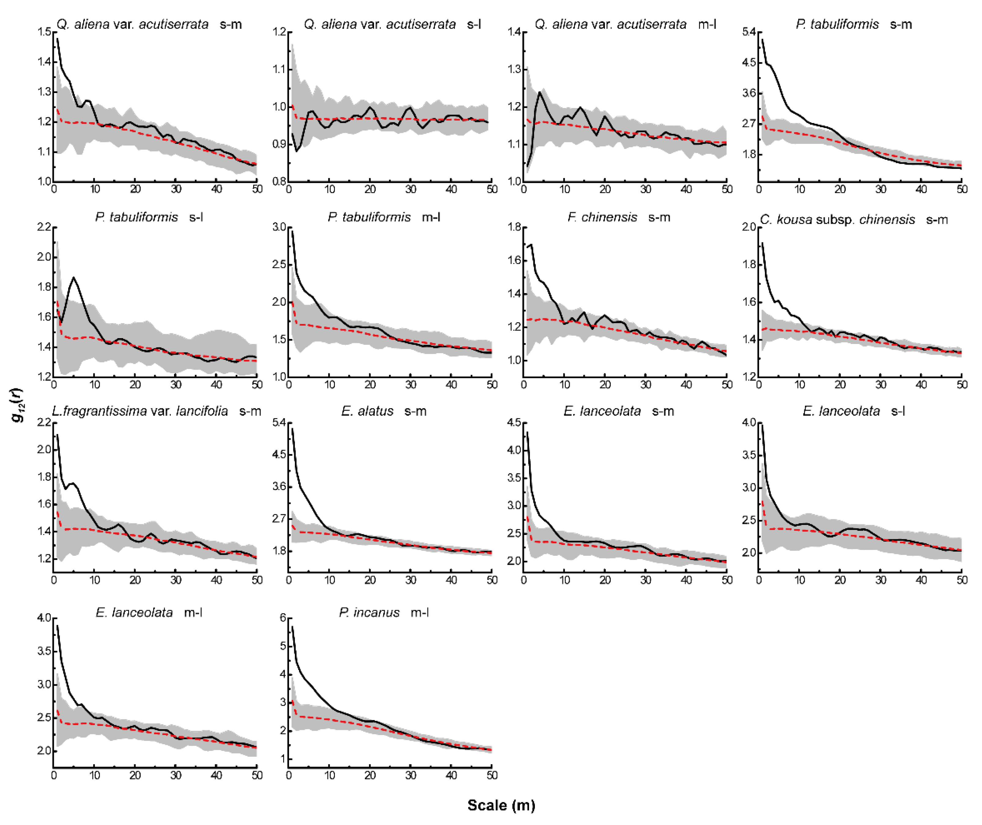
Based on the null models of CSR and AC, we analyzed the associations between different life-history stages of the same tree species. Under CSR (Figure 4), the four dominant species of the tree layer showed positive associations between different life-history stages of all tree species, except for a significant negative association between small and large trees of Q. aliena var. acutiserrata at all scales. There were also significant positive associations between different life-history stages of the dominant tree species in both the sub-arbor and shrub layers across the scales. After eliminating the effect of environmental heterogeneity, the results of the AC null model analysis (Figure 5) showed no significant associations between small and large or medium and large trees in the tree layer of Q. aliena var. acutiserrata at any scale. Different life-history stages of P. tabuliformis and Fraxinus chinensis showed positive associations at the small scale, which shifted to non-significant associations as the scale increased. Small and medium trees in the sub-arbor layer of C. kousa subsp. chinensis showed positive associations between one another only at scales of less than 10 m. The different life-history stages of the dominant tree species in the shrub layer showed positive correlations at small scales, except for the small and large trees of Elaeagnus lanceolata, which showed no significant correlation at any scale.
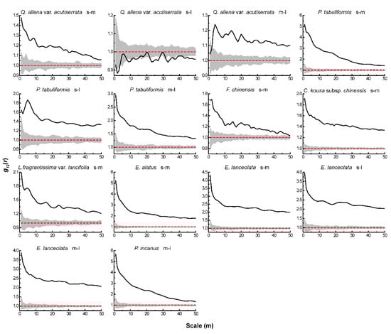
Figure 4.
Intraspecific associations of dominant tree species under CSR. The solid black line indicates the observed value of g12(r), the red dashed line indicates the theoretical value of g12(r). The gray area indicates the 99% confidence interval. The solid black line above the confidence interval indicates a positive association, the solid black line below the confidence interval indicates a negative association, and the solid black line between the confidence intervals indicates no association.
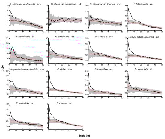
Figure 5.
Intraspecific associations of dominant tree species under AC.
Since large trees in the tree layer were overwhelmingly dominant in height, only the associations between large trees in the tree layer and small trees in the sub-arbor layer and shrub layer were considered in the analysis of the associations between different tree species. Under CSR, among the 21 species pairs analyzed, 12 were significantly negatively associated with each other, while 9 were significantly positively associated with each other (Table 3). Large trees of Q. aliena var. acutiserrata were significantly positively associated with small trees of S. folgneri, though they were not significantly associated with small trees of L. fragrantissima var. lancifolia Rehd. at small scales. They became significantly positively associated with small trees of L. fragrantissima var. lancifolia at scales of more than 10 m, and at these scales, held mainly negative associations with small trees of other species. There were no significant associations between the large trees of C. mollissima and the small trees of S. folgneri at scales of less than 5 m. Significant negative associations emerged at scales of more than 5 m, and mainly positive associations with the small trees of other species. Large trees of P. tabuliformis were significantly positively associated with S. folgneri at all scales. At scales of less than 5 m, they were not significantly associated with small trees of Diospyros lotus, and at scales of more than 5 m, they were significantly negatively associated with small trees of other species.
Table 3.
Species association under CSR at different scales.
However, the results of the analysis under the AC (Table 4) showed that the associations between tree species all changed significantly at large scales after excluding the effect of environmental heterogeneity, mainly showing a lack of significant associations. Associations between large trees of Q. aliena var. acutiserrata and small trees of different species differed at small scales. Large trees of C. mollissima and small trees of different species were mainly non-associated at all scales. The large trees of P. tabuliformis showed a significant negative association only with small trees of S. paniculata in the shrub layer, and showed few significant associations with the small trees of other dominant species. These results indicate that the association between large trees of dominant species in the tree layer and small trees of other species is significantly influenced by environmental heterogeneity.
Table 4.
Species association under AC at different scales.
3.3. Topographic Effects on Spatial Distribution
In this plot, the elevation varied between 1292.7 and 1576.8 m above sea level, the slope varied between 3.1° and 47.4°, and the convexity varied between −9.2 and 19.3. According to the results of Berman’s test (Table 5), elevation was positively associated with dominant species in the tree layer, negatively associated with C. kousa subsp. chinensis, D. lotus, and S. paniculata in the sub-arbor layer, positively associated with Sorbus folgneri, L. fragrantissima var. lancifolia, and P. incanus Koehne in the shrub layer, and negatively associated with E. alatus (Thunb.) Siebold and E. lanceolata Warb., but the associations between elevation and dominant species were not significant. Slope was significantly positively associated with Q. aliena var. acutiserrata, P. tabuliformis, and F. chinensis in the tree layer, significantly positively associated with S. folgneri in the sub-arbor layer, and in the shrub layer, negatively associated with S. paniculata, as well as significantly negatively associated with E. alatus and E. lanceolata. Convexity was significantly positively associated with Q. aliena var. acutiserrata and P. tabuliformis, while it was significantly negatively associated with Fraxinus chinensis, in the tree layer. Moreover, it was significantly negatively associated with C. kousa subsp. chinensis, D. lotus, and S. paniculata, and significantly positively associated with S. folgneri, in the sub-arbor layer, while it was significantly negatively associated with all four dominant species in the shrub layer.
Table 5.
Berman’s test between species and topographical variables based on the assumption of CSR.
4. Discussion
4.1. Spatial Distribution and Species Associations
The spatial distribution patterns of populations are governed by a variety of factors. Generally, they are influenced by species’ biological characteristics at small scales, such as seed dispersal limitations and intra- and interspecific competition, and influenced by environmental heterogeneity at larger scales [42,43]. Environmental gradients are often related to topographic features, such as elevation, slope, and convexity [38,40], which indirectly affect the spatial distribution of soil moisture and nutrients, and thus the spatial distribution of species [44,45]. In general, at a given range, species show aggregated distributions even late in life or at large scales, which can be explained by environmental heterogeneity. After eliminating environmental effects, species still aggregate at different scales, which can be explained by dispersal limitation [46]. In this study, the 12 dominant tree species showed aggregated distribution patterns as the scale increased under CSR. After eliminating environmental heterogeneity, the results of the analysis based on HP showed that 10 dominant tree species showed aggregated distribution patterns at small scales, and we propose that dispersal limitation could have produced the initial spatial aggregation of seeds at small scales. It has been demonstrated that in tropical forests, regardless of environmental heterogeneity, dispersal limitation is a key factor affecting the degree of stump clumping [47,48]. Hence, we speculate that the spatial distribution of the dominant tree species observed in the plot was mainly influenced by environmental heterogeneity and seed dispersal limitation.
In general, due to the spatial availability of resources, the same species growing under different environmental conditions may exhibit completely different spatial patterns [49,50]. Previous studies have revealed a scale-dependence between the spatial distribution of plants and different biotic or abiotic factors [9,51,52,53]. In addition, it has been found that the spatial distribution pattern of species in tropical and subtropical forests is the result of a combination of habitat heterogeneity and dispersal limitation [42,54,55]. In a study of intra-species distribution patterns and interspecific associations of tree species in the temperate-subtropical transition zone, Zhou et al. (2019) showed that environmental heterogeneity and dispersal constraints are important factors in maintaining the spatial distribution of aggregations at different life stages [46]. Hubbell noted that aggregation was related to the mode of seed dispersal and that seedling density decreased almost exponentially away from the parent tree [22]. In this study, the number of small trees with C. mollissima was few, and their seeds were dispersed by gravity. The seeds were gnawed, carried, and stored by animals, and since we can also eat the fruits, human collection could have impacted regeneration, which may explain, to some extent, the low number of small C. mollissima trees recorded. Animal-dispersed species tend to take an aggregation pattern [48,56]. In this study, only F. chinensis, among the 12 dominant species, was wind-dispersed, while the other species were mainly gravity- or animal-dispersed (Table 2). We speculate that the aggregation patterns of gravity- or animal-dispersed species in this plot may best reveal the dispersal limitations.
Density dependence is closely related to conspecific aggregation [36]. Hardy et al. (2004) suggested that although habitat heterogeneity affects the distribution of many species, dispersal limitation is also a major factor affecting the degree of conspecific aggregation [47]. Seidler et al. (2006) showed that the degree and size of spatial aggregation of conspecifics related to the mode of seed dispersal [48]. In this study, the seeds of the dominant tree species were mainly gravity or animal dispersal (Table 2) and thus showed a distribution pattern of aggregation around the parent tree. Recent studies on species abundance and interaction strength in ecological networks have shown that the strength of interactions between species is strongly correlated with abundance, i.e., the greater the chance of two species encountering, the stronger their interactions will be [57,58]. In this study, the number of individuals of 12 species accounted for 59.6% of the total number of individuals, with a high probability of encounters between different species.
We found the dominant tree species in the tree layer were all light-demanding plants (Table 2), which had a competitive advantage for light compared to species in the sub-tree and shrub layers. However, the populations of Q. aliena var. acutiserrata, C. mollissima, and P. tabuliformis were poor at regenerating, especially C. mollissima, where the number of small trees was only 2.8% of the total number of individuals (Table 1), which is not conducive to the regeneration and development of this population. In comparison, the populations of S. folgneri, D. lotus, and S. paniculata (mainly shade-tolerant or mid-tolerant species) contained more small trees than medium and large trees. As such, we speculate that light resources may be an important factor limiting the regeneration of dominant tree species in the tree layer. We also infer from the positive association that medium trees have a positive influence on the growth of small trees, and also have a competitive advantage in resources.
4.2. Effects of Topography
A large number of studies have shown that slope affects forest dynamics and the spatial pattern of trees [59,60,61]. In this study, slope had a significant effect on 7 of the 12 dominant tree species (Table 5). However, significant species-habitat associations do not necessarily mean that habitat determines the spatial distribution of species. The differential effects of topography on species distribution were reflected in the relationship between species’ life-history traits and the importance of species-level habitat heterogeneity [16]. Several studies compared whether there is a significant species-habitat association across life stages [54,62]. Although these studies provided qualitative rather than quantitative evidence, they suggested a strong consistency in species-habitat associations across the life stages of trees.
Notably, in this study, slope and convexity showed significant positive associations with both Q. aliena var. acutiserrata and P. tabuliformis, and significant negative associations with S. paniculata, E. alatus, and E. lanceolata, while interspecific associations between Q. aliena var. acutiserrata, P. tabuliformis and S. paniculata, E. alatus, E. lanceolata were negative. Robert et al. (2003) showed that slope differentially affects tree size, with smaller trees growing lower on steep slopes and larger trees growing significantly higher [61]. This may explain the phenomenon where slope and convexity are mainly positively associated with tree species in the tree layer and negatively associated with tree species in the sub-arbor and shrub layers. Lan et al. (2011) found that elevation was the most important topographic variable affecting species distribution patterns relative to convexity, slope, and aspect [63]. Yet, no significant correlation of elevation with species distribution was found in this study. Instead, convexity had a significant negative correlation with the distribution of 7 of the 12 major dominant species. On concave slopes, a low tree density, small basal area, and unstable surfaces may limit the distribution of species [64].
5. Conclusions
This study focused on the spatial distribution patterns and intra- and interspecific associations of dominant tree species in a Huangguan plot of the Qinling Mountains, China. We can conclude that: (a) the 12 dominant tree species showed an aggregated distribution at small scales, and as the scale increased, the degree of aggregation diminished and shifted to a random or uniform distribution. The spatial distribution of dominant tree species was mainly influenced by environmental heterogeneity. The observed aggregation distribution pattern could indicate dispersal limitation in this plot. (b) The intra-species associations were mainly positive, indicating that the populations regenerated well. Yet, the large and small trees of Q. aliena var. acutiserrata showed negative associations, and we speculate that the small trees are limited by light resources during their growth. In addition, interspecific associations were mainly influenced by the biological characteristics of each species and environmental heterogeneity. (c) The distribution of tree species was significantly influenced by topographic factors, mainly by slope and convexity. Analysis of spatial distribution patterns is the first step to understanding the plant community structure and revealing mechanisms of species’ coexistence, which are influenced by numerous factors: soil heterogeneity, habitat filtering, dispersal limitation, etc. The intensity of the influence of different factors on species’ coexistence requires further investigation and research.
Author Contributions
Q.Y. and Z.H. provided research ideas; C.H., Q.Y., S.J. and Y.L. participated in fieldwork and collected the data; C.H. performed data analysis; C.H. and Q.Y. wrote the manuscript; Q.Y., S.J. and Z.H. revised the manuscript. All authors have read and agreed to the published version of the manuscript.
Funding
This study was financially supported by the National Natural Science Foundation of China (32001171, 32001120) and the China Postdoctoral Science Foundation (2020M680158).
Institutional Review Board Statement
Not applicable.
Informed Consent Statement
Not applicable.
Data Availability Statement
Not applicable.
Conflicts of Interest
The authors declare no conflict of interest.
References
- Gadow, K.V.; Zhang, C.Y.; Wehenkel, C.; Pommerening, A.; Corral-Ravis, J.; Korol, M.; Myklush, S.; Hui, G.Y.; Zhao, X.H. Forest structure and diversity. In Continuous Cover Forestry. Managing Forest Ecosystems; Pukkala, T., von Gadow, K., Eds.; Springer: Dordrecht, The Netherlands, 2012. [Google Scholar]
- Janik, D.; Kral, K.; Adam, D.; Hort, L.; Samonil, P.; Unar, P.; Vrska, T.; McMahon, S. Tree spatial patterns of Fagus sylvatica expansion over 37 years. For. Ecol. Manag. 2016, 375, 134–145. [Google Scholar] [CrossRef] [Green Version]
- Zhang, L.Y.; Dong, L.B.; Liu, Q.; Liu, Z.G. Spatial patterns and interspecific associations during natural regeneration in three types of secondary forest in the central part of the Greater Khingan mountains, Heilongjiang province, China. Forests 2020, 11, 152. [Google Scholar] [CrossRef] [Green Version]
- Purves, D.W.; Law, R. Fine-scale spatial structure in a grassland community: Quantifying the plant’s-eye view. J. Ecol. 2002, 90, 121–129. [Google Scholar] [CrossRef]
- Mokany, K.; Ash, J.; Roxburgh, S. Effects of spatial aggregation on competition, complementarity and resource use. Austral Ecol. 2008, 33, 261–270. [Google Scholar] [CrossRef]
- Detto, M.; Muller-Landau, H.C. Stabilization of species coexistence in spatial models through the aggregation-segregation effect generated by local dispersal and nonspecific local interactions. Theor. Popul. Biol. 2016, 112, 97–108. [Google Scholar] [CrossRef] [PubMed] [Green Version]
- Wiegand, T.; Wang, X.G.; Anderson-Teixeira, K.J.; Bourg, N.A.; Cao, M.; Ci, X.Q.; Davies, S.J.; Hao, Z.Q.; Howe, R.W.; Kress, W.J.; et al. Consequences of spatial patterns for coexistence in species-rich plant communities. Nat. Ecol. Evol. 2021, 5, 965–973. [Google Scholar] [CrossRef] [PubMed]
- Yuan, Z.; Gazol, A.; Wang, X.; Xing, D.; Lin, F.; Bai, X.; Zhao, Y.; Li, B.; Hao, Z. What happens below the canopy? Direct and indirect influences of the dominant species on forest vertical layers. Oikos 2012, 121, 1145–1153. [Google Scholar] [CrossRef]
- Hao, Z.Q.; Zhang, J.; Song, B.; Ye, J.; Li, B.H. Vertical structure and spatial associations of dominant tree species in an old-growth temperate forest. For. Ecol. Manag. 2007, 252, 1–11. [Google Scholar] [CrossRef]
- Ward, J.S.; Parker, G.R.; Ferrandino, F.J. Long-term spatial dynamics in an old-growth deciduous forest. For. Ecol. Manag. 1996, 83, 189–202. [Google Scholar] [CrossRef]
- Jang, W.; Keyes, C.R.; Lim, J.H. Application of mathematical models in the spatial analysis of early tree seedling distribution patterns within a treefall gap at Gwangneung experimental forest, Korea. J. Plant Biol. 2013, 56, 283–289. [Google Scholar] [CrossRef]
- Lutz, J.A.; Larson, A.J.; Furniss, T.J.; Donato, D.C.; Freund, J.A.; Swanson, M.E.; Bible, K.J.; Chen, J.Q.; Franklin, J.F. Spatially nonrandom tree mortality and ingrowth maintain equilibrium pattern in an old-growth Pseudotsuga-Tsuga forest. Ecology 2014, 95, 2047–2054. [Google Scholar] [CrossRef] [PubMed] [Green Version]
- Clark, D.B.; Palmer, M.W.; Clark, D.A. Edaphic factors and the landscape-scale distributions of tropical rain forest trees. Ecology 1999, 80, 2662–2675. [Google Scholar] [CrossRef]
- Baldeck, C.A.; Harms, K.E.; Yavitt, J.B.; John, R.; Turner, B.L.; Valencia, R.; Navarrete, H.; Bunyavejchewin, S.; Kiratiprayoon, S.; Yaacob, A.; et al. Habitat filtering across tree life stages in tropical forest communities. Proc. R. Soc. B Biol. Sci. 2013, 280, 20130548. [Google Scholar] [CrossRef] [PubMed] [Green Version]
- Ye, J.; Hao, Z.Q.; Xie, P.; Li, J.G. Habitat associations of saplings and adults in an old-growth temperate forest in the Changbai mountains, northeastern China. For. Stud. China 2011, 13, 13–22. [Google Scholar] [CrossRef]
- Shen, G.C.; He, F.L.; Waagepetersen, R.; Sun, I.F.; Hao, Z.Q.; Chen, Z.S.; Yu, M.J. Quantifying effects of habitat heterogeneity and other clustering processes on spatial distributions of tree species. Ecology 2013, 94, 2436–2443. [Google Scholar] [CrossRef]
- Zhang, Y.T.; Li, J.M.; Chang, S.L.; Li, X.; Lu, J.J. Spatial distribution pattern of Picea schrenkiana population in the Middle Tianshan Mountains and the relationship with topographic attributes. J. Arid. Land 2012, 4, 457–468. [Google Scholar] [CrossRef] [Green Version]
- Chisholm, R.A.; Condit, R.; Abd Rahman, K.; Baker, P.J.; Bunyavejchewin, S.; Chen, Y.Y.; Chuyong, G.; Dattaraja, H.S.; Davies, S.; Ewango, C.E.N.; et al. Temporal variability of forest communities: Empirical estimates of population change in 4000 tree species. Ecol. Lett. 2014, 17, 855–865. [Google Scholar] [CrossRef]
- Kalyuzhny, M.; Kadmon, R.; Shnerb, N.M. A neutral theory with environmental stochasticity explains static and dynamic properties of ecological communities. Ecol. Lett. 2015, 18, 572–580. [Google Scholar] [CrossRef]
- Stein, A.; Gerstner, K.; Kreft, H. Environmental heterogeneity as a universal driver of species richness across taxa, biomes and spatial scales. Ecol. Lett. 2014, 17, 866–880. [Google Scholar] [CrossRef]
- Lin, G.J.; Stralberg, D.; Gong, G.Q.; Huang, Z.L.; Ye, W.H.; Wu, L.F. Separating the effects of environment and space on tree species distribution: From population to community. PLoS ONE 2013, 8, e56171. [Google Scholar] [CrossRef] [Green Version]
- Hubbell, S.P. Tree dispersion, abundance, and diversity in a tropical dry forest: That tropical trees are clumped, not spaced, alters conceptions of the organization and dynamics. Science 1979, 203, 1299–1309. [Google Scholar] [CrossRef] [PubMed] [Green Version]
- Liu, Y.Y.; Li, F.R.; Jin, G.Z. Spatial patterns and associations of four species in an old-growth temperate forest. J. Plant Interact. 2014, 9, 745–753. [Google Scholar] [CrossRef]
- Nguyen, H.H.; Uria-Diez, J.; Wiegand, K. Spatial distribution and association patterns in a tropical evergreen broad-leaved forest of north-central Vietnam. J. Veg. Sci. 2016, 27, 318–327. [Google Scholar] [CrossRef]
- Peters, H.A. Neighbour-regulated mortality: The influence of positive and negative density dependence on tree populations in species-rich tropical forests. Ecol. Lett. 2003, 6, 757–765. [Google Scholar] [CrossRef] [Green Version]
- Pacala, S.W.; Levin, S.A. Biologically Generated Spatial Pattern and the Coexistence of Competing Species. Monogr. Popul. Biol. 1996, 30, 204–232. [Google Scholar]
- Chai, Z.Z.; Wang, D.X. Environmental influences on the successful regeneration of pine-oak mixed forests in the Qinling Mountains, China. Scand. J. For. Res. 2016, 31, 368–381. [Google Scholar] [CrossRef]
- He, C.M.; Liu, R.Q.; Yang, Z.C.; Yin, Q.L.; Jia, S.H.; Luo, Y.; Hao, Z.Q. Species composition and community structure of warm temperate deciduous broadleaved forests in Huangguan of Qinling Mountains, China. Chin. J. Appl. Ecol. 2021, 32, 2737–2744. [Google Scholar]
- Linares-Palomino, R.; Alvarez, S.I.P. Tree community patterns in seasonally dry tropical forests in the Cerros de Amotape Cordillera, Tumbes, Peru. For. Ecol. Manag. 2005, 209, 261–272. [Google Scholar] [CrossRef]
- Obiang, N.L.E.; Kenfack, D.; Picard, N.; Lutz, J.A.; Bissiengou, P.; Memiaghe, H.R.; Alonso, A. Determinants of spatial patterns of canopy tree species in a tropical evergreen forest in Gabon. J. Veg. Sci. 2019, 30, 929–939. [Google Scholar] [CrossRef]
- Perea, A.J.; Wiegand, T.; Garrido, J.L.; Rey, P.J.; Alcantara, J.M. Legacy effects of seed dispersal mechanisms shape the spatial interaction network of plant species in Mediterranean forests. J. Ecol. 2021, 109, 3670–3684. [Google Scholar] [CrossRef]
- Cressie, N. Statistics for Spatial Data; John Wiley & Sons: Hoboken, NJ, USA, 2015. [Google Scholar]
- Jalilian, A.; Guan, Y.T.; Waagepetersen, R. Decomposition of variance for spatial cox processes. Scand. J. Stat. 2013, 40, 119–137. [Google Scholar] [CrossRef] [PubMed] [Green Version]
- Luo, Z.; Mi, X.; Chen, X.; Ye, Z.; Ding, B. Density dependence is not very prevalent in a heterogeneous subtropical forest. Oikos 2012, 121, 1239–1250. [Google Scholar] [CrossRef]
- Wiegand, T.; Gunatilleke, S.; Gunatilleke, N. Species associations in a heterogeneous Sri lankan dipterocarp forest. Am. Nat. 2007, 170, E77. [Google Scholar] [CrossRef] [PubMed] [Green Version]
- Yan, Z.; Mi, X.; Ren, H.; Ma, K. Density dependence is prevalent in a heterogeneous subtropical forest. Oikos 2010, 119, 109–119. [Google Scholar]
- Wiegand, T.; Moloney, K.A. Rings, circles, and null-models for point pattern analysis in ecology. Oikos 2004, 104, 209–229. [Google Scholar] [CrossRef]
- Gunatilleke, C.V.S.; Gunatilleke, I.; Esufali, S.; Harms, K.E.; Ashton, P.M.S.; Burslem, D.; Ashton, P.S. Species-habitat associations in a Sri Lankan dipterocarp forest. J. Trop. Ecol. 2006, 22, 371–384. [Google Scholar] [CrossRef] [Green Version]
- Harms, K.E.; Condit, R.; Hubbell, S.P.; Foster, R.B. Habitat associations of trees and shrubs in a 50-ha neotropical forest plot. J. Ecol. 2001, 89, 947–959. [Google Scholar] [CrossRef]
- Valencia, R.; Foster, R.B.; Villa, G.; Condit, R.; Svenning, J.C.; Hernandez, C.; Romoleroux, K.; Losos, E.; Magard, E.; Balslev, H. Tree species distributions and local habitat variation in the Amazon: Large forest plot in eastern Ecuador. J. Ecol. 2004, 92, 214–229. [Google Scholar] [CrossRef]
- Berman, M. Testing for spatial association between a point process and another stochastic-process. J. R. Stat. Soc. Ser. C Appl. Stat. 1986, 35, 54–62. [Google Scholar] [CrossRef]
- Lin, Y.C.; Chang, L.W.; Yang, K.C.; Wang, H.H.; Sun, I.F. Point patterns of tree distribution determined by habitat heterogeneity and dispersal limitation. Oecologia 2011, 165, 175–184. [Google Scholar] [CrossRef]
- Kang, D.; Guo, Y.X.; Ren, C.J.; Zhao, F.Z.; Feng, Y.Z.; Han, X.H.; Yang, G.H. Population structure and spatial pattern of main tree species in secondary Betula platyphylla forest in Ziwuling mountains, China. Sci. Rep. 2014, 4, 6873. [Google Scholar] [CrossRef] [PubMed] [Green Version]
- Zuleta, D.; Russo, S.E.; Barona, A.; Barreto-Silva, J.S.; Cardenas, D.; Castano, N.; Davies, S.J.; Detto, M.; Sua, S.; Turner, B.L.; et al. Importance of topography for tree species habitat distributions in a terra firme forest in the Colombian Amazon. Plant Soil 2020, 450, 133–149. [Google Scholar] [CrossRef]
- Costa, F.R.C.; Magnusson, W.E.; Luizao, R.C. Mesoscale distribution patterns of Amazonian understorey herbs in relation to topography, soil and watersheds. J. Ecol. 2005, 93, 863–878. [Google Scholar] [CrossRef]
- Zhou, Q.; Shi, H.; Shu, X.; Xie, F.L.; Zhang, K.R.; Zhang, Q.F.; Dang, H.S. Spatial distribution and interspecific associations in a deciduous broad-leaved forest in north-central China. J. Veg. Sci. 2019, 30, 1153–1163. [Google Scholar] [CrossRef]
- Hardy, O.J.; Sonke, B. Spatial pattern analysis of tree species distribution in a tropical rain forest of Cameroon: Assessing the role of limited dispersal and niche differentiation. For. Ecol. Manag. 2004, 197, 191–202. [Google Scholar] [CrossRef]
- Seidler, T.G.; Plotkin, J.B. Seed dispersal and spatial pattern in tropical trees. PLoS Biol. 2006, 4, 2132–2137. [Google Scholar] [CrossRef] [PubMed]
- Kerns, B.K.; Moore, M.A.; Timpson, M.E.; Hart, S.C. Soil properties associated with vegetation patches in a Pinus ponderosa-bunchgrass mosaic. West. N. Am. Nat. 2003, 63, 452–462. [Google Scholar]
- Law, R.; Illian, J.; Burslem, D.; Gratzer, G.; Gunatilleke, C.V.S.; Gunatilleke, I. Ecological information from spatial patterns of plants: Insights from point process theory. J. Ecol. 2009, 97, 616–628. [Google Scholar] [CrossRef]
- Benot, M.L.; Bittebiere, A.K.; Ernoult, A.; Clement, B.; Mony, C. Fine-scale spatial patterns in grassland communities depend on species clonal dispersal ability and interactions with neighbours. J. Ecol. 2013, 101, 626–636. [Google Scholar] [CrossRef]
- Zhang, J.; Hao, Z.Q.; Song, B.; Li, B.H.; Wang, X.G.; Ye, J. Fine-scale species co-occurrence patterns in an old-growth temperate forest. For. Ecol. Manag. 2009, 257, 2115–2120. [Google Scholar] [CrossRef]
- Hou, J.H.; Mi, X.C.; Liu, C.R.; Ma, K.P. Spatial patterns and associations in a Quercus-Betula forest in northern China. J. Veg. Sci. 2004, 15, 407–414. [Google Scholar]
- Comita, L.S.; Condit, R.; Hubbell, S.P. Developmental changes in habitat associations of tropical trees. J. Ecol. 2007, 95, 482–492. [Google Scholar] [CrossRef]
- May, F.; Huth, A.; Wiegand, T. Moving beyond abundance distributions: Neutral theory and spatial patterns in a tropical forest. Proc. R. Soc. B-Biol. Sci. 2015, 282, 20141657. [Google Scholar] [CrossRef] [PubMed]
- Condit, R.; Ashton, P.S.; Baker, P.; Bunyavejchewin, S.; Gunatilleke, S.; Gunatilleke, N.; Hubbell, S.P.; Foster, R.B.; Itoh, A.; LaFrankie, J.V.; et al. Spatial patterns in the distribution of tropical tree species. Science 2000, 288, 1414–1418. [Google Scholar] [CrossRef] [PubMed]
- Vazquez, D.P.; Melian, C.J.; Williams, N.M.; Bluthgen, N.; Krasnov, B.R.; Poulin, R. Species abundance and asymmetric interaction strength in ecological networks. Oikos 2007, 116, 1120–1127. [Google Scholar] [CrossRef]
- Wang, X.G.; Wiegand, T.; Hao, Z.Q.; Li, B.H.; Ye, J.; Lin, F. Species associations in an old-growth temperate forest in north-eastern China. J. Ecol. 2010, 98, 674–686. [Google Scholar] [CrossRef]
- Baldeck, C.A.; Harms, K.E.; Yavitt, J.B.; John, R.; Turner, B.L.; Valencia, R.; Navarrete, H.; Davies, S.J.; Chuyong, G.B.; Kenfack, D.; et al. Soil resources and topography shape local tree community structure in tropical forests. Proc. R. Soc. B-Biol. Sci. 2013, 280, 20122532. [Google Scholar] [CrossRef]
- Ferry, B.; Morneau, F.; Bontemps, J.D.; Blanc, L.; Freycon, V. Higher treefall rates on slopes and waterlogged soils result in lower stand biomass and productivity in a tropical rain forest. J. Ecol. 2010, 98, 106–116. [Google Scholar] [CrossRef]
- Robert, A.; Moravie, M.A. Topographic variation and stand heterogeneity in a wet evergreen forest of India. J. Trop. Ecol. 2003, 19, 697–707. [Google Scholar] [CrossRef]
- Webb, C.O.; Peart, D.R. Habitat associations of trees and seedlings in a Bornean rain forest. J. Ecol. 2000, 88, 464–478. [Google Scholar] [CrossRef]
- Lan, G.Y.; Hu, Y.H.; Cao, M.; Zhu, H. Topography related spatial distribution of dominant tree species in a tropical seasonal rain forest in China. For. Ecol. Manag. 2011, 262, 1507–1513. [Google Scholar] [CrossRef]
- Enoki, T. Microtopography and distribution of canopy trees in a subtropical evergreen broad-leaved forest in the northern part of Okinawa Island, Japan. Ecol. Res. 2003, 18, 103–113. [Google Scholar] [CrossRef]
Publisher’s Note: MDPI stays neutral with regard to jurisdictional claims in published maps and institutional affiliations. |
© 2022 by the authors. Licensee MDPI, Basel, Switzerland. This article is an open access article distributed under the terms and conditions of the Creative Commons Attribution (CC BY) license (https://creativecommons.org/licenses/by/4.0/).