Mapping China’s Forest Fire Risks with Machine Learning

Abstract

Forest fires are disasters that are common around the world. They pose an ongoing challenge in scientific and forest management. Predicting forest fires improves the levels of forest-fire prevention and risk avoidance. This study aimed to construct a forest risk map for China. We base our map on Visible Infrared Imaging Radiometer Suite data from 17,330 active fires for the period 2012–2019, and combined terrain, meteorology, social economy, vegetation, and other factors closely related to the generation of forest-fire disasters for modeling and predicting forest fires. Four machine learning models for predicting forest fires were compared (i.e., random forest (RF), support vector machine (SVM), multi-layer perceptron (MLP), and gradient-boosting decision tree (GBDT) algorithm), and the RF model was chosen (its accuracy, precision, recall, F1, AUC values were 87.99%, 85.94%, 91.51%, 88.64% and 95.11% respectively). The Chinese seasonal fire zoning map was drawn with the municipal administrative unit as the spatial scale for the first time. The results show evident seasonal and regional differences in the Chinese forest-fire risks; forest-fire risks are relativity high in the spring and winter, but low in fall and summer, and the areas with high regional fire risk are mainly in the provinces of Yunnan (including the cities of Qujing, Lijiang, and Yuxi), Guangdong (including the cities of Shaoguan, Huizhou, and Qingyuan), and Fujian (including the cities of Nanping and Sanming). The major contributions of this study are to (i) provide a framework for large-scale forest-fire risk prediction having a low cost, high precision, and ease of operation, and (ii) improve the understanding of forest-fire risks in China.

1. Introduction

As arguably the most critical land ecosystem, forests maintain ecological balance, conserve soil and water, beautify the environment, trap carbon, and release oxygen [1,2]. However, in recent years, forest ecosystems around the world have come under increasing threat of fires. Forest fires (FFs) are caused by multiple factors, including anthropic activities [3], climate change [4,5], and socio-economic factors [6,7]. They significantly disturb the composition and structure of the environment [8], are among the worst disasters to affect forest ecosystems worldwide, and pose 40 significant threats to the development of modern forestry and human security [9,10,11]. Important tasks for forest ecological management, the provision of early warnings, and risk decision making include (i) simulating and predicting severe occurrence conditions for FFs (such as weather, terrain, and vegetation), (ii) formulating accurate prevention and emergency response strategies to avoid the potential impact of FFs, and (iii) mastering the spatial patterns and rules of FFs (including space, time, and scope) [12,13]. These tasks are helpful for designing fire-management strategies for fire-prevention departments, and effectively planning for and reducing potential fire risks.

Numerous researchers and managers have conducted FF risk-assessment studies, which can be divided into the following three categories. The first category involves studies based on expert knowledge [14,15]. However, this method is subjective because (i) expert knowledge is mostly empirical, (ii) objectively it involves randomness, fuzziness, and inadequacy, and (iii) its accuracy is affected by experience. The second category involves bivariate and multivariate methods, which have been most commonly used in recent years. This category has two subdivisions [16], the first being studies where the possibilities of FFs are assessed using mathematical equations and models, including the Gompit regression model (also known as the complementary log-log model) [17], and geographically weighted regression [18]. However, probabilistic methods have numerous disadvantages and large differences in applicability, meaning that they cannot mine deeper information. The second subdivision comprises studies in which the probabilities of FFs are estimated based on statistics, including evidence theory [19], fence (hurdle) models [20], Poisson regression models [21], and frequency ratios [22]. However, statistical methods are developed based on hypotheses, and the data are analyzed and described from a static perspective assuming that the occurrence conditions of the input FF data remain unchanged and that the past and future are the same; however, in reality, FFs are complex. The third category involves studies using in-depth analysis based on machine learning (ML) and mining of the information in environmental variables for FF prediction. ML methods such as the random forest (RF) algorithm, support vector machines (SVMs), and neural networks (NNs) are used widely in FF prediction modeling, and have shown good results and great potential [23,24].

Since the major FFs in the Greater Hinggan Mountains in Northeast China in 1987, an increasing amount of fire research has been conducted in China. Especially given its strict fire-fighting policy, China is a key area for understanding fire activities. In the history of China, information about FF events—including their location, time, combustion area, casualties, and cause—has been recorded, coordinated, and reported by regional governments at all levels. However, local government agencies report only serious fires, and therefore errors and uncertainties in the process are gradually increasing, and official statistics can only represent the minimum value of the FF area [25]. FFs are affected by factors such as topography, vegetation type, meteorological conditions, fuel, and human activity [26,27]. Assessing large-scale FFs is challenging and complex because of the variety of data sources and the complexity of modeling. A key problem to be solved is how to conduct large-scale FF research combined with ML, multi-source data, and multi-variable factors.

Particularly in China—a large country with great environmental and social variation—exploring the impacts of natural and human factors on the occurrence and distribution of FFs remains a challenge in forest ecological management [28], and the characteristics and drivers of FFs differ across spatiotemporal scales [29]. To date, research on FFs in China has focused mostly on specific provinces or regions, with little national-scale FF research and even less FF risk research in municipal (autonomous prefecture) administrative divisions in large-scale areas. Furthermore, although there have been studies involving classification of FF risk ratings and predicting FFs, these have mostly considered single influencing factors and used relatively few analysis methods. The spatial patterns at a national scale and the spatial distribution characteristics of FFs in municipal (autonomous prefecture) administrative divisions are lacking, and relevant information regarding FF management is scarce. Understanding the factors influencing FFs in China and predicting their development is very important for (i) allocating resources for fire prevention, firefighting, and forest management and (ii) reducing the catastrophic consequences of FFs.

In the present study, we used Visible Infrared Imaging Radiometer Suite (VIIRS) data from 17,330 active Chinese FFs in the period 2012–2019 to predict FFs in China. Specifically, the study included the following steps and achievements. (1) Various factors contributing to FF disasters—such as terrain, climate, and anthropogenic and social factors—were chosen and assimilated. (2) A technical framework for large-scale FF monitoring and prediction with low cost, high accuracy, and high operability was established. Various FF-occurrence prediction models were constructed with the help of an ML algorithm. (3) The best model was then used to map the distribution of FF risks and zoning in China; by analyzing the spatial and temporal distribution characteristics and ignition factors, a refined understanding of FFs in China was obtained (at national, provincial, and municipal levels), thereby reducing the time and costs associated with fire-control work. The present results provide a reference for the Chinese government to optimize investment and resource allocation in FF management and reduce potential risks.

2. Materials and Methods

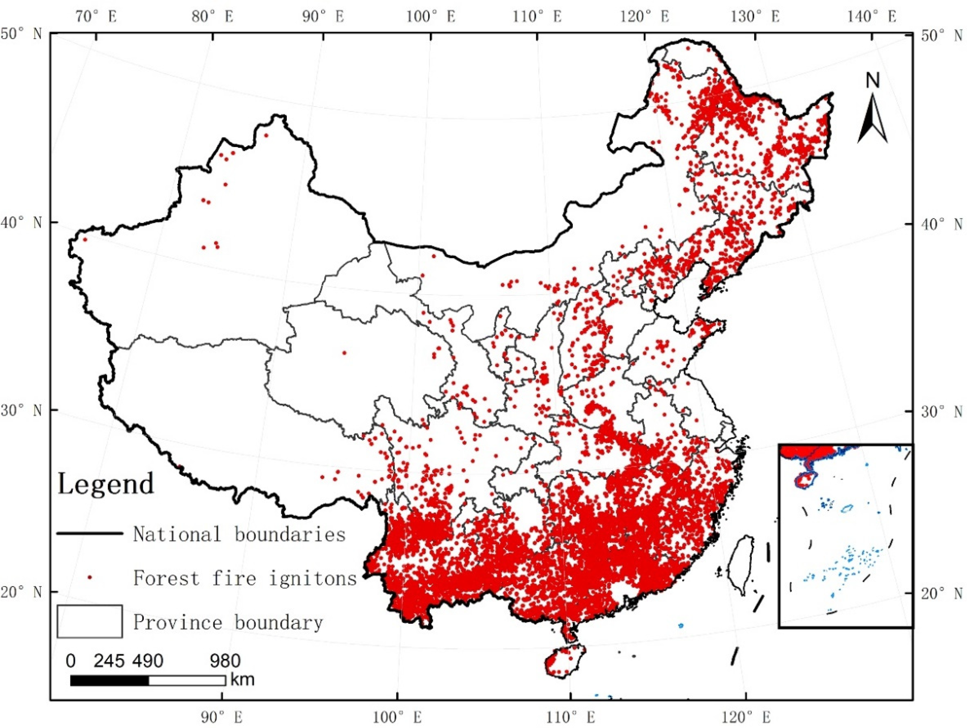
2.1. Study Area

The study area spanned mainland China (Macao, Hong Kong, and Taiwan were not analyzed because of a lack of data). The altitude of the study area is high in the west and low in the east, with diverse topography and landforms. The west is dominated by plateaus, enormous mountains, and deserts; the north is dominated by grasslands and deserts; and the south has hills, mountains, basins, and tropical rainforests [30]. China’s total forest resources are not high, have uneven regional distribution, and are of low quality. Most forests are located in the northeastern, southeastern, and southern parts of China. The climate types are complex, diverse, and substantially different. The population density is large in places: the eastern and southern coastal areas have a high level of economic development and large population density, whereas the western regions have a low level of economic growth and low population density. The occurrence of FFs is affected by climate, terrain, population, economic level, and other factors. China has a vast territory, a complex terrain, a diverse climate, and great regional differences in economic development. China’s FFs show different distribution patterns. The fire product used in the present study uses data from NASA’s Fire Information for Resource Management System (FIRMS). We selected 17,330 fire points within the forest cover. The statistics for fire points in the study area are as follows: there were 1496 fire points in northeast China (Heilongjiang, Jilin, and Liaoning), 2648 in eastern China (Anhui, Shandong, Jiangsu, Zhejiang, Jiangxi, and Fujian, among others), 841 in northern China (Beijing, Tianjin, Inner Mongolia, Hebei, and Shanxi), 3823 in southern China (Guangdong, Guangxi, and Hainan, among others), 2612 in central China (Hebei, Hubei, and Hunan), 219 in northwest China (Gansu, Ningxia, Qinghai, Shaanxi, and Xinjiang), and 5707 in southwest China (Sichuan, Chongqing, Yunnan, Guizhou, and Tibet), as shown in Figure 1.

2.2. Data Sources and Description

2.2.1. Forest-Fire Data Sources and Processing

The VIIRS Active Fire Location vector product source used in the present study comprises data from the NASA Fire Information for Resource Management System (FIRMS) (https://earthdata.nasa.gov/firms). The data contain information about grid center-point location (longitude, latitude), time (year/month/day/hour/minute), brightness (including confidence), and sensors. The VIIRS 375 m thermal anomalies/active fire product provides data from the VIIRS sensor aboard the joint NASA/NOAA Suomi National Polar-orbiting Partnership (Suomi NPP) and NOAA-20 satellites. Based on the Moderate Resolution Imaging Spectroradiometer (MODIS) fire and thermal anomaly algorithm (MOD14/MYD14), the VIIRS active fire product suite systematically draws the global fire activity map at a time interval of ≤12 h [31]; it has a higher spatial resolution (375 m pixels compared to 1 km ones) [31] and replaces the MODIS live fire data in previous global forest observations. This high resolution enables VIIRS to detect fires that Moderate Resolution Imaging Spectroradiometer (MODIS) ignores; fires in relatively small areas provide a greater response and an improved map of the perimeters of large fires, with improved nighttime performance. The VIIRS data are well suited to supporting fire management and improving the fidelity of fire maps [31].

We use high-confidence fire points as the sample points (the high confidence is due to the fire products and does not need to be defined here), and the Chinese land-use dataset provides the range of forestland on the Chinese mainland in 2020 at a spatial resolution of 1000 m with an accuracy of over 93% [32]. From this range, we identified 17,330 high-confidence FF points within the forest coverage of the Chinese mainland in 2012–2019. The forestland coverage was obtained from Data Center for Resources and Environmental Sciences, Chinese Academy of Sciences (https://www.resdc.cn/, accessed on 1 January 2022).

To establish a prediction model for FF occurrence, certain reoccurring FF data are needed, as the dependent variable is set to either occur or not occur [33]. In the present study, we used ArcGIS 10.4 to create a proportion of random points (i.e., points with no ignition are selected in the ratio of 1:1). The dependent variable was set to 1 for fire points and 0 for non-fire points. The selection of sample points follows the double randomness in time and space. The random points were created by the ArcGIS 10.4 software and based on the national land-use data in 2020. The random points in water areas, urban land, and the ocean were eliminated, thereby ensuring that the random points are within the forestland area, resulting in 35,290 random points. Finally, the training set and the test set were divided in a ratio of 7:3.

2.2.2. Other Data

Each factor affects FF occurrence in a unique way, and the selection of factors affects the performance and quality of the FF prediction models. Based on previous studies [34,35,36,37,38,39], numerous analyses, field surveys, and comprehensive consideration of data availability, we finally selected four factors and 20 FF-disaster-causing variables. Dictated by special traditional Chinese customs (including sacrificial fires, holidays, etc.), our study involved special festivals. All of the variables are described in detail in

Table 1. Description of datasets used in the present study.

Sub-Classification	Data	Source	Resolution, Units	References
Topographic	Aspect	https://www.resdc.cn	1 km	[34]
	Slope	https://www.resdc.cn	1 km
	Elevation	https://www.resdc.cn	1 km
Climatic	Daily average ground surface temperature	China Ground Climate Data (V3.0) Daily Dataset,	0.1 °C	[11,35]
	Daily maximum surface temperature	National Meteorological Information Centre	0.1 °C
	Cumulative precipitation from 20–20 h	(https://data.cma.cn, accessed on 1 January 2022)	0.1 mm
	Average air pressure		0.1 hPa
	Daily average relative humidity		1%
	Daily minimum relative humidity		1%
	Sunshine hours		0.1 h
	Mean temperature		0.1 °C
	Daily maximum temperature		0.1 °C
	Average wind speed		0.1 m/s
	Maximum wind speed		0.1 m/s
Vegetation	FVC	https://www.resdc.cn	1 km	[36,37]
Socioeconomic	Road network	https://www.webmap.cn (accessed on 1 January 2022)	1:1,000,000	[38]
	Residential area	https://www.webmap.cn	1:1,000,000
	GDP	https://www.resdc.cn	1 km
	Population	https://www.resdc.cn	1 km
	Special holiday	-	-	-

.

The factors in Table 1 can be divided into five sub-classifications, as follows.

• Topographic

The topography affects the distribution and composition of vegetation and the local and regional microclimate, and is an essential causative factor of FF disasters [39]. The slope affects the combustion speed and direction, the elevation affects the spatial distribution and composition of the forest, and slope direction affects solar radiation, moisture, and forest density. We downloaded Chinese digital elevation data at a 90 m resolution from the Geospatial Data Cloud (https://www.gscloud.cn, accessed on 1 January 2022) to extract terrain-related variables (slope, elevation, and slope direction).

2.

Climatic

Climatic factors such as temperature, rainfall, and wind have a strong influence on FF behavior [11]. Climate variables affect changes in fuel accumulation and water, vegetation distribution, oxygen content in the air, thereby affecting the occurrence and development of FFs. In the present study, we obtained the China Ground Climate Data (V3.0) Daily Dataset from the National Meteorological Information Center (https://data.cma.cn), which includes daily data from 824 national meteorological stations in China. The values of daily climate variables for each fire point and non-fire point were provided by the meteorological station nearest to the point [11].

3.

Vegetation

Vegetation is essential in fire induction, with the fractional vegetation cover (FVC) representing the corresponding amount of fuel for each fire or control point. FVC refers to the percentage of the vertical projection area of the aboveground part of the vegetation on the ground in the total area of the statistical area [37]. We downloaded the normalized difference vegetation index (NDVI) for 2012–2019 from the Resources and Environment Data Center of the Chinese Academy of Sciences (CAS) (https://www.resdc.cn), NDVI time series data based on SPOT/VEGETATION and MODIS satellite remote sensing images, and calculated the FVC from the pixel dichotomy as [37]:

FVC = (NDVI − NDVI_soil)/(NDVI_veg − NDVI_soil),

(1)

where NDVI_soil and NDVI_veg are the selected maximum NDVI and minimum NDVI, respectively, having a confidence of more than 95% [40].

4.

Socioeconomic

Most FFs occurring around the world are highly related to human activity. Socioeconomic variables influence the probability of FFs by affecting human activity. The existence of roads is an essential factor in fire occurrence, and roads have a significant impact on fire ignition [41]. People picnicking, throwing cigarette butts, and/or burning incense near a road may cause a fire. Furthermore, fires may occur at tourist attractions or in densely populated areas, and cigarette butts thrown by people or fire sources left over from sacrifices may cause FFs. As the socioeconomic elements causing fires, we selected settlements, population, GDP (gross domestic product is the final result of the production activities of all permanent residents of a country/region in a certain period), and certain unique festivals (Tomb Sweeping Day, Chinese Halloween, Spring Festival, and the Lantern Festival). In general, these reflect the accessibility of forests and the possibility of people engaging in fire-prone behavior therein. We downloaded the population and GDP data from the Resources and Environment Data Center of the CAS (https://www.resdc.cn) and the road and residential-area data from the National Geographic Information Resource Catalog System (https://www.webmap.cn).

We normalized all the data (climate, terrain, socioeconomic, etc.) to eliminate dimensions, avoid numerical problems due to excessively large values, and balance the contributions of the various factors. We converted all data into numbers between 0 and 1, and the normalization formula was [41]:

$${\mathit{x}}_{\mathit{i}}^{*}=\frac{{\mathit{x}}_{\mathit{i}}-{\mathit{x}}_{\min }}{{\mathit{x}}_{\max }-{\mathit{x}}_{\min }}$$

(2)

where ${\mathit{x}}_{\mathit{i}}$, ${\mathit{x}}_{\mathit{i}}^{*}$, are the values before and after normalization, respectively, and ${\mathit{x}}_{\max }$, ${\mathit{x}}_{\min }$ are expressed as full sample data maximum and minimum, respectively.

2.3. Methods

Figure 2 shows a technical flowchart of the present study. We established a framework for generating FF risk-prediction plots and generated China’s FF risk map with a resolution of 1 km. First, we selected factors related to FF risk and obtained the main drivers of FFs in China. Second, using these factors as input data for the FF prediction models, we applied four commonly used advanced ML models—(i) a multi-layer perceptron (MLP), (ii) an RF, (iii) an SVM, and (iv) a gradient boosting decision tree (GBDT)—to obtain their corresponding results. The accuracy of each model was determined by evaluation indicators (accuracy, precision, recall, f1, and AUC), and the ML models were run using Python 3.8. Third, we selected the best of the four models to predict FF risks in China. Finally, we used ArcGIS 10.4 to carry out kriging interpolation of the annual and seasonal FF risks in China, partition the fire risks, make a thematic map, and evaluate the FF risks.

2.3.1. Random Forest

The RF algorithm was developed by Breiman [42]; it is an ensemble classifier in the form of a nonparametric ML algorithm containing multiple decision trees. To build this model, two parameters are required: (i) the square root of the factor number and (ii) the number of trees running the model. RFs use a randomly selected subset as training samples and variables, and the final classification decision generates the probabilities of various categories by computing all decision trees [42]. The integration method used most commonly for RF is the tensor voting method, and the popularity of this majority voting method is due to its simplicity and effectiveness.

The process for constructing an RF is as follows [43]. Samples are drawn randomly from the original training samples by bootstrap, and training the sample yields a decision tree model. Then, at each node of the decision tree, features are selected randomly to split the node, with no pruning. After repeating the above procedure to generate n decision trees, for each new test sample, the classification results for multiple decision trees are integrated as the classification results for an RF. The final results are obtained by aggregating the outputs of all trees, the formula for which is:

$$\mathit{y}=\frac{1}{\mathit{n}}{\sum }_{\mathit{i}=1}^{\mathit{n}},$$

(3)

where y_i(x) is the predicted output of vector x.

The RF method uses the Gini exponential [44] as a measure of the best split selection to measure impurities in a given element relative to the remaining categories. The formula for the Gini exponential is:

$${\mathit{I}}_{\mathit{T}}\left(\mathit{p}\right)={{\displaystyle \sum }}_{\mathit{i}=1}^{\mathit{j}}{\mathit{p}}_{\mathit{i}}{{\displaystyle \sum }}_{\mathit{k}\ne \mathit{i}}{\mathit{p}}_{\mathit{k}}=1 -{{\displaystyle \sum }}_{\mathit{i}=1}^{\mathit{j}}{\mathit{p}}_{\mathit{i}}^2,$$

(4)

where j indicates the category, T indicates the dataset, and i indicates the label.

The RF classifier has become popular for classification, prediction, and studying variable importance, and can run effectively on large datasets and process high-dimension data. However, some noisy classification or regression problems will be over-stimulated [42,43,44].

In the present study, we tested the effects between 15 and 2000 trees. From comparing the results (accuracy, precision, recall, f1, and AUC), the effect of 35 trees was found to be optimal; thus, we finally selected 35 trees, using the Gini coefficient to measure the impurity.

2.3.2. Support Vector Machine

SVM is a generalized linear classifier that performs binary classification of data using supervised learning methods based on statistical learning theory. It identifies a single boundary between two classes, whose decision boundary is the maximum edge distance hyperplane solved for the learning sample. In particular, SVM separates the training data used by the dataset by determining an optimal (a line in the simplest case). The vector corresponding to the dataset in space cannot be separated by the hyperplane, which is referred to as a linear inseparable. In dealing with this problem, it handles the data from a low-dimension to a high-dimension space, where the projection process depends on the use of appropriate nuclear function [45]. The following kernel functions [46] are commonly used in SVMs:

linear kernel:

$${\mathit{K}(\mathit{x}}_{\mathit{i}}{,\mathit{x}}_{\mathit{j}}{)=<\mathit{x}}_{\mathit{i}}{,\mathit{x}}_{\mathit{j}}>;$$

(5)

polynomial kernel (poly):

$${\mathit{K}(\mathit{x}}_{\mathit{i}}{,\mathit{x}}_{\mathit{j}}{)=(<\mathit{x}}_{\mathit{i}}{,\mathit{x}}_{\mathit{j}}{>+1)}^{\mathit{q}};$$

(6)

radial basis function (RBF):

$${\mathit{K}(\mathit{x}}_{\mathit{i}}{,\mathit{x}}_{\mathit{j}}{)=\mathit{e}}^{-\frac{\Vert {\mathit{x}}_{\mathit{i}}{-\mathit{x}}_{\mathit{j}}{\Vert }^2}{{2\mathsf{\sigma }}^2}}$$

(7)

Optimizing the parameter values of the ML algorithm effectively improves the performance of the model, and RBF and poly are useful for nonlinear hyperplanes [47]. An optimal classification surface is constructed in the feature space based on the theory of structural risk minimization, allowing the model to obtain a global optimum. Because they require few parameters, need only a small number of samples, and have strong generalization ability, SVMs are effective for solving the problems of local convergence, nonlinearity, and overlearning, among others [48]. SVMs can effectively manage small training datasets and often provide high accuracy. However, large-scale training samples are difficult to implement, and it is difficult to solve multi-classification problems, which are sensitive to the selection of parameters and kernel functions [45,46,47,48]. We tested the effects of four kernel functions—polynomial, sigmoid, RBF, and linear—and finally the kernel function was selected in our case.

2.3.3. Multi-Layer Perceptron

MLP is a feed-forward artificial NN model that maps multiple input datasets to a single output dataset. The first layer is the input layer, the last layer is the output layer, and the middle layers are the implied layers [49]. In an MLP, the number of implied layers is not specified and can be chosen according to need. MLPs have good nonlinear mapping capability, high parallelism, and global optimization characteristics, and they are connected by functions consisting of multiple linear and nonlinear activation functions [50,51]. Their disadvantages include (i) difficult selection of the number of hidden nodes of the network, (ii) slow learning speed. In summary, an MLP can be expressed as:

$${\mathit{MLP}=\mathit{Purelin}\left(\mathit{relu}\right(\mathit{W}}_3{ \times \mathit{relu}(\mathit{W}}_2{ \times \mathrm{relu}(\mathit{W}}_1{ \times \mathit{x}}_0{+\mathit{b}}_1{)+\mathit{b}}_2{)+\mathit{b}}_3\left)\right)$$

(8)

where MLP is the MLP model, Purelin is the linear transfer function, relu (rectified linear unit) is the activation function, W corresponds to the weights of the neurons, b corresponds to the biases, and x corresponds to the input data.

The model has good robustness to noise, high fault tolerance, high generalization learning ability, and good application effect. However, the number of hidden nodes in the network is very difficult to select, the learning speed is slow, and the learning may not be sufficient [49,50,51].

The MLP training process is as follows. Using the input features of all samples in the training set as the input layer, the error is obtained by forward propagation. The error then corrects the weight value by back propagation, and finally an optimal model is obtained. The forward and reverse propagations are repeated until the output error is below a set criterion. In the present study, the number of neurons in each hidden layer was 13, the maximum number of iterations was 500, the learning rate was 0.001, and a rectified linear unit (ReLU) activation function was used.

2.3.4. Gradient Boosting Decision Tree

GBDT is an iterative decision-tree algorithm that consists of multiple decision trees. There is a risk of underfitting if there are too few decision trees, and there is a corresponding risk of overfitting with too many. As such, an intermediate number must always be found, whereupon the results of all the trees can be incorporated as the final result [52]. Through multiple rounds of iteration, each round produces a weak classifier. For the same training-set fitting effect, the smaller the learning rate, the more iterations required. Each classifier is trained based on the gradient of the previous game of classifiers. The GBDT core uses the negative gradient of the loss function as the residual approximation in the lifting tree algorithm to minimize the loss function by gradually decreasing the residual values [53]. A single decision tree usually leads to overfitting, and the GBDT model is able to solve this problem by integrating many weak decision trees. This algorithm has high prediction accuracy and strong robustness. Various types of data can be processed flexibly, including both continuous and discrete values, and overfitting can be avoided to some extent. The main advantage of a GBDT lies in its ability to handle dense numerical features effectively. However, it is difficult to adapt to dynamic data generation, and the effect is very poor in the face of sparse classification features [52,53,54,55].

The GBDT model [54] can be expressed as:

$${\mathit{F}}_{\mathit{M}}\left(\mathit{x}\right)={\displaystyle \sum }_{\mathit{m}=1}^{\mathit{M}}{\mathit{T}(\mathit{x};\theta }_{\mathit{m}}),$$

(9)

where T(x; θ_m) corresponds to the decision tree, θ_m corresponds to the parameters of the tree, and M corresponds to the number of trees. The GBDT was determined by minimizing the loss function, and the main flow [55] of this algorithm is as follows. Samples are first extracted from the dataset, and the residuals are calculated for each sample. The residuals are then used as the training data, and the optimal partition nodes are selected by minimizing the loss function. The samples are then redivided and the model is updated, iterating constantly until the mean square error is minimized. The number of weak learners in the present study was 100, with a learning rate of 0.1.

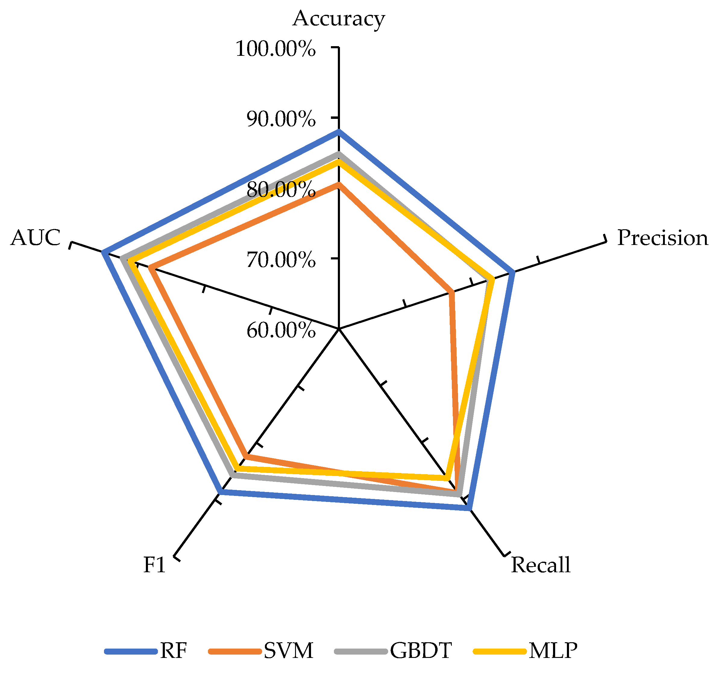
2.3.5. Evaluation of the Performance of the Models

To evaluate the quality of the results, we assessed the model effects using five performance indicators, i.e., accuracy, precision, recall, f1, and area under the curve (AUC) [56,57]. The accuracy is the most commonly used estimator, recall represents the extent to which positive cases are predicted in the sample, precision represents the proportion of accurately predicted positive cases, f1 serves as a measure of the values of precision and recall, and AUC represents the area enclosed by the coordinate axis under the receiver operating characteristic (ROC) curve [56,57]. As a classifier, the best case is both high precision and high recall, but, in reality, it is usually high precision and low recall or low recall and high precision. New approaches are therefore needed to balance the two proportions. The more classical method is F1, and this can be calculated using [56]:

$$\mathit{Accuracy}=(\mathit{TP}+\mathit{TN})/(\mathit{TP}+\mathit{FP}+\mathit{TN}+\mathit{FN}),$$

(10)

$$\mathit{Recall}=\mathit{TP}/(\mathit{TP}+\mathit{FN}),$$

(11)

$$\mathit{Precision}=\left(\mathit{TP}\right)/(\mathit{TP}+\mathit{FP}),$$

(12)

$$\mathit{F}1=2\times (\mathit{Precision} \times \mathit{Recall})/(\mathit{Precision}+\mathit{Recall}).$$

(13)

Here, TP (true positive) is the number of positive samples correctly predicted as positive by the classifier, and FP (false positive) is the number of negative samples incorrectly predicted as positive; similarly, TN (true negative) is the number of negative samples correctly predicted as negative by the classifier, and FN (false negative) is the number of positive samples incorrectly predicted as negative.

In the receiver operating characteristic (ROC) space, the relationships corresponding to TP and FP exhibited by the data are drawn to form the ROC curve. The lowest AUC value represents the measure of the worst separability, whereas the highest AUC value represents the measure of the perfect separability [58]. The AUC result is acceptable at 0.7–0.8, excellent at 0.8–0.9, and exceptional at >0.9. The AUC formula [59] can be expressed as:

$$\mathit{AUC}=\sum \mathit{TP}+\sum \mathit{TN}/(\mathit{P}+\mathit{N}).$$

(14)

3. Results

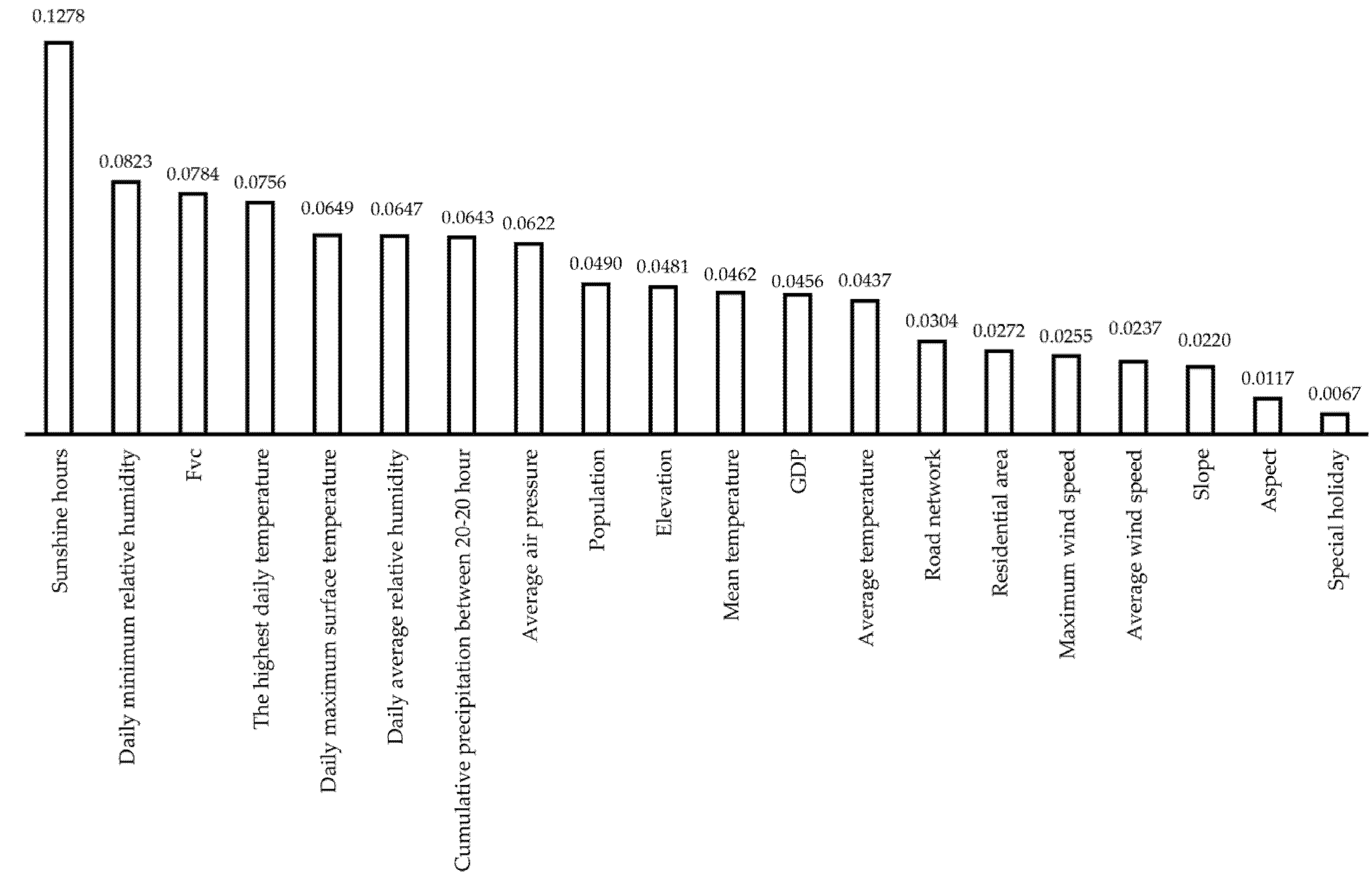
3.1. Model Comparison and Validation

As described previously, 30% of the test data were not used to train the model, and these were treated as the validation data. Therefore, the results were compared to the validation data. We validated the performance of the four ML models using their accuracy, recall, F1 values, and AUC evaluation metrics. Based on validation dataset test results (shown in Figure 3), the results from all four models were considered acceptable in appearance (AUC ≥ 0.8). A higher precision value indicates that a model has good prediction for positive samples, and the order of the precision values for the four models was RF > GBDT > MLP > SVM; hence, RF was found to be the most effective for predicting the occurrence of potential FF risk.

Of the four ML prediction models in the present study, SVM performed the worst. For the SVM model, we chose the RBF kernel function, which had an accuracy of 80.48%, a precision of 76.86%, a recall of 88.89%, an F1 value of 82.44%, and an AUC of 88.13%. Conversely, the RF algorithm performed the best; for this we selected 35 trees, the impurity was measured using the Gini coefficient, and each evaluation index outperformed that of the other three ML models: its accuracy was 87.99%, its precision was 85.94%, its recall was 91.51%, and it had an F1 value of 88.64% and an AUC of 95.11%. The test-set validation results showed that GBDT performed second only to RF, with an accuracy of 84.82%, a precision of 82.59%, a recall of 89.09%, an F1 value of 85.72%, and an AUC of 92.35%. The number of GBDT weak learners in the present study was 100, with a learning rate of 0.1. Next was MLP, with an accuracy of 83.72%, a precision of 82.89%, a recall of 86.25%, an F1 value of 84.54%, and an AUC of 91.19%. We ran the model multiple times; the maximum number of iterations of MLP was 500, and the learning rate was 0.001. To improve the accuracy of the four models, we performed many experiments to adjust the parameters. We found that the SVM prevents overfitting in the model and ensures good generalization and classification, but it is time consuming and neither as accurate nor as efficient as the RF algorithm.

One of the advantages of the RF method is the ability it affords to estimate the importance of the features used for modeling and compute the importance of the feature variables to the model and to each sample category. The normalized importance of each variable can be output after the completion of data training [60].

The results of the present study (Figure 4) show that the most important factor in FF risk prediction is sunshine hours (0.1278), followed by daily minimum relative humidity (0.0832), Fvc (0.0784), and the highest daily temperature (0.0756). Here, vegetation coverage was found to be the third most important factor in FFs, and previous research has also shown that it has important effects on FFs [61]. The average station pressure is the third major factor related to FFs. The air pressure promotes the provision of air to the interior of the fire site to form a convection column to supplement the oxygen consumed by combustion, thereby accelerating the occurrence and diffusion of the fire. Among the factors that trigger FFs, topographic factors are considered to be most important [62]. The impacts of elevation, slope, and aspect were 0.0418, 0.0220, and 0.0117, respectively. Elevation has a greater impact on the probability of FFs in China than slope and aspect; this may be because human accessibility is higher at lower altitudes, which may increase the chance of fire sources.

Meteorological factors have an important impact on FF risk [63]. The daily minimum relative humidity has the greatest impact (0.0823), followed by the daily maximum surface temperature (0.0756). Higher temperatures tend to reduce the water content of the surface and vegetation and increase the likelihood of FFs. The impacts of human activity on the occurrence of FFs [64] are ordered as population (0.0490), GDP (0.0456), road network (0.304), residential area (0.0272), and special festivals (0.0067), the latter having the least effect among the human-activity factors.

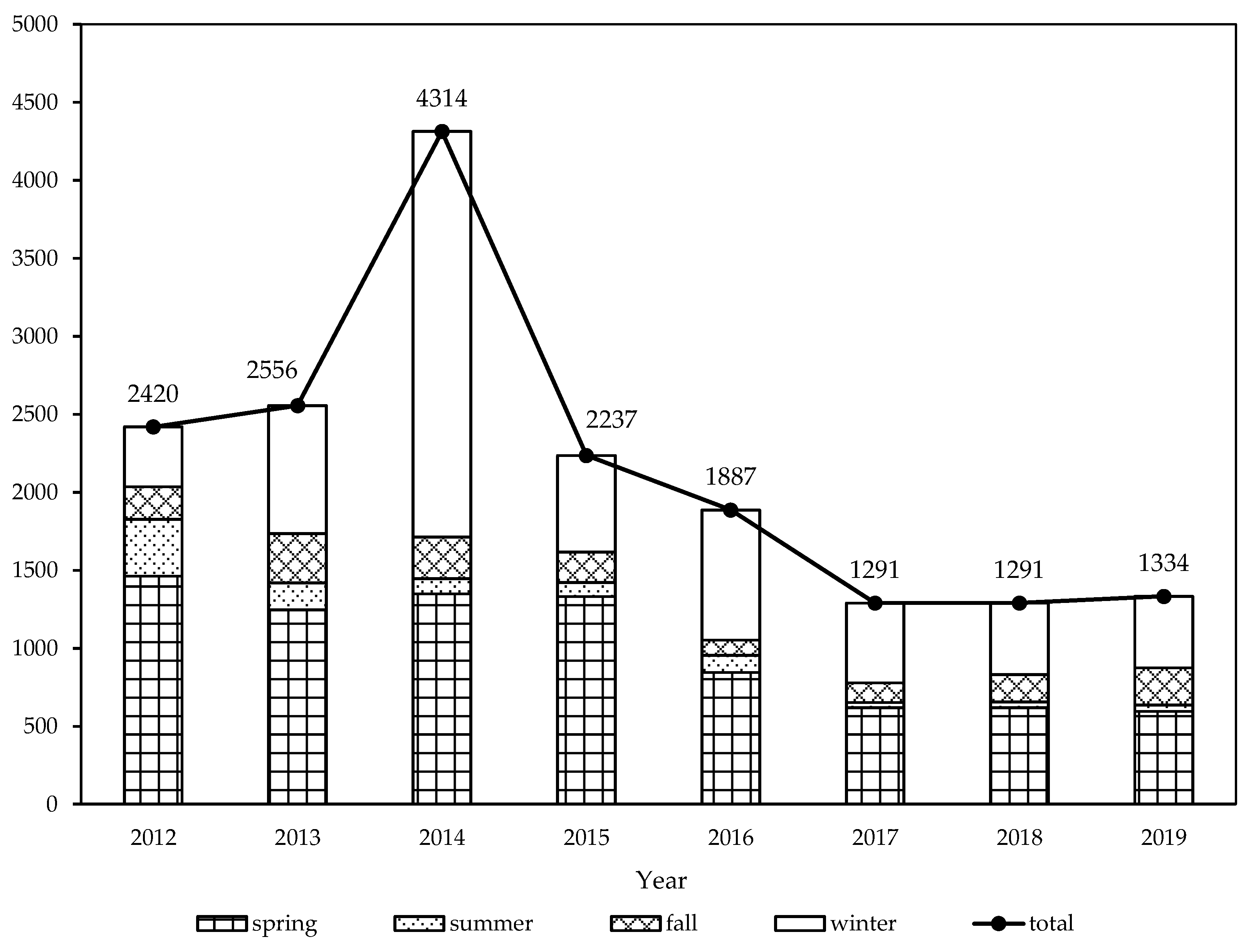
3.2. Forest Fire Statistics in China

As shown in Figure 5, 17,330 fire points under forest cover were recorded in the period 2012–2019. The highest number was 4314 in 2014, whereas the lowest was 1291 in 2017 and 2018. Regarding quantity, the fire points exhibit a fluctuating downward trend overall. The Chinese government has continuously strengthened the prevention and control of FFs; strengthened the supervision, management, and guidance of the central and local governments, reducing the occurrence of fires from their sources; strengthened the system of FF brigades; and upgraded new technologies and equipment to improve the fire-prevention capacity. The annual pattern can be subdivided into two time periods: rising in 2012–2014 (slowly in 2012–2013 [increase in no. of FF points = 136], rapidly in 2013–2014 [increase in no. of FF points = 1758]) and overall decreasing in 2014–2019 (rapidly in 2014–2015 [decrease in no. of FF points = 2077], slowly in 2015–2019 [average annual decrease in no. of FF points = 180.6]). The seasonal difference is more obvious in Figure 5. From 2012 to 2019, the number of fires in spring, summer, autumn, and winter was 8071, 946, 1621, and 6692, respectively. We divided the fire points into four seasons according to meteorological standards, i.e., spring (March, April, May), summer (June, July, August), fall (September, October, November), and winter (December, January, February). Regarding the seasonal distribution of FFs, spring and winter had the most, and there were fewer fire points in the fall and summer; the number of fire points in spring far exceeded that in the fall, showing that the situation in spring is more severe. In spring, most areas of southern China are busy with spring farming production, with more fire affecting farming, which makes it more difficult to manage fire sources. With the rapid rise of temperature in the northeast and Inner Mongolia forest areas, the southwest is dry, increasing fire risk. It is hot and rainy in summer, with high water content in plants and wet ground cover. In autumn, the dryness of the northern forest increases, and the fallen leaves and dead branches lead to the increase in combustibles. In winter, the forest areas in northern and southern China are dry, and the fire risk level is high.

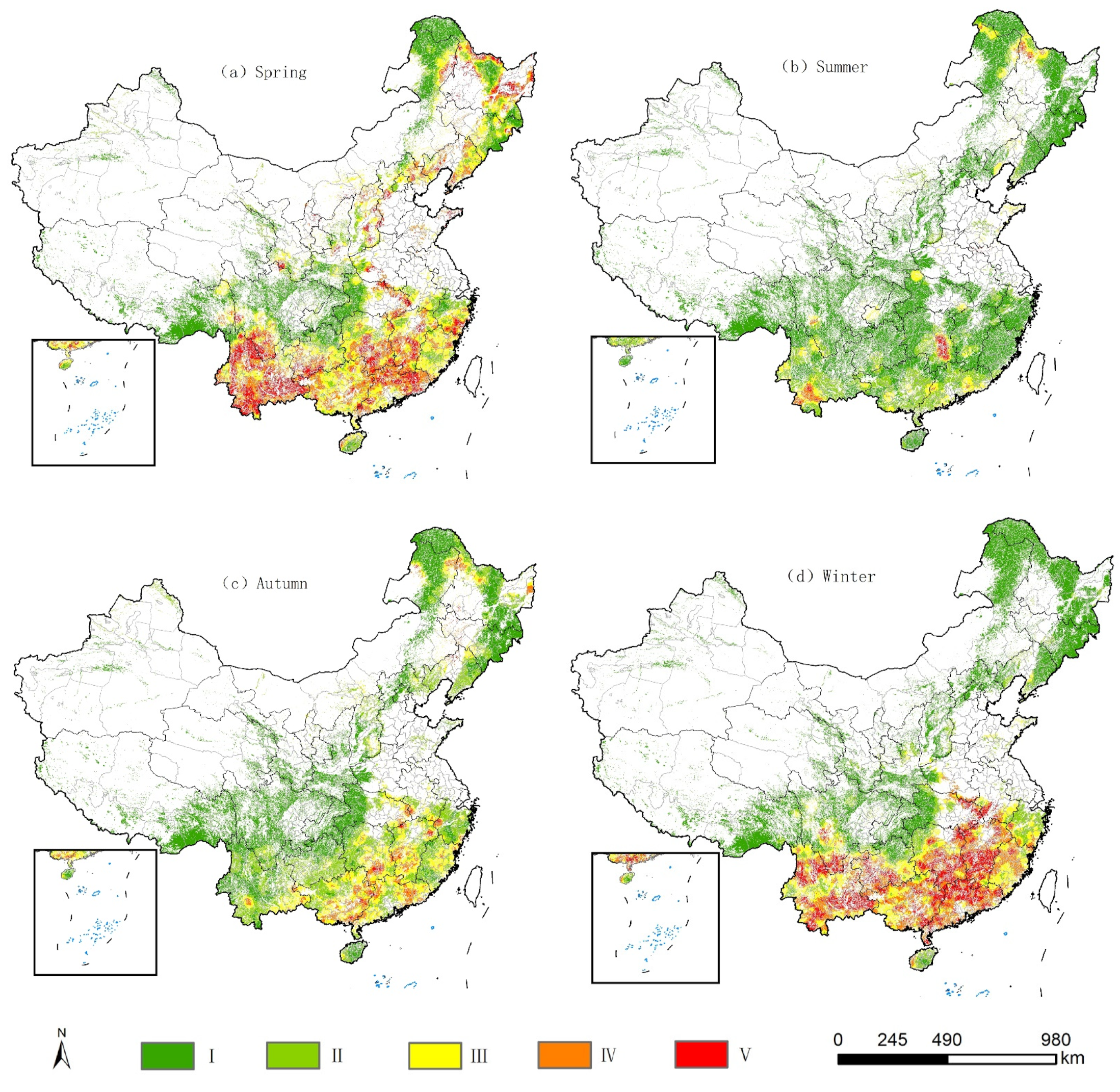
3.3. Seasonal Fire Zoning Map

A better understanding of the spatial distribution of FFs is essential for effective fire management, enabling the optimal allocation of fire resources. We selected the best-performing RF model to map China’s seasonal fire risk. Fire prediction probabilities were subsequently interpolated using the kriging interpolation method in the ArcGIS 10.4 software. This process yields a reasonable relationship between the real and estimated values and the lowest mean square error compared to other commonly used interpolation methods. It can maximize the use of the information during spatial sampling and consider the positional relationship between the sampling points, effectively avoiding the occurrence of systematic errors [65], with focused monitoring in fire-prone areas. The fire-risk areas in the present study were divided into five categories (I–V) for FF risk zoning: I) the probability range of 0.0–0.2 means that FFs essentially do not occur; II) the probability range of 0.2–0.4 means that FFs do not happen easily; III) the probability range of 0.4–0.6 means that FFs may happen; IV) the probability range of 0.6–0.8 indicates that FFs happen easily; V) the probability range of 0.8–1.0 means that FFs happen very easily.

In Figure 6, the seasonal spatial zoning of the FF risk show that the order is spring > winter > summer > fall. In this regard, the spring level-V fire-risk areas are mainly in Yunnan Province (e.g., the cities of Qujing, Lijiang, and Yuxi, and the autonomous prefectures of Dali Bai, Nujiang Lisu, Wenshan Zhuang and Miao, and Honghe Hani and Yi), Guangdong Province (e.g., the cities of Shaoguan, Huizhou, Qingyuan, Jieyang, and Heyuan), Guangxi Province (e.g., the cities of Nanning, Liuzhou, and Baise), Hunan Province (e.g., the regions of Yongzhou, Hengyang, Loudi, and Shaoyang), Hubei Province (e.g., the cities of Suizhou, Huangshi, and Huanggang), the northeast region (e.g., the cities of Heihe, Qitaihe, Dandong, and Jinzhou), Inner Mongolia (e.g., the eastern part of the city of Hulunbuir), and southern Sichuan Province (e.g., part of the Liangshan Yi Autonomous Prefecture). The spring level-IV fire-risk areas are mainly in Chuxiong, Yunnan, Guangxi (Hechi, Yulin, Chongzuo), Qamdo, Tibet, and Fujian (Ningde, Sanming). The summer level-V fire-risk areas are mainly in Yunnan (Pu’er), Hunan (e.g., Xiangtan, Hengyang), and Guangdong (Huizhou, Zhaoqing). The fall level-V fire-risk areas are mainly in Jiangxi Province (the cities of Jiujiang and Jian), Hubei Province (the city of Huanggang), Guangxi (the cities of Baise and Hezhou), Guangdong (the cities of Zhaoqing and Heyuan), and Hunan Province (the cities of Hengyang and Binzhou). The winter level-V fire-risk areas are mainly in Yunnan Province (e.g., the cities of Lijiang and Yuxi, and the Honghe Hani and Yi Autonomous Prefecture), Guizhou Province (the autonomous prefectures of Qianxinan Buyi and Miao and Qiannan Buyi and Miao, and the city of Bijie), Guangxi (Yulin, Nanning, Liuzhou), Guangdong Province (Qingyuan, Shaoguan, Heyuan, Huizhou), Hunan Province (Changde, Yongzhou, Shaoyang, Hengyang City), Jiangxi Province (Ganzhou, Fuzhou, Jiujiang, etc.), and Fujian Province (Nanping). In general, fire prevention in China is essential in spring and winter, and prevention should be strengthened, especially in the above vital cities. Note that parts of northeast China (e.g., the cities of Heihe, Qitaihe, and Dandong) are at high risk of FFs in spring and the fall.

China’s FF risk prediction and zoning show obvious differences in distribution patterns because of the influence of many factors. Because of China’s vast land area, different regions have great differences in topography, climate, and other natural conditions, and the accompanying human activities are also different, which lead to large regional differences in the risk of FFs. Northeast China (e.g., the cities of Heihe, Qitaihe, and Dandong) is rich in forest resources, and there is a typical monsoon climate every spring and fall; the spring climate is dry, and there are strong winds, less precipitation, and low relative humidity in the fall, which increases the probability and duration of fire outbreaks [66].

Parts of the northeast and Inner Mongolia are in high-risk areas that are flat. Because of Siberia, the spring and fall seasons there are windy and inconvenient for transportation, so it is difficult for firefighters to reach a fire in time before it spreads rapidly. Wind causes widespread FF risk [67]. Northwest China (the provinces of Gansu, Ningxia, Qinghai, Shanxi, and Xinjiang) has fewer FFs because of its lack of forest resources and low population density, so the risk is low. Southwest China (e.g., the provinces of Sichuan, Yunnan, and Guizhou, and the city of Chongqing) is a high-risk area for FFs. The terrain there is complex and mainly mountainous, with high mountains, dense forests, and rich vegetation types. It has a subtropical monsoon climate, with dry and windy weather in winter and spring, and dry weather often occurs [68]. In southern China, some high-risk areas in Guangdong and Fujian are rich in forest resources, with developed economies, high population density, accelerated urbanization, and a large influx of labor. Forests and farms are collocated, and agriculture and negligent use of fire in southern China have become the main sources of FFs there [69].

4. Discussion

Large-scale FF modeling is a nonlinear and complex problem that is not easy to evaluate and predict. As shown in

Table 2. Suitability of classifiers in FF modeling according to previous studies.

No	Methods Used	Best Method	Study Area	Ref.
1	Generalized linear models, RF, maximum entropy	Maximum entropy	Huron–Manistee National Forest, MI, USA	[70]
2	RF, extreme gradient boosting	RF	Montesinho Natural Park, Portugal	[71]
3	Logistic regression, NN	NN	Central Portugal	[72]
4	RF, boosting regression trees, SVMs, logistic regression	RF	Lào Cai province, Vietnam	[73]
5	Multiple linear regression and RF	RF	Mediterranean Europe	[74]
6	Cascade correlation network, MLP NN, polynomial NN, RBF, SVM	SVM	Montesinho Natural Park, Portugal	[75]
7	Bayes network, naïve Bayes, decision tree, multivariate logistic regression	Multivariate logistic regression	Pu Mat National Park, Vietnam	[76]
8	Frequency ratio–multilayer perceptron, frequency ratio–classification and regression tree, frequency ratio–support vector machine, frequency ratio–RF	Frequency ratio–RF	Tanger-Tétouan-Al Hoceima region, northern Morocco	[77]
9	Artificial NN, SVM, RF	RF	Amol County, Iran	[78]
10	Artificial NN, SVM	Artificial NN	Guangxi, China	[79]

, different scholars have conducted numerous studies to assess the applicability of various methods [70,71,72,73,74,75,76,77,78,79]. Using four ML methods and 20 variables, we computed and compared the performance of the different models and reported the results of the predictive models. Our results suggest that the RF algorithm performs the best of the four ML methods, followed by GBDT and MLP, with SVM being the worst. The RF algorithm can operate quickly and with high accuracy on large datasets with numerous predictive variables. Among its various advantages, RF has high precision, can handle high-dimensional samples without factor screening, can handle noisy or missing data, has high training and prediction speed, can handle high-dimensional data, and is effective for eliminating model overfitting [71,73,78]. However, unlike decision trees, the RF model is not easily explained. Some work may be needed to tune the data model, such as testing different parameters and random seeds. Moreover, it may not yield a good classification for small or low-dimension data (data with fewer features).

In contrast, SVM has the advantage of capturing complex and nonlinear relationships. However, we found it to be inefficient, time consuming, and cumbersome in handling large samples. This is consistent with previous research [73]. In addition, in the present study, GBDT performed worse than RF and better than SVM. Compared with SVM, GBDT had a higher predictive accuracy with less tuning time. Because of the dependence between weak learners, it is difficult to train the data in parallel, and the higher the data dimension, the greater the computational complexity of the algorithm. MLP can handle parallel training of data with global optimization. In the present study, MLP outperformed SVM but performed worse than RF and GBDT. GBDT could not reach the accuracy of RF without adjustment of its parameters. RF repeatedly selects random subsamples from the original training samples to construct multiple decision trees by using bootstrap resampling, whereas the minimization loss function of the GBDT model is calculated iteratively to determine the parameters of the next weak classifier to obtain the optimal solution. Without parameter adjustment, the GBDT model applies all the samples to each weak classifier, which increases the variance and produces overfitting [54]. As black-box models for machine learning, both the RF and GBDT models can accommodate the large number of features used for training. Our research on predicting fire risk based on ML will generate information that will help to (i) support fire management, (ii) allocate resources rationally, and (iii) reduce the time and cost of prevention efforts.

China’s FF points generally show a fluctuating and downward trend. The spatial and temporal distributions of FF risks in China are concentrated, with spring and winter being the high-risk seasons for FF risk in China. The high-risk areas of FF are mainly concentrated in northeast, southwest, and southern China, which is consistent with previous studies [11]. For such areas with high risk of FFs, it is suggested to increase investment, improve the FF prevention and control capacity in key areas, and ensure the safety of forest resources. (i) The high-risk areas for FFs in Inner Mongolia and northeastern China (e.g., the cities of Heihe, Qitaihe, and Dandong) are relatively flat. Because of the dense distribution of forest resources, high coverage, flat terrain, drought and wind in spring and fall, and less rainfall, these areas are prone to heavy and extra-large FFs [67]. A focus on the equipment and construction of mechanized FF brigades is suggested to improve the density of road networks, strengthen the prediction of lightning fires, and improve the ability to deal with heavy and extra-large FFs. (ii) For the high-risk area for FFs in southwestern China (e.g., the cities of Qujing, Lijiang, and Yuxi), because of the complex terrain and dry and windy climate in winter and spring, it is difficult to put out a fire if one happens [68]. This area must focus on the equipment and construction of mechanized FF brigades, which should be equipped with large machinery suitable for the topographic conditions, such as digging belt openers and bulldozers, and equipped with large and medium-sized helicopters suitable for high altitudes [80]. (iii) For areas with a high risk of FFs, such as southern China (e.g., Qingyuan, Shaoguan, Heyuan, Huizhou) [69], forest farmers are considerably intertwined, and human activities are frequent. The watchtowers and FF video monitoring system must be improved to advance the FF observation and monitoring ability, fire-prevention publicity and education must be enhanced, and the ability to deal with FFs locally and quickly must be addressed [80].

FF prediction is an integral part of managing emergency responses, and mapping areas that are vulnerable to fire will help determine the focus of hazard management and mitigate FF hazards. However, the accuracy of each fire-risk forecast differs depending on the quality of the data, the method used, and additional input parameters. In the present study, we used four ML methods, and the results show that the SVM model is not suitable for fire-risk research in our study area. However, this may differ for other research areas and fields. Different models have their own advantages and disadvantages, depending on the availability and number of training data [81,82]. However, there is no evidence that a particular model is optimal for specific hazards, as this also depends on the study area and the available data from that specific region. How the number of training data points affects the performance of each ML method remains unclear and is a possible limitation of the present study, where no combustion-related data studies were added to FF risk prediction. When there is no more-accurate forest-vegetation data, NDVI/FVC data are widely used. In future work, we hope to obtain and use more-accurate vegetation species and combustion and soil-moisture data for modeling prediction studies [83,84].

5. Conclusions

It is difficult to obtain data sources with long time series, high precision, and unified temporal and spatial resolution in China. Therefore, this will also have a certain impact on the research accuracy. In spite of this limitation, predicting fires is an integral part of dealing with emergencies, and timely mapping and management of areas and prioritizing risks will help mitigate the impact of a fire. ML and geographic information systems are essential tools for large-scale fire-risk analysis and mapping. The present study provided a large-scale FF risk prediction framework with low cost, high precision, and high operability. We comprehensively compared four ML methods to predict Chinese FF risks based on confidence fire points from 2012 to 2019. Based on this, we selected the best-performing RF method to map zoning of FFs in China.

The results will help management departments to understand the locations, characteristics, frequency, severity, and seasonality of FFs in China. Our research results provide an effective map for zoning China to prioritize resource allocation of FF risk management plans. In addition, different fire prevention and management strategies must provide more appropriate, locally specific management plans and strategies. Future plans include investigating and developing different method/model combinations capable of predicting FFs by combining the strong penetrating ability of microwave remote-sensing data and sensitivity to surface moisture [85]. We also plan to build a daily high-spatial-resolution prediction model for the high-incidence areas of FFs, couple this to a hybrid model of an artificial-intelligence algorithm and an optimization algorithm, and introduce it into the FF prediction model to improve the prediction accuracy and robustness.

References

1. Morales-Hidalgo, D.; Oswalt, S.N.; Somanathan, E. Status and trends in global primary forest, protected areas, and areas designated for conservation of biodiversity from the Global Forest Resources Assessment 2015. For. Ecol. Manag. 2015, 352, 68–77. [Google Scholar] [CrossRef] [Green Version]
2. Qiu, Z.; Feng, Z.; Song, Y.; Li, M.; Zhang, P. Carbon sequestration potential of forest vegetation in China from 2003 to 2050: Predicting Forest vegetation growth based on climate and the environment. J. Clean. Prod. 2019, 252, 119715. [Google Scholar] [CrossRef]
3. Motazeh, A.G.; Ashtiani, E.F.; Baniasadi, R.; Choobar, F.M. Rating and mapping fire hazard in the hardwood Hyrcanian forests using GIS and expert choice software. For. Ideas. 2013, 19, 141–150. [Google Scholar]
4. Ke, Z.; Gebdang, B.; Xin, L.B.; Zhijia, B.; Zhongbo, Y.; Jun, X.; Zengchuan, D. A comprehensive assessment framework for quantifying climatic and anthropogenic contributions to streamflow changes: A case study in a typical semi-arid North China basin. Environ. Model. Softw. 2020, 128, 104704. [Google Scholar]
5. Feng, W.; Lu, H.; Yao, T.; Yu, Q. Drought characteristics and its elevation dependence in the Qinghai–Tibet plateau during the last half-century. Sci. Rep. 2020, 10, 14323. [Google Scholar] [CrossRef]
6. Zheng, Z. Study on the risk, spread and assessment of forest fire based on the model and remote sensing. Acta Geod. Cartogr. Sin. 2019, 48, 133. [Google Scholar]
7. Sachdeva, S.; Bhatia, T.; Verma, A.K. GIS-based evolutionary optimized gradient boosted decision trees for forest fire susceptibility mapping. Nat. Hazards 2018, 92, 1399–1418. [Google Scholar] [CrossRef]
8. Boer, M.M.; Dios, V.; Bradstock, R.A. Unprecedented burn area of Australian mega forest fires. Nat. Clim. Chang. 2020, 10, 171–172. [Google Scholar] [CrossRef]
9. Venkatesh, K.; Preethi, K.; Ramesh, H. Evaluating the effects of forest fire on water balance using fire susceptibility maps. Ecol. Indic. 2019, 110, 105856. [Google Scholar] [CrossRef]
10. Ghorbanzadeh, O.; Blaschke, T.; Gholamnia, K.; Aryal, J. Forest fire susceptibility and risk mapping using social/infrastructural vulnerability and environmental variables. Fire 2019, 2, 50. [Google Scholar] [CrossRef] [Green Version]
11. Ma, W.; Feng, Z.; Cheng, Z.; Chen, S.; Wang, F. Identifying forest fire driving factors and related impacts in China using random forest algorithm. Forests 2020, 5, 507. [Google Scholar] [CrossRef]
12. Kuuluvainen, T.; Grenfell, R. Natural disturbance emulation in boreal forest ecosystem management—theories, strategies, and a comparison with conventional even-aged management. Can. J. For. Res. 2012, 42, 1185–1203. [Google Scholar] [CrossRef]
13. Moreno, M.V.; Chuvieco, E. Characterising fire regimes in Spain from fire statistics. Int. J. Wildland Fire 2013, 22, 296–305. [Google Scholar] [CrossRef]
14. González, J.R.; Kolehmainen, O.; Pukkala, T. Using expert knowledge to model forest stand vulnerability to fire. Comput. Electron. Agric. 2007, 55, 107–114. [Google Scholar] [CrossRef]
15. Stock, M.; Williams, J.; Cleaves, D.A. Estimating the risk of escape of prescribed fires: An expert system approach. AI Appl. Nat. Resour. Agric. Environ. Sci. 1996, 10, 63. [Google Scholar]
16. Jaafari, A.; Mafi-Gholami, D.; Thai Pham, B.; Tien Bui, D. Wildfire Probability Mapping: Bivariate vs. Multivariate Statistics. Remote Sens. 2019, 11, 618. [Google Scholar] [CrossRef] [Green Version]
17. Su, Z.; Zeng, A.; Cai, Q.; Hu, H. Study on prediction model and driving factors of forest fire in Da Hinggan Mountains using Gompit regression method. J. For. Eng. 2019, 4, 135–142. [Google Scholar]
18. Rodrigues, M.; Riva, J.D.L.; Fotheringham, S. Modeling the spatial variation of the explanatory factors of human-caused wildfires in Spain using geographically weighted logistic regression. Appl. Geogr. 2014, 48, 52–63. [Google Scholar] [CrossRef]
19. Pourghasemi, H.R. GIS-based forest fire susceptibility mapping in Iran: A comparison between evidential belief function and binary logistic regression models. Scand. J. For. Res. 2015, 31, 80–98. [Google Scholar] [CrossRef]
20. Qin, K.; Guo, F.; Di, X.; Sun, L.; Pan, J. Selection of advantage prediction model for forest fire occurrence in Tahe, Daxing’an Mountain. Chin. J. Appl. Ecol. 2014, 25, 731–737. [Google Scholar]
21. Boubeta, M.; Lombardia, M.J.; Marey-Perez, M.F.; Morales, D. Prediction of forest fires occurrences with area-level Poisson mixed models. J. Environ. Manag. 2015, 154, 151–158. [Google Scholar] [CrossRef] [PubMed]
22. Jaafari, A.; Gholami, D.M. Wildfire hazard mapping using an ensemble method of frequency ratio with Shannon’s entropy. Iran. J. For. Poplar Res. 2017, 25, 232–242. [Google Scholar]
23. Gholamnia, K.; Gudiyangada Nachappa, T.; Ghorbanzadeh, O.; Blaschke, T. Comparisons of diverse machine learning approaches for wildfire susceptibility mapping. Symmetry 2020, 12, 604. [Google Scholar] [CrossRef] [Green Version]
24. Sayad, Y.O.; Mousannif, H.; Al Moatassime, H. Predictive modeling of wildfires: A new dataset and machine learning approach. Fire Saf. J. 2019, 104, 130–146. [Google Scholar] [CrossRef]
25. Song, Y.; Liu, B.; Miao, W.; Chang, D.; Zhang, Y. Spatiotemporal variation in nonagricultural open fire emissions in China from 2000 to 2007. Global Biogeochem. Cycles 2009, 23. [Google Scholar] [CrossRef]
26. Adab, H.; Kanniah, K.D.; Solaimani, K. Modeling forest fire risk in the northeast of Iran using remote sensing and GIS techniques. Nat. Hazards 2013, 65, 1723–1743. [Google Scholar] [CrossRef]
27. Yu, C.; Zhu, Z.; Bu, R.; Chen, H.; Wang, Z. Predicting fire occurrence patterns with logistic regression in Heilongjiang Province, China. Landsc. Ecol. 2013, 28, 1989–2004. [Google Scholar]
28. Ying, L.; Han, J.; Du, Y.; Shen, Z. Forest fire characteristics in China: Spatial patterns and determinants with thresholds. For. Ecol. Manag. 2018, 424, 345–354. [Google Scholar] [CrossRef]
29. Morgan, P.; Hardy, C.C.; Swetnam, T.W.; Rollins, M.G.; Long, D.G. Mapping fire regimes across time and space: Understanding coarse and fine-scale fire patterns. Int. J. Wildland Fire 2001, 10, 329–342. [Google Scholar] [CrossRef] [Green Version]
30. Sun, J.; Zhong, C.; He, H.; Hugeman, G.; Li, H. Continuous remote sensing monitoring and changes of land desertification in China from 2000 to 2015. J. Northeast. For. Univ. 2021, 49, 87–92. [Google Scholar]
31. Unnikrishnan, A.; Reddy, C.S. Characterizing distribution of forest fires in Myanmar using earth observations and spatial statistics tool. J. Indian Soc. Remote Sens. 2020, 48, 227–234. [Google Scholar] [CrossRef]
32. Ning, J.; Liu, J.; Kuang, W.; Xu, X.; Zhang, S.; Yan, C.; Li, R.; Wu, S.; Hu, Y.; Du, G.; et al. Spatiotemporal patterns and characteristics of land-use change in China during 2010–2015. J. Geogr. Sci. 2018, 28, 547–562. [Google Scholar] [CrossRef] [Green Version]
33. Guo, F.; Su, Z.; Wang, G.; Sun, L.; Tigabu, M.; Yang, X.; Hu, H. Understanding fire drivers and relative impacts in different Chinese forest ecosystems. Sci. Total Environ. 2017, 605–606, 411–425. [Google Scholar] [CrossRef] [PubMed]
34. Holden, Z.A.; Jolly, W.M. Modeling topographic influences on fuel moisture and fire danger in complex terrain to improve wildland fire management decision support. For. Ecol. Manag. 2011, 262, 2133–2141. [Google Scholar] [CrossRef]
35. Wu, Z.; He, H.S.; Yang, J.; Liu, Z.; Liang, Y. Relative effects of climatic and local factors on fire occurrence in boreal forest landscapes of northeastern China. Sci. Total Environ. 2014, 493, 472–480. [Google Scholar] [CrossRef]
36. Sun, Y.L.; Shan, M.; Pei, X.R.; Zhang, X.K.; Yang, Y.L. Assessment of the impacts of climate change and human activities on vegetation cover change in the Haihe River basin, China. Phys. Chem. Earth 2020, 115, 102834. [Google Scholar] [CrossRef]
37. Gutman, G.; Ignatov, A. The derivation of the green vegetation fraction from NOAA/AVHRR data for use in numerical weather prediction models. Int. J. Remote Sens. 1998, 19, 1533–1543. [Google Scholar] [CrossRef]
38. Guo, F.; Wang, G.; Su, Z.; Liang, H.; Wang, W.; Lin, F. What drives forest fire in Fujian, China? Evidence from logistic regression and random forests. Int. J. Wildland Fire 2016, 25, 505. [Google Scholar] [CrossRef]
39. Gigović, L.; Pourghasemi, H.R.; Drobnjak, S.; Bai, S. Testing a new ensemble model based on SVM and random forest in forest fire susceptibility assessment and its mapping in Serbia’s Tara National Park. Forests 2019, 10, 408. [Google Scholar] [CrossRef] [Green Version]
40. Ma, Z.C.; Yu, H.B.; Cao, C.M.; Zhang, Q.F.; Hou, L.L.; Liu, Y.X. Spatio temporal Characteristics of Fractional Vegetation Coverage and Its Influencing Factors in China. Resour. Environ. Yangtze Val. 2020, 29, 12. [Google Scholar]
41. Ma, W.; Feng, Z.; Cheng, Z.; Chen, S.; Wang, F. Study on driving factors and distribution pattern of forest fires in Shanxi province. J. Cent. South Univ. For. Technol. 2020, 40, 57–69. [Google Scholar]
42. Breiman, L. Random forests. Mach. Learn. 2001, 45, 5–32. [Google Scholar] [CrossRef] [Green Version]
43. Diao, C.; Wang, L. Incorporating plant phenological trajectory in exotic saltcedar detection with monthly time series of Landsat imagery. Remote Sens. Environ. 2016, 182, 60–71. [Google Scholar] [CrossRef]
44. Shi, H. Best-First Decision Tree Learning. Master’s Thesis, University of Waikato, Hamilton, New Zealand, 2007. Available online: https://hdl.handle.net/10289/2317 (accessed on 24 February 2007).
45. Vapnik, V. The support vector method of function estimation. In Nonlinear Modeling: Advanced Black-Box Techniques; Suykens, J.A.K., Vandewalle, J., Eds.; Springer: Boston, MA, USA, 1998; pp. 55–85. [Google Scholar]
46. Negri, R.G.; Dutra, L.V.; Sant’Anna, S.J.S. An innovative support vector machine based method for contextual image classification. ISPRS J. Photogramm. Remote Sens. 2014, 87, 241–248. [Google Scholar] [CrossRef]
47. Belousov, A.I.; Verzakov, S.A.; von Frese, J. Applicational aspects of support vector machines. J. Chemom. 2010, 16, 482–489. [Google Scholar] [CrossRef]
48. Vapnik, V.N. An overview of statistical learning theory. IEEE Trans. Neural Netw. 1999, 10, 988–999. [Google Scholar] [CrossRef] [Green Version]
49. Maser, B.; Söllinger, D.; Uhl, A. PRNU-based finger vein sensor identification in the presence of presentation attack data. In Proceedings of the Joint ARW/OAGM Workshop 2019 (ARW/OAGM’19), Steyr, Austria, 9–10 May 2019. [Google Scholar]
50. Araujo, L.N.; Belotti, J.T.; Alves, T.A.; Tadano, Y.D.S.; Siqueira, H. Ensemble method based on artificial neural networks to estimate air pollution health risks. Environ. Model. Softw. 2020, 123, 104567. [Google Scholar] [CrossRef]
51. Feng, R.; Gao, H.; Luo, K.; Fan, J.R. Analysis and accurate prediction of ambient PM2.5 in China using multi-layer perceptron. Atmos. Environ. 2020, 232, 117534. [Google Scholar] [CrossRef]
52. Zhang, T.; He, W.; Zheng, H.; Cui, Y.; Song, H.; Fu, S. Satellite-based ground PM2.5 estimation using a gradient boosting decision tree. Chemosphere 2021, 268, 128801. [Google Scholar] [CrossRef]
53. Friedman, J. Greedy function approximation: A gradient boosting machine. Ann. Stat. 2001, 29, 1189–1232. [Google Scholar] [CrossRef]
54. Rong, G.; Alu, S.; Li, K.; Su, Y.; Li, T. Rainfall induced landslide susceptibility mapping based on Bayesian optimized random forest and gradient boosting decision tree models—A case study of Shuicheng County, China. Water 2020, 12, 3066. [Google Scholar] [CrossRef]
55. Yang, S.; Wu, J.; Du, Y.; He, Y.; Chen, X. Ensemble learning for short-term traffic prediction based on gradient boosting machine. J. Sens. 2017, 2017, 7074143. [Google Scholar] [CrossRef]
56. Takran, T.; Chartrungruang, B.; Tantranont, N.; Somhom, S. Constructing a Thai homestay standard assessment model by implementing a decision tree technique. Int. J. Comput. Internet Manag. 2017, 25, 106–112. [Google Scholar]
57. Swets, J. Measuring the accuracy of diagnostic systems. Science 1988, 240, 1285–1293. [Google Scholar] [CrossRef] [Green Version]
58. Gigliarano, C.; Figini, S.; Muliere, P. Making classifier performance comparisons when ROC curves intersect. Comput. Stat. Data Anal. 2014, 77, 300–312. [Google Scholar] [CrossRef]
59. Bui, D.T.; Shirzadi, A.; Shahabi, H.; Geertsema, M.; Lee, S. New ensemble models for shallow landslide susceptibility modeling in a semi-arid watershed. Forests 2019, 10, 743. [Google Scholar]
60. Genuer, R.; Poggi, J.M.; Tuleau-Malot, C. Variable selection using random forests. Pattern Recognit. Lett. 2010, 31, 2225–2236. [Google Scholar] [CrossRef] [Green Version]
61. Chuvieco, E.; Cocero, D.; Riaño, D.; Martin, P.; Martínez-Vega, J.; de la Riva, J.; Pérez, F. Combining NDVI and surface temperature for the estimation of live fuel moisture content in forest fire danger rating. Remote Sens. Environ. 2004, 92, 322–331. [Google Scholar] [CrossRef]
62. Vasilakos, C.; Kalabokidis, K.; Hatzopoulos, J.; Matsinos, I. Identifying wildland fire ignition factors through sensitivity analysis of a neural network. Nat. Hazards 2009, 50, 125–143. [Google Scholar] [CrossRef]
63. Holsten, A.; Dominic, A.R.; Costa, L.; Kropp, J.P. Evaluation of the performance of meteorological forest fire indices for German federal states. For. Ecol. Manag. 2013, 287, 123–131. [Google Scholar] [CrossRef]
64. Vilar, L.; Woolford, D.G.; Martell, D.L.; MP Martín. A model for predicting human-caused wildfire occurrence in the region of Madrid, Spain. Int. J. Wildland Fire 2010, 19, 325–337. [Google Scholar] [CrossRef]
65. Eugenio, F.C.; Santos, A.D.; Fiedler, N.C.; Ribeiro, G.A.; Silva, A.; Dos Santos, Á.B.; Paneto, G.G.; Schettino, V.R. Applying GIS to develop a model for forest fire risk: A case study in Espírito Santo, Brazil. J. Environ. Manag. 2016, 173, 65–71. [Google Scholar] [CrossRef] [PubMed]
66. Li, X.; He, H.S.; Wu, Z.; Liang, Y.; Schneiderman, J.E. Comparing effects of climate warming, fire, and timber harvesting on a boreal forest landscape in northeastern China. PLoS ONE 2013, 8, e59747. [Google Scholar] [CrossRef] [PubMed] [Green Version]
67. Zhong, M.; Fan, W.; Liu, T.; Li, P. Statistical analysis on current status of China forest fire safety. Fire Saf. J. 2003, 38, 257–269. [Google Scholar] [CrossRef]
68. Yi, K.; Bao, Y.; Zhang, J. Spatial distribution and temporal variability of open fire in China. Int. J. Wildland Fire. 2016, 26, 122–135. [Google Scholar] [CrossRef] [Green Version]
69. Fang, K.; Yao, Q.; Guo, Z.; Zheng, B.; Trouet, V. ENSO modulates wildfire activity in China. Nat. Commun. 2021, 12, 1764. [Google Scholar] [CrossRef]
70. Massada, A.B.; Syphard, A.D.; Stewart, S.I.; Radeloff, V.C. Wildfire ignition-distribution modelling: A comparative study in the Huron–Manistee National Forest, Michigan, USA. Int. J. Wildland Fire 2013, 22, 174–183. [Google Scholar] [CrossRef]
71. Xie, Y.; Peng, M. Forest fire forecasting using ensemble learning approaches. Neural Comput. Appl. 2019, 31, 4541–4550. [Google Scholar] [CrossRef]
72. Vasconcelos, M.J.P.D.; Silva, S.; Tome, M.; Alvim, M.; Pereira, J.M.C. Spatial prediction of fire ignition probabilities: Comparing logistic regression and neural networks. Photogramm. Eng. Remote Sens. 2001, 67, 73–81. [Google Scholar]
73. Rodrigues, M.; de la Riva, J. An insight into machine-learning algorithms to model human-caused wildfire occurrence. Environ. Model. Softw. 2014, 57, 192–201. [Google Scholar] [CrossRef]
74. Oliveira, S.; Oehler, F.; San-Miguel-Ayanz, J.; Camia, A.; Pereira, J.M. Modeling spatial patterns of fire occurrence in Mediterranean Europe using multiple regression and random forest. For. Ecol. Manag. 2012, 275, 117–129. [Google Scholar] [CrossRef]
75. Al Janabi, S.; Al Shourbaji, I.; Salman, M.A. Assessing the suitability of soft computing approaches for forest fires prediction. Appl. Comput. Inform. 2018, 14, 214–224. [Google Scholar]
76. Pham, B.T.; Jaafari, A.; Avand, M.; Al-Ansari, N.; Dinh Du, T.; Yen, H.P.H.; Phong, T.V.; Nguyen, D.H.; Le, H.V.; Mafi-Gholami, D.; et al. Performance evaluation of machine learning methods for forest fire modeling and prediction. Symmetry 2020, 12, 1022. [Google Scholar] [CrossRef]
77. Mohajane, M.; Costache, R.D.; Karimi, F.; Pham, Q.B.; Essahlaoui, A.; Nguyen, H.; Laneve, G.; Oudija, F. Application of remote sensing and machine learning algorithms for forest fire mapping in a Mediterranean area. Ecol. Indic. 2021, 129, 1–17. [Google Scholar] [CrossRef]
78. Ghorbanzadeh, O.; Valizadeh Kamran, K.; Blaschke, T.; Aryal, J.; Naboureh, A.; Einali, J.; Bian, J. Spatial prediction of wildfire susceptibility using field survey GPS data and machine learning approaches. Fire 2019, 2, 43. [Google Scholar] [CrossRef] [Green Version]
79. Li, Y.; Feng, Z.; Chen, S.; Zhao, Z.; Wang, F. Application of the artificial neural network and support vector machines in forest fire prediction in the Guangxi Autonomous Region, China. Discrete Dyn. Nat. Soc. 2020, 2020, 5612650. [Google Scholar] [CrossRef] [Green Version]
80. Gao, J. Middle and long term plan discussion of key problems to forest fire prevention in China. For. Inventory Plan. 2015, 40, 4. [Google Scholar]
81. Jaafari, A.; Razavi Termeh, S.V.; Bui, D.T. Genetic and firefly metaheuristic algorithms for an optimized neuro-fuzzy prediction modeling of wildfire probability. J. Environ. Manag. 2019, 243, 358–369. [Google Scholar] [CrossRef]
82. Tien Bui, D.; Hoang, N.-D.; Samui, P. Spatial pattern analysis and prediction of forest fire using new machine learning approach of multivariate adaptive regression splines and differential flower pollination optimization: A case study at Lao Cai province (Viet Nam). J. Environ. Manag. 2019, 237, 476–487. [Google Scholar] [CrossRef]
83. Field, R.D. Evaluation of Global Fire Weather Database reanalysis and short-term forecast products. Nat. Hazard Earth Syst. 2020, 20, 1123–1147. [Google Scholar] [CrossRef]
84. Pettinari, M.L.; Chuvieco, E. Generation of a global fuel data set using the Fuel Characteristic Classification System. Biogeosciences 2016, 13, 2061–2076. [Google Scholar] [CrossRef] [Green Version]
85. Fan, L.; Wigneron, J.P.; Xiao, Q.; Al-Yaari, A.; Wen, J.; Martin-StPaul, N.; Dupuy, J.L.; Pimont, F.; Al Bitar, A.; Fernandez-Moran, R.; et al. Evaluation of microwave remote sensing for monitoring live fuel moisture content in the Mediterranean region. Remote Sens. Environ. 2018, 205, 210–223. [Google Scholar] [CrossRef]
Figure 1. Study area (map) and locations of forest fire (FF) ignitions from NASA’s Fire Information for Resource Management System (https://earthdata.nasa.gov/firms, accessed on 1 January 2022).
Forests 13 00856 g001
Figure 2. Flowchart of methodology used in present study.
Forests 13 00856 g002
Figure 3. Comparison of the precision levels of the four machine learning (ML) models.
Forests 13 00856 g003
Figure 4. Influences of factors on the fire risk model.
Forests 13 00856 g004
Figure 5. Annual and quarterly changes in high-confidence FFs.
Forests 13 00856 g005
Figure 6. Seasonal Chinese FF zoning maps (spring, summer, fall, and winter).
Forests 13 00856 g006