Abstract
Accurate estimations of leaf biomass are required to quantify the amount of material and energy exchanged between vegetation and the atmosphere, to enhance the primary productivity of forest stands, and to assess the contributions of vegetation towards the mitigation of global climate change. The leaf biomass of Moso bamboo (Phyllostachys edulis (Carrière) J. Houz) changes dramatically during the year owing to changes in the leaves and the growth of new shoots. Furthermore, the relationship between the leaf biomass of Moso bamboo under cutting the top of the culm and the diameter at breast height (D) and culm height is decoupling, which increases the difficulty of estimating leaf biomass. Consequently, an effective method to accurately estimate the leaf biomass of Moso bamboo under cutting the top of the culm is required. In this study, leaf biomass and other factors (age, D, culm height, crown length, and crown width) were measured for 54 bamboo samples collected from December 2019 to December 2020. Models for predicting the leaf biomass of the Moso bamboo were established using multiple linear regression with two strategies, and their accuracies were evaluated using leave-one-out cross-validation. The results showed that crown length, crown width, and age were highly correlated with leaf biomass, and these were important factors when making estimations. Variation in monthly averaged leaf biomass is significant, with a decreasing trend from January to May and an increasing trend from June to December in off-years. The leaf biomass model that utilized data from the three leaf change periods had a better fit and accuracy, with R2 values of 0.583–0.848 and prediction errors between 8.59% and 24.19%. The model that utilized data for all months had a worse fit and accuracy, with an R2 value of 0.228 and prediction error of 46.79%. The results of this study provide reference data and technical support to help clarify the dynamic changes in Moso bamboo leaf biomass, and therefore, aid in the development of accurate simulations.
1. Introduction
Plant leaves synthesize the organic matter required for growth via photosynthesis and help to drive water and nutrient uptake by the root system [1]. They also play key roles in forests owing to their carbon uptake, oxygen emissions, and contributions to cooling and wind protection [2,3]. Furthermore, because they are highly dynamic carbon reservoirs, leaves are one of the key driving parameters in ecophysiological process models, such as those for nutrient balance [4], as they can reflect the ability of a tree or stand to intercept radiation, absorb carbon dioxide, store carbohydrates, intercept rainfall, evaporate water, and to some extent, accumulate and store nutrients [5]. Therefore, leaf biomass is an important component of the microenvironment, tree growth, and stand dynamics [6]. It can also determine a plant’s potential to absorb and use light energy, the amount of material and energy exchanged between plants and the atmosphere, and is utilized as a key parameter in the study of plant physiological and ecological processes, materials, and energy cycles [7,8,9]. Therefore, accurate assessments of plant leaf biomass are important when quantifying the exchange of carbon and water between plants and the atmosphere, enhancing productivity, and assessing the contributions of vegetation to the mitigation of global climate change [10,11].
Direct harvesting and indirect estimation methods are currently used to determine leaf biomass [12]. Direct harvesting involves felling a tree, separating the branches and the leaves, and then drying and weighing the leaves to obtain the leaf biomass [13]. This is the traditional and most accurate method to obtain leaf biomass, but it is time-consuming and disruptive to the environment, and the accuracy of the results are subject to considerable uncertainty when extended to larger areas [14,15]. Indirect estimation methods are subdivided into remote sensing and biomass modeling methods. Remote sensing estimations are based on the reflectance spectral characteristics of plants, and vegetation index characteristics are used to estimate biomass. This method provides large- and multiscale data for rapid, quantitative assessments of the aboveground biomass of forests at the regional scale and their changes. However, it can also have insufficient estimation accuracy, and there can be uncertainty of the data sources and biomass models [16,17,18].
The biomass modeling approach requires the collection of numerous samples and the processing of large amounts of data in preliminary research to develop mathematical models of leaf biomass and tree measurement factors [19,20], which can then be applied to other similar areas when making estimations [21]. Currently, this is a popular method, as it has a high likelihood of producing accurate results and is less time-consuming and less costly than direct harvesting [12]. Many scholars have estimated leaf biomass using a biomass modeling method, for example, Kittredge [22] used a single factor, diameter at breast height, to predict the leaf biomass of yellow pine species, and the standard error of prediction was only 11.2%. Biomass modeling also commonly uses a combination of variables to measure trees. For example, Loomis et al. [23] used the diameter at breast height and crown ratio as combination variables to model the canopy biomass of species, such as the short leaf pine, and found a correlation coefficient of 0.99 and a standard deviation of 0.081. Socha et al. [7] used tree measurement factors including height, diameter at breast height, incremental section area, age, and crown length to develop empirical equations for the leaf biomass of Pinus sylvestris, resulting in an accurate estimate of plant leaf biomass with model interpretations ranging from 65% to 85%. To simulate changes in leaf biomass dynamics, some scholars have constructed models based on changes in forest tree growth. Cleary et al. [24] found that sagebrush leaf biomass varied with the month of the growing season and that leaf biomass was significantly correlated with the month (p < 0.01). Doughert et al. [5] investigated torch pine, and a logistic equation was used to predict the cumulative growth of leaf biomass by month, and the correlation coefficient reached 0.99, with a percentage deviation of 11.6%. Ross et al. [25] proposed a statistical interpolation method to calculate the leaf area index, downward cumulative leaf area index, and canopy leaf area density for any given day during the plant growing season using plant stem height and time as independent variables. Thus, leaf growth state changes with time; however, to date, only a few studies have focused on a dynamic model for leaf biomass changes with time, and consequently, the construction of a dynamic model reflecting these changes would have both theoretical and practical significance.
Moso bamboo is a major bamboo species that is widely distributed in the tropical and subtropical regions of East and Southeast Asia. The Moso bamboo forests in China account for 84.02% of its global distribution [26]. In recent years, Moso bamboo has received increasing attention because of its fast growth rate, high renewal capacity, and high carbon sequestration potential [27,28,29,30,31,32]. The growth process of Moso bamboo differs from that of other types of vegetation, as after the bamboo shoots undergo their tall growth period, the height, diameter at breast height, and volume are not expected to change significantly [31,33]. Furthermore, Moso bamboo forests experience the phenomenon of on-years and off-years; in on-years, Moso bamboo starts sprouting new bamboo shoots in spring, and they start spreading their leaves in mid to late May when the leaf biomass increases [26,34], and the leaf biomass of the stand canopy increases by approximately 30% in just one month. The leaf changes in off-years start in March, and as the old leaves drop, new leaves start to grow in April–May and fully expand in June, but the sprouting of new leaves time varies with age, as this occurs latest at 1–2 years, earliest at 3–4 years, and somewhere in between these two at 5–6 years. During the leaf change period, Moso bamboo leaf biomass has been found to vary significantly with time, showing a decreasing trend followed by a rapid increase [34,35,36]. Since Moso bamboo leaves are dense and do not shed their leaves in winter, they are prone to bending, breaking, and falling down when exposed to continuing snow and freezing weather [37]. This results in serious damage to the productivity of Moso bamboo stands. Obtruncation, which means cutting off a part of the culm top, is a widely used management pruning measure to increase the resistance of Moso bamboo to snow damage in China [38,39]. Usually, the length of the top of the culm cut off by obtruncation reaches 1/5–1/6 of the culm height during late autumn [40]. Obtruncation causes large decreases in leaf biomass. Hence, obtruncation changes the relationship between Moso bamboo leaf biomass and bamboo measurement factors. In summary, estimating the dynamic changes in the biomass of a single Moso bamboo leaf using diameter at breast height and culm height is challenging, as they do not change after maturity and the factors affecting leaf biomass are diverse and complex. Thus, feasible methods are needed to accurately simulate the dynamic changes in Moso bamboo leaf biomass.
To build a Moso bamboo leaf biomass model, sample data over a long time period are required. However, there are limited reports on leaf biomass change patterns and dynamic change model simulations during the whole leaf change process of Moso bamboo. In this study, the biomass harvesting method was used to determine the monthly leaf biomass of individual Moso bamboo plants and their bamboo measurement factors, such as diameter at breast height, bamboo height, crown width, and crown length. The Moso bamboo leaf biomass change period was divided into three time periods according to the before-leaf change period (Before-LCP, January–March), leaf change period (LCP, April–May), and after-leaf change period (After-LCP, June–December). The Moso bamboo leaf biomass models that were established were for the whole year (Model 1) and each leaf change period (Model 2). The main objectives of this study were: (1) to analyze the monthly scale dynamic variation patterns of Moso bamboo leaf biomass and (2) to construct models to estimate the dynamic variations in Moso bamboo leaf biomass and to compare the differences in accuracy of the models based on the two strategies. The results provide reference data and technical support to help clarify the dynamic patterns of change in Moso bamboo leaf biomass and to perform accurate simulations.
2. Materials and Methods
2.1. Study Area
The study was conducted in Anji County, Huzhou City, in the northeast of Zhejiang Province, China (30°28′ N, 119°40′ E). The topography of the area is high in the southwest and low in the northeast, with an average slope of 15° and an elevation of approximately 380 m. The area has a subtropical maritime monsoon climate; the average annual temperature ranges from 12.20 to 15.60 °C, and the average annual precipitation is 1100–1900 mm [39]. The overall characteristics of the area are sufficient light, a suitable climate, abundant rainfall, and obvious seasons. The forest coverage in Anji County is 71.1%, with 130,000 ha of forested land [41]. The region has 75,700 ha of bamboo forest, of which 60,000 ha is Moso bamboo forest area, accounting for 79.3% of the total bamboo forest area [42]. The mean diameter at breast height of the Moso bamboo in this region is 9.3 cm, the density of the bamboo culms is 3235 culms per hectare [43], and its mean aboveground biomass is 44.2 Mg ha−1 [44]. In this study area, the tops of new bamboo are obtruncated during October and December in order to reduce damage caused by frozen snow [39]. The length of the top of the culm cut off by obtruncation is about 3–5 m.
2.2. Sample Collection
The sample bamboos were selected in a 1000 m × 1000 m sample plot centered on the flux tower (30.476° N, 119.673° E) in Shanchuan Township of Anji County. The biomass harvesting method was used to calculate the leaf biomass and bamboo measurement factors of 6–8 Moso bamboo plants per month in off-year (Table 1). The age of Moso bamboo is determined by the characteristics of the culm sheath, the growth state of the branches and leaves, and the external color of the culm [29], which was classified as 1 to 3 du. The 1 du is the age of bamboo less than 1 year old, 2 du is the age of bamboo between 2 and 3 years old, and 3 du is the age of bamboo between 4 and 5 years old. The bamboos with age over 5 years were cut under intensive management. The diameter at breast height (D) of the 54 sample bamboos was between 7.0 cm and 13.8 cm. All sample bamboo leaves were dried at a temperature of 85 °C to a constant weight, and then weighed.

Table 1.
Characteristics of sample bamboo in different months.
2.3. Leaf Biomass Model
Since the Moso bamboo, in off-years, changes its leaves from March to May, the leaf biomass has a significantly dynamic change process. According to the changes in the leaf growth state during the off-years for the Moso bamboo, the leaf growth state was divided into three periods: (1) Before-LCP is from January to the end of March, when the leaves turn yellow but do not fall; (2) LCP is from April to the end of May, when the old leaves are shed, and the new leaves are fully spread out; (3) After-LCP is from June to December, which is after-the LCP when the new leaves are fully expanded and remain stable [42,45]. Therefore, to accurately estimate the leaf biomass of Moso bamboo, two strategies were used to build the leaf biomass estimation models. Model 1 was based on all the data collected throughout the year from January to December. Model 2 was based on the data for each leaf change period.
Five bamboo measurement factors, including age (A), D, culm height (H), crown length (CL), and crown width (CW) were selected as independent variables in this study. A correlation analysis between leaf biomass and bamboo measurement factors was performed using the SPSS 26.0 analysis software. Multiple linear regression models have been widely used for estimating the leaf biomass of forest based on strong relationships between leaf biomass and D and H [46]. The most relevant variables can be selected by means of Bayesian information criteria, F-statistics, or stepwise regression analysis, with the aim of explaining the maximum variability of the dependent variable with fewer independent variables [47]. Therefore, multiple linear regression was used for leaf biomass modeling in this study. Multiple linear regression models for estimating leaf biomass of Moso bamboo were built for all possible combinations of the independent variables. Then, the metrics of variance inflation factor (VIF), Akaike information criterion (AIC), and relative root mean square error (RMSEr) were used to select the suitable independent variables for estimating leaf biomass. Additionally, three allometric equations with D and H as independent variables were also used to estimate leaf biomass (Equations (1)–(3)) [29,48,49]:
where W is leaf biomass, a and b are model parameters, D is diameter at breast height, H is culm height.
2.4. Data Analysis
Owing to the limited number of samples from the different leaf growth stages of the Moso bamboo in this study, the model was tested using the leave-one-out cross-validation method. One sample was taken from all samples (N) as the test sample, the remaining N−1 data were used for modeling, and the average results for N times were calculated to evaluate the prediction accuracy of the model. The coefficient of determination (R2), root mean square error (RMSE), RMSEr, VIF, AIC [50], Bias [51], and mean absolute percentage error (MAPE; [52]) were used to evaluate and compare the leaf biomass models. A larger R2 value and lower RMSE, RMSEr, Bias, MAPE, and AIC values indicate a better model fit and prediction accuracy.
The specific calculation formulae used were as follows (Equations (4)–(9)):
where is the observed value, is the predicted value, is the average observed value, n is the number of samples, k is the number of parameters in the model, RSS is the residual sum of squares.
3. Analysis of Results
3.1. Monthly Scale Variations in Leaf Biomass
The leaf biomass measurements for each month were approximately normally distributed, but there were differences in the ranges of their weights (Figure 1). The leaf biomasses in December 2019 and January 2020 were similar, ranging from approximately 500 to 1000 g, while in May 2020, leaf biomass was approximately 250–500 g, and in June 2020, it was approximately 500–1500 g. The weight of the leaf biomasses in July, October, and December 2020 was similar, ranging from approximately 1000 to 1600 g. The mean leaf biomass, which was 673.47 g in December 2019, declining to 652.80 g in January 2020, dropping to a minimum of 315.19 g in May 2020 (leaf change), and then increasing rapidly to 1059.36 g in June, and it tended to be stable from July to December, ranging from 1400 to 1600 g. The variations in monthly leaf biomass showed a trend of decreasing and then increasing, reflecting a change in the leaf biomass of the Moso bamboo that was caused by the leaf change process. An analysis of the dynamic changes in the leaf biomass of Moso bamboo for different diameter classes also showed that leaf biomasses were significantly different among the three LCPs (Figure 2). The leaf biomass for the After-LCP was the highest, followed by the Before-LCP.
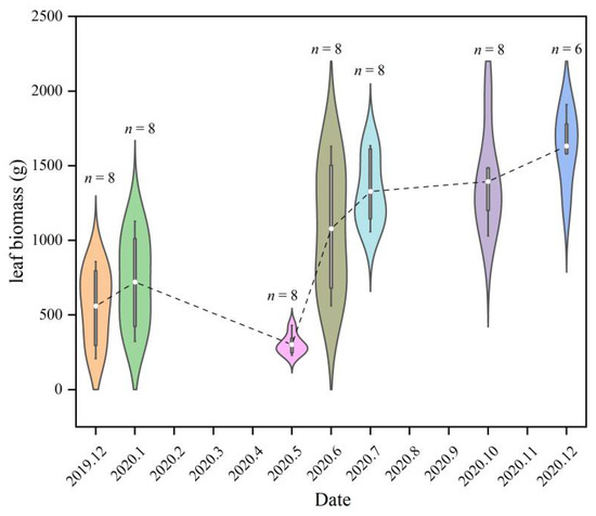
Figure 1.
Violin plots of the leaf biomass by month. The violin plot is an overlay of the kernel density plot in a mirror image on a box line plot, the n indicates the number of samples, with the white dots being the mean, the white box shape ranging from the lower to upper quartile, the thin black line indicating the whiskers, and the outer shape being the kernel density estimate.
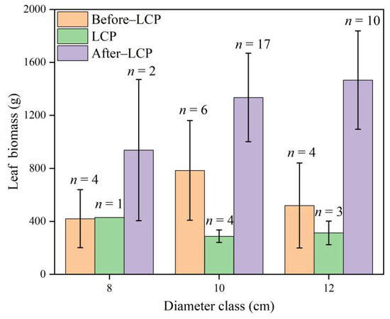
Figure 2.
Trends in the average of Moso bamboo leaf biomass in each diameter class for the three leaf change periods, n indicates the number of samples.
3.2. Correlation Analysis of the Leaf Biomass and Bamboo Measurement Factors
The results of the correlation analysis between the leaf biomass and the measured tree factors were significantly different for the two modeling strategies (Table 2). For the data from all months, leaf biomass was highly significantly correlated with crown length (p < 0.01), with a correlation coefficient of 0.356. For the three leaf change periods, leaf biomass in the Before-LCP was highly significantly correlated with culm height (p < 0.01) with a correlation coefficient of 0.657 and significantly correlated with age and crown length (p < 0.05), with correlation coefficients of 0.600 and 0.564, respectively. Leaf biomass in the LCP was significantly correlated with crown width (p < 0.05), with a correlation coefficient of 0.792. Leaf biomass in the After-LCP was highly significantly correlated with crown width and crown length (p < 0.01) with correlation coefficients of 0.576 and 0.495, respectively, followed by age (p < 0.05) with a correlation coefficient of −0.435. In general, crown length, crown width, and age were more highly correlated with leaf biomass, while diameter at breast height was not significantly correlated with leaf biomass. The descending order of correlation was as follows: crown length > crown width = age > culm height > diameter at breast height.
Table 2.
Results of correlation analysis between leaf biomass and bamboo measurement factors.
3.3. Statistical Model of Leaf Biomass
3.3.1. Leaf Biomass Model Based on Data from All Months (Model 1)
Multiple linear regressions with different combinations of independent variables were built for dataset from all months (Table A1). The combination of independent variables including A, D, CL, and CW was the best with small AIC and RMSEr values. The VIF value was 1.207, indicating that there was no collinearity problem for the selected multiple linear regression. The allometric models did not improve the accuracy of leaf biomass estimates (Table 3), which had higher AIC and RMSEr values than those of the selected multiple linear regression. Therefore, the multiple linear regression was used to estimate leaf biomass of Moso bamboo in this study.
Table 3.
Fitting results for allometric equations with diameter at breast height and culm height as independent variables.
Model 1 was constructed using the independent variables of A, D, CL, and CW. The multiple linear regression was as follows: W = −728.891 + 104.671A + 92.82D + 270.853CL − 163.289CW, with R2, RMSE, RMSEr, and AIC values of 0.228, 468.01 g, 46.79%, and 672.04, respectively. The R2, RMSE, and RMSEr values for the validation data were 0.108, 509.74 g, and 50.97%, respectively (Figure 3), using the leave-one-out cross-validation method. It can be seen that Model 1 has an R2 value less than 0.5 and an RMSEr value more than 45% for both fitted and validated data, indicating that Model 1 showed poor prediction accuracy. Therefore, Model 1 was not suitable for estimating Moso bamboo leaf biomass.
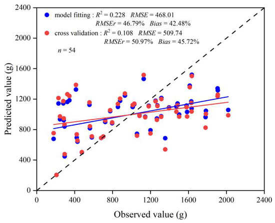
Figure 3.
Scatter plots of fitted and validated values for the leaf biomass model versus the measured values. Blue circles represent scatter plots of estimated leaf biomass versus measured leaf biomass, and red circles represent scatter plots of cross-validated leaf biomass versus measured leaf biomass. The red line represents the regression line between cross-validated leaf biomass and measured leaf biomass, the blue line represents the regression line between the fitted leaf biomass and measured leaf biomass, and the dashed line represents the 1:1 dashed line.
Model 1 line (Figure 3) show that there were significant deviations between the simulated and validated leaf biomass values and measured leaf biomass values. The sample points deviated significantly above and below the 1:1 line, indicating that most of the sample points were poorly fitted and predicted, with significant overestimation in low biomass areas and significant underestimation in high biomass areas.
In Figure 4, it can be seen that the residuals tend to increase with an increase in predicted leaf biomass, indicating that the residuals exist heteroscedasticity, which may overestimate or underestimate the variance of the parameter estimates, and thus, reduce the validity of the model for leaf biomass prediction.
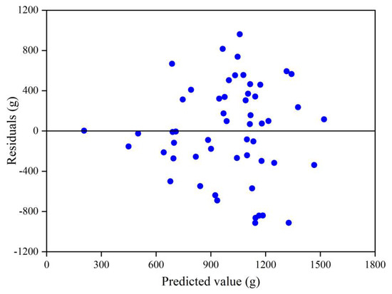
Figure 4.
Plot of residuals as a function of predicted values. Blue dots indicate residuals.
3.3.2. Leaf Biomass Model Based on Three Leaf Change Periods (Model 2)
The optimal independent variables for estimating leaf biomass of the three leaf change periods were determined based on AIC and RMSEr (Table A2, Table A3 and Table A4). The selected independent variables of the models and their fitting statistics for the Before-LCP, LCP, and After-LCP are summarized in Table 4. The leaf biomass model for the three leaf change periods passed the F-test and showed a high level of significance (p < 0.01). Their AIC values ranged from 58.77 to 334.70 and were smaller than those from Model 1. Their VIF values ranged from 1.63 to 2.07, indicating that there is no problem of multicollinearity. The model for the Before-LCP fitted, the R2 value was 0.784, and the RMSE and RMSEr values were 160.44 g and 24.19% (Table 4), respectively. The validated R2 value was 0.536, and the RMSE and RMSEr values were 243.38 g and 36.70% (Figure 5), respectively. The model for the LCP fitted R2 value reached 0.848, and the RMSE and RMSEr values were 27.06 g and 8.59%, respectively. The validated R2 value reached 0.474, and the RMSE and RMSEr values were 62.17 g and 19.73%, respectively. The model for the After-LCP fitted R2 value reached 0.583, and the RMSE and RMSEr values were 231.61 g and 17.00%, respectively. The validated R2 value reached 0.337, and the RMSE and RMSEr values were 295.02 g and 21.65%, respectively. The model for the LCP had the highest accuracy, followed by the Before-LCP, and the lowest accuracy was for the After-LCP. The fitted accuracy of the leaf biomass model based on the three leaf change periods with RMSEr values of less than 25.00% was significantly improved as compared with that of the leaf biomass model based on data from all months with an RMSEr value of 46.79%. From the plot of residuals as a function of predicted values (Figure 6), it can be seen that the residuals are more randomly distributed above and below the value of zero, indicating that the residuals are essentially without heteroskedasticity. Therefore, the model is valid for leaf biomass prediction.
Table 4.
The models for estimating leaf biomass of the three leaf change periods and their statistics.
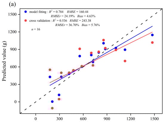
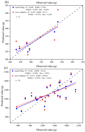
Figure 5.
Scatter plots of the fitted and validated values for the three leaf change periods versus the measured values: (a) Before-LCP; (b) LCP; (c) After-LCP. Blue circles represent scatter plots of estimated leaf biomass versus measured leaf biomass, and red circles represent scatter plots of cross-validated estimated leaf biomass versus measured leaf biomass. The red line represents the regression line between cross-validated estimated leaf biomass and measured leaf biomass, the blue line represents the regression line between estimated leaf biomass and measured leaf biomass, and the dashed line represents the 1:1 dashed line.
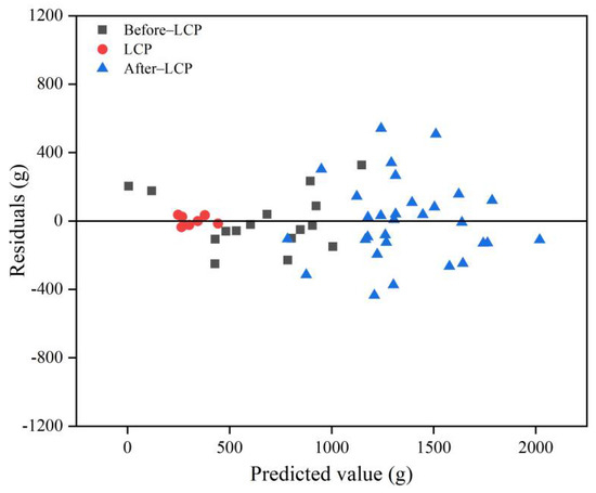
Figure 6.
Plot of residuals as a function of predicted values, black squares represent Before-LCP, red circles represent LCP, and blue triangles represent After-LCP.
The scatter plots between the estimated and measured values of leaf biomass from the different leaf change periods showed that the model fitted, and validated lines of the leaf biomass were close to the 1:1 line (Figure 5), indicating that the simulated and validated values of leaf biomass were consistent with the measured values. Relatively speaking, the errors in validation values in the After-LCP were higher than those in the other periods. Some of the samples deviated to a greater extent above and below the 1:1 line for the After-LCP, indicating that the predicted values of these samples had high error levels, and there was an obvious overestimation in the low biomass areas and an obvious underestimation in the high biomass areas.
3.4. Comparison Analysis of the Accuracy of the Two Modeling Strategies
The validated values of the 54 samples for Model 1 were calculated using the leave-one-out cross-validation. The validated values of the samples for each LCP of the Model 2 were also calculated using the leave-one-out cross-validation and there was a total of 54 validated values for Model 2. The accuracy of validated values for the 54 samples from both Model 1 and Model 2 were compared, and the results showed that there were significant differences in the accuracy statistics among the two modeling strategies (Table 5). The RMSE and RMSEr values of the leaf biomass model based on data from all months (Model 1) were 509.74 g and 50.97%, and the Bias and MAPE values were 45.72% and 72.86%, respectively. The RMSE and RMSEr values for the leaf biomass model based on the three leaf change periods (Model 2) were 242.40 g and 24.24%, and the Bias and MAPE values were 4.88% and 26.37%, respectively.
Table 5.
Accuracy evaluation indicators for the validated values for 54 samples from the models based on two different strategies.
The model prediction accuracies of the two modeling strategies differed significantly. The RMSE, RMSEr, Bias, and MAPE values from Model 1 were significantly higher than those of Model 2. Model 2 showed significantly lower values for RMSE, RMSEr, Bias, and MPAE, with a greater improvement in prediction accuracy than that in Model 1. This suggests that as the time span of the modeling samples used to build the model becomes shorter, it not only improves the model fit but also significantly improves the prediction accuracy.
Scatter plots between measured and estimated leaf biomass values for the two modeling schemes showed that the estimates from Model 1 deviated significantly from the 1:1 dashed line, and there was a large error in the estimates, thus, making it impossible to estimate the Moso bamboo leaf biomass with high accuracy (Figure 7a). The leaf biomass estimates from Model 1 were obviously overestimated for LCP (May) with an RMSEr value of 247.54% and Bias of 252.61%. As compared with the estimates of Model 1, the estimates from Model 2 were less discrete and more evenly distributed on both sides of the 1:1 dashed line, and the prediction accuracy of Model 2 was greatly improved (Figure 7b). There was no obvious underestimation or overestimation of the leaf biomass estimates (Figure 7b). Therefore, the estimates of leaf biomass from Model 2 were very close to the measured values and more accurate than those from Model 1.
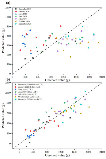
Figure 7.
Scatter plots of predicted versus measured leaf biomass levels for the two scenarios: (a) Model 1; (b) Model 2. Black squares represent scatter plots of estimated versus measured leaf biomass in December 2019; red circles represent scatter plots of estimated versus measured leaf biomass in January 2020; dark blue triangles represent scatter plots of estimated versus measured leaf biomass in May 2020; green triangles represent scatter plots of estimated and measured leaf biomass in June 2020; purple diamonds represent scatter plots of estimated and measured leaf biomass in July 2020; yellow triangles represent scatter plots of estimated and measured leaf biomass in October 2020; blue triangles represent scatter plots of estimated and measured leaf biomass in December 2020; dashed lines represent the 1:1 dashed line.
4. Discussion
4.1. Temporal Variations in the Leaf Biomass of the Moso Bamboo
The results of the study showed that the leaf biomass of the Moso bamboo in the off-year varied significantly with time, with a decreasing trend from January to May, reaching its lowest value in May, followed by an increasing trend from June to December. This is mainly due to the physiological characteristics of the leaf changes in off-years. The old leaves turn yellow from January to March and start to drop and are replaced by new leaves from April to May, which results in a gradual decrease in leaf biomass. New leaves finish their growth and development from June to August, with a gradual increase in leaf biomass [31,41,45].
4.2. Correlation Analysis of the Leaf Biomass and Bamboo Measurement Factors
In terms of the degree of relationship with leaf biomass, crown length was the highest, followed by crown width, age, culm height, and diameter at breast height. Canopy is an important site of plant photosynthetic processes [53], and canopy size is an important parameter of canopy structure that affects the exchange of energy and materials between forest ecosystems and the atmosphere, as well as the production of trees and the distribution of production among organs [53,54]; crown width and length are commonly used as indicators to measure canopy size horizontally and vertically, and they are closely related to leaf biomass [6,55]. Previous studies have found that the accuracy of leaf biomass estimates was not high using the variables of diameter at breast height and tree height, while the accuracy increased after considering crown width and crown length into the models [14,56,57,58,59]. In this study, a high correlation was observed between crown length and crown width and Moso bamboo leaf biomass, and this has an important influence on Moso bamboo leaf biomass estimation. Therefore, the inclusion of variables related to canopy structure in the model, such as crown width and crown length, can help to improve the accuracy of leaf biomass estimation [4,23,60].
Age as a factor has an impact on plant biomass estimations, as it is a potential source of error in ecosystem biomass and nutrient stock predictions and is often overlooked [61]. Significant differences were found in the leaf biomass of Moso bamboo at different ages. In this study (Figure A1), the leaf biomass of Moso bamboo for the 8 cm and 12 cm diameter classes increased as age increased, which is consistent with the results of several previous studies [62,63,64]. The leaf biomass of Moso bamboo for the 10 cm diameter class increased with age, and then decreased, with the maximum leaf biomass at 2 du, which was consistent with the findings of Zhu et al. [65]. Differences in age can lead to differences in leaf biomass and also in Moso bamboo pole biomass, total aboveground biomass, belowground root biomass, and total biomass per plant [66]. Therefore, leaf biomass has a wide range of fluctuations among the Moso bamboo individuals of different ages, and predictions of leaf biomass using the anisotropic growth equation without considering the age factor will lead to large errors in the prediction results [67].
The diameter at breast height is a common factor used to fit biomass models. It is not feasible to estimate Moso bamboo leaf biomass using a single diameter at breast height factor, and the accuracy of the model driven by diameter at breast height is poor [59]. Therefore, most scholars generally combine diameter at breast height with other bamboo measurement factors, such as culm height [68], age [69], and clear bole height [70], as it improves the Moso bamboo leaf biomass estimation accuracy. The shoots of Moso bamboo in this study were cut, which largely reduced their differences in height. The larger the diameter at breast height and the taller of Moso bamboo, the more leaf biomass was removed by shoot cutting [71], which reduced the differences in leaf biomass between those with a large culm height and diameter at breast height and those with a small culm height and diameter at breast height. This may be the main reason for the low correlations between the diameter at breast height and culm height and leaf biomass of the Moso bamboo. In most cases, the variability in above-ground biomass is mainly explained by variability in diameter at breast height [72], and the range of diameter at breast height of sample bamboos has an important influence on the feasible of the leaf biomass model. In this study, most of sample bamboos were selected at 10 cm and 12 cm diameter classes, which may be one of the reasons for the low correlation between leaf biomass and diameter at breast height. Attention should be paid to predict leaf biomass of Moso bamboo with diameter at breast height less than 7.0 cm using the models proposed in this study.
4.3. Factors Affecting the Accuracy of the Model
The growth of Moso bamboo differs from that of other tree species, and it has a distinct growth pattern. It takes approximately two months for Moso bamboo to grow from shoot to mature bamboo, and after this, the diameter at breast height and the culm height no not change [26,33,73]. The crown length and width increase with the growth of the diameter at breast height and bamboo height, and then they also stop changing [74]. As old leaves fall off and new leaves grow between April and May in the off-year of Moso bamboo [43], its leaf biomass can change significantly, but the tree measurements do not change. Thus, the dispersion between Moso bamboo leaf biomass and the bamboo measurement factors increases and their correlation decreases; therefore, the model established based on the sample data from all months (Model 1) had low accuracy. The model constructed by segmenting the entire leaf change process into three periods (Model 2) significantly improved the correlation between leaf biomass and bamboo measurement factors and increased the model prediction accuracy. To obtain high accuracy of leaf area index estimates, leaf area index inversion models were established in the jointing, booting, and heading stages for winter wheat, and they achieved good performance and high accuracy with R2 and RMSE values of 0.918 and 0.675, respectively [75].
The shoot cutting measure has a strong influence on the correlations between diameter at breast height and culm height and the leaf biomass of Moso bamboo; therefore, the leaf biomass models in this study are only suitable for Moso bamboo with shoot cutting measures. In this study, leaf biomass data for the key months of Moso bamboo leaf change (February, March, and April) were not available; therefore, further data are required in future studies to evaluate the feasibility and prediction accuracy of the leaf biomass models. Many studies have shown that stand quality, elevation, and stand density affect Moso bamboo leaf biomass; therefore, these abiotic factors can be added to prediction models in future studies to improve the prediction accuracy of the models and also to expand their applicability and generalization to large-scale areas [76].
5. Conclusions
The leaf biomass of the Moso bamboo significantly decreased in the off-year from March–May when the leaf changes occurred and increased significantly from June–August when the new leaf growth and development were completed. To estimate the leaf biomass more accurately, two modeling strategies based on data from the whole year and three leaf change periods were compared. Crown length, crown width, and age were useful independent variables for the estimation of the leaf biomass of Moso bamboo. The comparative analysis of the results from the two modeling strategies showed that a better fit and higher prediction accuracy were achieved with the model that used data for three leaf change periods, as the R2 value was in the range of 0.583–0.848, and the prediction error was in the range of 8.59–24.19%. The model with a worse performance was based on the data from all months, as the R2 value was 0.228, and the prediction error was 46.79%. This further showed that the leaf biomass varied significantly among the leaf change periods, and that it was not possible to construct a general estimation model for leaf biomass over a whole year. This study explores the dynamic changes in Moso bamboo leaf biomass during leaf changes and provides reference data and technical support for the development of models and protocols for accurate leaf biomass estimation. This study also has shortcomings, as only biotic factors were considered, and no abiotic factors were assessed as independent variables, making the application of the models somewhat limited. More sample data should be used to validate the applicability and generalization of the models in future studies.
Author Contributions
Conceptualization, X.X. and Z.Z.; methodology, Z.Z.; validation, Z.Z.; formal analysis, X.X. and Z.Z.; investigation, X.X., Z.Z, Y.T., J.W., H.X. and L.H.; data curation, X.X., Z.Z., Y.T., J.W., H.X., L.H. and Y.T.; writing—original draft preparation, Z.Z.; writing—review and editing, X.X.; supervision, X.X; funding acquisition, X.X. All authors have read and agreed to the published version of the manuscript.
Funding
This research was supported by the National Natural Science Foundation of China (grant no. 31870619) and the Natural Science Foundation of Zhejiang Province (grant no. LY21C030001).
Institutional Review Board Statement
Not applicable.
Informed Consent Statement
Not applicable.
Data Availability Statement
The authors confirm that the data supporting the findings of this study are available within the article. Raw data supporting the findings of this study are available from the corresponding authors on request.
Conflicts of Interest
The authors declare no conflict of interest.
Appendix A
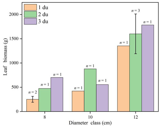
Figure A1.
Trends in average of leaf biomass at different ages for each diameter class. Yellow represents 1 du Moso bamboo, green represents 2 du Moso bamboo, and purple represents 3 du Moso bamboo. Sample data for 8 cm diameter class was from December 2019, Sample data for 10 cm diameter class was from January 2020, and Sample data for 12 cm diameter class was from October 2020.
Table A1.
Fitting results of multiple linear regression models with different combination of independent variables for the Model 1.
Table A1.
Fitting results of multiple linear regression models with different combination of independent variables for the Model 1.
| Model Variables | AIC | R2 | RMSE (g) | RMSEr (%) | VIF |
|---|---|---|---|---|---|
| D, CL | 670.35 | 0.194 | 483.57 | 48.35 | 1.001 |
| A, D, CL | 670.71 | 0.218 | 470.93 | 47.09 | 1.010 |
| D, CL, CW | 671.16 | 0.211 | 472.94 | 47.29 | 1.140 |
| A, D, CL, CW | 672.04 | 0.228 | 468.01 | 46.79 | 1.207 |
| A, D, H, CL | 672.04 | 0.228 | 468.01 | 46.79 | 2.675 |
| D, H, CL | 672.27 | 0.195 | 477.78 | 47.77 | 2.313 |
| CL, CW | 672.47 | 0.162 | 487.64 | 48.76 | 1.083 |
| CL | 672.67 | 0.127 | 497.64 | 49.76 | 1.000 |
| D, H, CL, CW | 672.86 | 0.216 | 471.60 | 47.15 | 2.444 |
| H, CL | 672.87 | 0.155 | 489.42 | 48.93 | 1.040 |
| A, D, H, CL, CW | 673.09 | 0.241 | 463.94 | 46.39 | 2.745 |
| A, CL | 673.56 | 0.144 | 492.58 | 49.25 | 1.003 |
| H, CL, CW | 673.59 | 0.175 | 483.69 | 48.36 | 1.204 |
| A, CL, CW | 673.87 | 0.171 | 484.92 | 48.48 | 1.133 |
| A, H, CL | 674.18 | 0.166 | 486.29 | 48.62 | 1.076 |
| A, H, CL, CW | 675.15 | 0.182 | 481.71 | 48.16 | 1.236 |
| D | 675.98 | 0.072 | 513.16 | 51.31 | 1.000 |
| A, D | 676.87 | 0.090 | 507.92 | 50.78 | 1.007 |
| H | 676.91 | 0.055 | 517.56 | 51.75 | 1.000 |
| D, H | 677.78 | 0.075 | 512.22 | 51.21 | 2.155 |
| D, CW | 677.94 | 0.072 | 512.98 | 51.29 | 1.045 |
| A, H | 678.58 | 0.061 | 516.01 | 51.59 | 1.030 |
| A, D, H | 678.87 | 0.091 | 507.88 | 50.78 | 2.439 |
| A, D, CW | 678.87 | 0.090 | 507.90 | 50.78 | 1.109 |
| H, CW | 678.87 | 0.056 | 517.41 | 51.73 | 1.064 |
| A | 679.28 | 0.013 | 529.05 | 52.90 | 1.000 |
| CW | 679.63 | 0.007 | 530.82 | 53.07 | 1.000 |
| D, H, CW | 679.77 | 0.075 | 512.13 | 51.20 | 2.197 |
| A, H, CW | 680.57 | 0.061 | 515.98 | 51.59 | 1.100 |
| A, D, H, CW | 680.86 | 0.091 | 507.86 | 50.78 | 2.448 |
| A, CW | 681.10 | 0.016 | 528.18 | 52.81 | 1.049 |
Note: A denotes age; D denotes diameter at breast height; H denotes culm height; CL denotes crown length; CW denotes crown width.
Table A2.
Fitting results of multiple linear regression models with different combination of independent variable for the Before-LCP of Model 2.
Table A2.
Fitting results of multiple linear regression models with different combination of independent variable for the Before-LCP of Model 2.
| Model Variables | AIC | R2 | RMSE (g) | RMSEr (%) | VIF |
|---|---|---|---|---|---|
| A, H, CW | 170.25 | 0.759 | 169.51 | 25.56 | 1.085 |
| A, H, CL, CW | 170.49 | 0.784 | 160.44 | 24.19 | 1.916 |
| A, D, H, CW | 171.77 | 0.766 | 166.94 | 25.18 | 5.160 |
| A, D, CL, CW | 172.26 | 0.759 | 168.56 | 25.57 | 1.253 |
| A, D, H, CL, CW | 172.47 | 0.784 | 160.33 | 24.18 | 9.160 |
| A, H, CL | 174.48 | 0.686 | 193.43 | 29.17 | 1.815 |
| A, CL, CW | 174.57 | 0.684 | 193.97 | 29.25 | 1.017 |
| A, D, CL | 174.57 | 0.684 | 194.01 | 29.26 | 1.233 |
| A, H | 175.03 | 0.632 | 209.49 | 31.59 | 1.070 |
| A, CL | 175.39 | 0.623 | 211.88 | 31.95 | 1.008 |
| A, D, CW | 175.93 | 0.656 | 202.43 | 30.53 | 1.003 |
| D, H, CW | 176.30 | 0.648 | 204.77 | 30.88 | 3.858 |
| A, D, H, CL | 176.33 | 0.689 | 192.53 | 29.03 | 8.312 |
| A, D, H | 176.95 | 0.633 | 208.95 | 31.51 | 5.036 |
| H, CW | 177.22 | 0.577 | 224.35 | 33.83 | 1.011 |
| A, D | 178.02 | 0.556 | 230.02 | 34.69 | 1.000 |
| D, H, CL, CW | 178.28 | 0.648 | 204.65 | 30.86 | 6.224 |
| H, CL, CW | 178.77 | 0.589 | 221.20 | 33.36 | 1.776 |
| H | 179.96 | 0.432 | 260.14 | 39.23 | 1.000 |
| D, H | 180.32 | 0.487 | 247.18 | 37.27 | 3.802 |
| H, CL | 180.94 | 0.467 | 251.99 | 38.00 | 1.692 |
| A, CW | 181.53 | 0.447 | 256.66 | 38.70 | 1.001 |
| A | 181.85 | 0.361 | 275.97 | 41.62 | 1.000 |
| D, H, CL | 181.87 | 0.501 | 243.71 | 36.75 | 5.845 |
| CL | 182.87 | 0.318 | 284.93 | 42.97 | 1.000 |
| CL, CW | 183.23 | 0.385 | 270.69 | 40.82 | 1.009 |
| D, CL, CW | 183.48 | 0.448 | 256.31 | 38.65 | 1.241 |
| D, CL | 183.64 | 0.369 | 274.15 | 41.34 | 1.221 |
| D, CW | 185.12 | 0.308 | 287.14 | 43.30 | 1.003 |
| D | 185.50 | 0.197 | 309.30 | 46.64 | 1.000 |
| CW | 187.38 | 0.096 | 328.06 | 49.47 | 1.000 |
Note: A denotes age; D denotes diameter at breast height; H denotes culm height; CL denotes crown length; CW denotes crown width.
Table A3.
Fitting results of multiple linear regression models with different combination of independent variable for the LCP of Model 2.
Table A3.
Fitting results of multiple linear regression models with different combination of independent variable for the LCP of Model 2.
| Model Variables | AIC | R2 | RMSE (g) | RMSEr (%) | VIF |
|---|---|---|---|---|---|
| A, CW | 56.98 | 0.844 | 27.42 | 8.70 | 1.262 |
| A, D, CW | 58.67 | 0.850 | 26.90 | 8.53 | 1.794 |
| A, CL, CW | 58.77 | 0.848 | 27.06 | 8.59 | 1.629 |
| A, H, CW | 58.98 | 0.844 | 27.41 | 8.70 | 1.373 |
| A, D, H, CW | 60.28 | 0.857 | 26.24 | 8.32 | 3.688 |
| A, D, CL, CW | 60.46 | 0.854 | 26.55 | 8.42 | 1.847 |
| A, H, CL, CW | 60.74 | 0.848 | 27.02 | 8.57 | 1.869 |
| CW | 61.94 | 0.627 | 42.37 | 13.44 | 1.000 |
| CL, CW | 62.11 | 0.704 | 37.77 | 11.98 | 1.002 |
| A, D, H, CL, CW | 62.22 | 0.858 | 26.15 | 8.30 | 4.148 |
| H, CL, CW | 63.41 | 0.729 | 36.16 | 11.47 | 1.109 |
| H, CW | 63.52 | 0.647 | 41.26 | 13.09 | 1.104 |
| D, CW | 63.84 | 0.632 | 42.10 | 13.36 | 1.289 |
| D, CL, CW | 64.08 | 0.705 | 37.71 | 11.96 | 1.312 |
| D, H, CL, CW | 64.52 | 0.757 | 34.21 | 10.85 | 2.166 |
| D, H, CW | 64.55 | 0.687 | 38.83 | 12.32 | 2.137 |
| D | 68.15 | 0.190 | 62.47 | 19.82 | 1.000 |
| CL | 69.37 | 0.057 | 67.40 | 21.39 | 1.000 |
| D, H | 69.53 | 0.251 | 60.08 | 19.06 | 1.829 |
| H | 69.74 | 0.012 | 68.98 | 21.88 | 1.000 |
| D, CL | 69.76 | 0.229 | 60.93 | 19.33 | 1.009 |
| A | 69.82 | 0.003 | 69.31 | 21.99 | 1.000 |
| A, D | 70.14 | 0.192 | 62.40 | 19.80 | 1.001 |
| D, H, CL | 71.12 | 0.288 | 58.56 | 18.58 | 1.842 |
| H, CL | 71.29 | 0.067 | 67.05 | 21.27 | 1.002 |
| A, CL | 71.34 | 0.060 | 67.28 | 21.35 | 1.244 |
| A, D, H | 71.41 | 0.262 | 59.64 | 18.92 | 2.562 |
| A, H | 71.65 | 0.023 | 68.61 | 21.77 | 1.169 |
| A, D, CL | 71.73 | 0.232 | 60.83 | 19.30 | 1.255 |
| A, D, H, CL | 72.46 | 0.345 | 56.19 | 17.83 | 2.792 |
| A, H, CL | 73.28 | 0.067 | 67.04 | 21.27 | 1.558 |
Note: A denotes age; D denotes diameter at breast height; H denotes culm height; CL denotes crown length; CW denotes crown width.
Table A4.
Fitting results of multiple linear regression models with different combination of independent variable for the After-LCP of Model 2.
Table A4.
Fitting results of multiple linear regression models with different combination of independent variable for the After-LCP of Model 2.
| Model Variables | AIC | R2 | RMSE (g) | RMSEr (%) | VIF |
|---|---|---|---|---|---|
| A, D, CW | 334.00 | 0.565 | 236.65 | 17.37 | 1.177 |
| D, CW | 334.51 | 0.527 | 246.77 | 18.11 | 1.062 |
| A, D, CL, CW | 334.70 | 0.583 | 231.61 | 17.00 | 2.074 |
| A, D, H, CW | 335.98 | 0.565 | 236.61 | 17.36 | 1.655 |
| D, H, CL, CW | 336.36 | 0.559 | 238.09 | 17.47 | 2.214 |
| D, H, CW | 336.46 | 0.527 | 246.56 | 18.09 | 1.546 |
| D, CL, CW | 336.46 | 0.554 | 239.37 | 17.57 | 2.019 |
| A, D, H, CL, CW | 336.53 | 0.585 | 230.96 | 16.95 | 2.220 |
| A, CW | 339.77 | 0.436 | 269.37 | 19.77 | 1.044 |
| A, H, CW | 339.95 | 0.469 | 261.36 | 19.18 | 1.153 |
| A, D, CL | 340.41 | 0.461 | 263.34 | 19.33 | 1.182 |
| D, CL | 340.61 | 0.420 | 273.19 | 20.05 | 1.058 |
| A, D, H, CL | 341.19 | 0.482 | 258.06 | 18.94 | 1.765 |
| A, CL, CW | 341.40 | 0.443 | 267.73 | 19.65 | 2.032 |
| A, H, CL, CW | 341.75 | 0.472 | 260.48 | 19.12 | 2.213 |
| H, CW | 342.72 | 0.377 | 282.98 | 20.77 | 1.094 |
| CW | 342.87 | 0.331 | 293.28 | 21.52 | 1.000 |
| A, CL | 343.93 | 0.352 | 288.75 | 21.19 | 1.060 |
| CL, CW | 344.15 | 0.347 | 289.79 | 21.27 | 1.995 |
| D, H, CL | 344.27 | 0.450 | 265.92 | 19.52 | 2.200 |
| H, CL, CW | 344.27 | 0.387 | 280.87 | 20.61 | 2.200 |
| A, H, CL | 345.70 | 0.357 | 287.64 | 21.11 | 1.077 |
| CL | 346.49 | 0.245 | 311.52 | 22.86 | 1.000 |
| H, CL | 348.15 | 0.254 | 309.77 | 22.73 | 1.012 |
| A | 348.65 | 0.189 | 322.95 | 23.70 | 1.000 |
| A, D | 349.31 | 0.224 | 315.82 | 23.18 | 1.065 |
| A, H | 350.63 | 0.189 | 322.87 | 23.70 | 1.001 |
| A, D, H | 350.84 | 0.236 | 313.37 | 23.00 | 1.609 |
| D | 352.30 | 0.084 | 343.22 | 25.19 | 1.000 |
| D, H | 353.48 | 0.109 | 338.55 | 24.85 | 1.487 |
| H | 354.90 | 0.001 | 358.38 | 26.30 | 1.000 |
Note: A denotes age; D denotes diameter at breast height; H denotes culm height; CL denotes crown length; CW denotes crown width.
References
- Wahyuningrum, N. Foliage Biomass Estimation in Tropical Logged over Forest East Kalimantan, Indonesia. Master’s Thesis, University of Twente, Enschede, The Netherlands, 2005. [Google Scholar]
- Wang, Y.P.; Jarvis, P.G. Description and validation of an array model-MAESTRO. Agric. For. Meteorol. 1990, 51, 257–280. [Google Scholar] [CrossRef]
- Gillespie, A.R.; Allen, H.L.; Vose, J.M. Amount and vertical distribution of foliage of young loblolly pine trees as affected by canopy position and silvicultural treatment. Can. J. For. Res. 1994, 24, 1337–1344. [Google Scholar] [CrossRef]
- Clough, B.J.; Russell, M.B.; Domke, G.M.; Woodall, C.W.; Radtke, P.J. Comparing tree foliage biomass models fitted to a multispecies, felled-tree biomass dataset for the United States. Ecol. Modell. 2016, 333, 79–91. [Google Scholar] [CrossRef] [Green Version]
- Dougherty, P.M.; Hennessey, T.C.; Zarnoch, S.J.; Stenberg, P.T.; Holeman, R.T.; Wittwer, R.F. Effects of stand development and weather on monthly leaf biomass dynamics of a loblolly pine (Pinus taeda L.) stand. For. Ecol. Manag. 1995, 72, 213–227. [Google Scholar] [CrossRef]
- Goudie, J.W.; Parish, R.; Antos, J.A. Foliage biomass and specific leaf area equations at the branch, annual shoot and whole-tree levels for lodgepole pine and white spruce in British Columbia. For. Ecol. Manag. 2016, 361, 286–297. [Google Scholar] [CrossRef]
- Socha, J.; Wezyk, P. Allometric equations for estimating the foliage biomass of Scots pine. Eur. J. For. Res. 2007, 126, 263–270. [Google Scholar] [CrossRef]
- Di Cosmo, L.; Gasparini, P.; Tabacchi, G. A national-scale, stand-level model to predict total above-ground tree biomass from growing stock volume. For. Ecol. Manag. 2016, 361, 269–276. [Google Scholar] [CrossRef]
- Sytnyk, S.; Lovynska, V.; Lakyda, I. Foliage biomass qualitative indices of selected forest forming tree species in Ukrainian steppe. Folia Oecologica. 2017, 44, 38–45. [Google Scholar] [CrossRef] [Green Version]
- Amthor, J.S. Scaling CO2-photosynthesis relationships from the leaf to the canopy. Photosynth. Res. 1994, 39, 321–350. [Google Scholar] [CrossRef]
- Tatsuhara, S.; Kurashige, H. Estimating foliage biomass in a natural deciduous broad-leaved forest area in a mountainous district. For. Ecol. Manag. 2001, 152, 141–148. [Google Scholar] [CrossRef]
- Kaushal, R.; Subbulakshmi, V.; Tomar, J.M.S.; Alam, N.M.; Jayaparkash, J.; Mehta, H.; Chaturvedi, O.P. Predictive models for biomass and carbon stock estimation in male bamboo (Dendrocalamus strictus L.) in Doon valley, India. Acta Ecol. Sin. 2016, 36, 469–476. [Google Scholar] [CrossRef]
- Fu, W.; Wu, Y. Estimation of aboveground biomass of different mangrove trees based on canopy diameter and tree height. Procedia Environ. Sci. 2011, 10, 2189–2194. [Google Scholar] [CrossRef] [Green Version]
- Jelonek, T.; Pazdrowski, W.; Walkowiak, R.; Arasimowicz-Jelonek, M.; Tomczak, A. Allometric models of foliage biomass in scots pine (Pinus sylvestris L.). Polish J. Environ. Stud. 2011, 20, 355–364. [Google Scholar]
- Dong, L.; Zhang, L.; Li, F. Developing two additive biomass equations for three coniferous plantation species in northeast China. Forests 2016, 7, 136. [Google Scholar] [CrossRef] [Green Version]
- Zhu, X.; Liu, D. Improving forest aboveground biomass estimation using seasonal Landsat NDVI time-series. ISPRS J. Photogramm. Remote Sens. 2015, 102, 222–231. [Google Scholar] [CrossRef]
- Shen, W.; Li, M.; Huang, C.; Wei, A. Quantifying Live Aboveground Biomass and Forest Disturbance of Mountainous Natural and Plantation Forests in Northern Guangdong, China, Based on Multi-Temporal Landsat, PALSAR and Field Plot Data. Remote Sens. 2016, 8, 595. [Google Scholar] [CrossRef] [Green Version]
- Wang, Y.; Zhang, X.; Guo, Z. Estimation of tree height and aboveground biomass of coniferous forests in North China using stereo ZY-3, multispectral Sentinel-2, and DEM data. Ecol. Indic. 2021, 126, 107645. [Google Scholar] [CrossRef]
- Gower, S.T.; Kucharik, C.J.; Norman, J.M. Direct and indirect estimation of leaf area index, f(APAR), and net primary production of terrestrial ecosystems. Remote Sens. Environ. 1999, 70, 29–51. [Google Scholar] [CrossRef]
- Seidel, D.; Fleck, S.; Leuschner, C.; Hammett, T. Review of ground-based methods to measure the distribution of biomass in forest canopies. Ann. For. Sci. 2011, 68, 225–244. [Google Scholar] [CrossRef] [Green Version]
- Kumar, L.; Sinha, P.; Taylor, S.; Alqurashi, A.F. Review of the use of remote sensing for biomass estimation to support renewable energy generation. J. Appl. Remote Sens. 2015, 9, 097696. [Google Scholar] [CrossRef]
- Kittredge, J. Estimation of the Amount of Foliage of Trees and Stands. J. For. 1944, 42, 905–912. [Google Scholar] [CrossRef]
- Temesgen, H.; Monleon, V.; Weiskittel, A.; Wilson, D. Sampling strategies for efficient estimation of tree foliage biomass. For. Sci. 2011, 57, 153–163. [Google Scholar] [CrossRef]
- Cleary, M.B.; Naithani, K.J.; Ewers, B.E.; Pendall, E. Upscaling CO2 fluxes using leaf, soil and chamber measurements across successional growth stages in a sagebrush steppe ecosystem. J. Arid. Environ. 2015, 121, 43–51. [Google Scholar] [CrossRef]
- Ross, J.; Ross, V.; Koppel, A. Estimation of leaf area and its vertical distribution during growth period. Agric. For. Meteorol. 2000, 101, 237–246. [Google Scholar] [CrossRef]
- Song, X.; Peng, C.; Zhou, G.; Gu, H.; Li, Q.; Zhang, C. Dynamic allocation and transfer of non-structural carbohydrates, a possible mechanism for the explosive growth of Moso bamboo (Phyllostachys heterocycla). Sci. Rep. 2016, 6, 25908. [Google Scholar] [CrossRef] [PubMed]
- Zhou, G.; Jiang, P. Density, Storage and Spatial Distribution of Carbon in Phyllostachy pubescens Forest. Sci. Silvae Sin. 2004, 40, 20–24. [Google Scholar] [CrossRef]
- Komatsu, H.; Onozawa, Y.; Kume, T.; Tsuruta, K.; Kumagai, T.; Shinohara, Y.; Otsuki, K. Stand-scale transpiration estimates in a Moso bamboo forest: II. Comparison with coniferous forests. For. Ecol. Manag. 2010, 260, 1295–1302. [Google Scholar] [CrossRef]
- Yen, T.M.; Lee, J.S. Comparing aboveground carbon sequestration between moso bamboo (Phyllostachys heterocycla) and China fir (Cunninghamia lanceolata) forests based on the allometric model. For. Ecol. Manag. 2011, 261, 995–1002. [Google Scholar] [CrossRef]
- Yen, T.M. Culm height development, biomass accumulation and carbon storage in an initial growth stage for a fast-growing moso bamboo (Phyllostachy pubescens). Bot. Stud. 2016, 57, 10. [Google Scholar] [CrossRef] [Green Version]
- Song, X.; Chen, X.; Zhou, G.; Jiang, H.; Peng, C. Observed high and persistent carbon uptake by Moso bamboo forests and its response to environmental drivers. Agric. For. Meteorol. 2017, 247, 467–475. [Google Scholar] [CrossRef]
- Liu, Y.H.; Yen, T.M. Assessing aboveground carbon storage capacity in bamboo plantations with various species related to its affecting factors across Taiwan. For. Ecol. Manag. 2021, 481, 118745. [Google Scholar] [CrossRef]
- Zhou, G.M.; Jiang, P.K.; Xu, Q.F. Carbon Fixing and Transition in the Ecosystem of Bamboo Stands, 1st ed.; Science Press: Beijing, China, 2010; p. 6. [Google Scholar]
- Kleinhenz, V.; Midmore, D.J. Aspects of bamboo agronomy. Advan Agron. 2001, 74, 99–153. [Google Scholar]
- Lu, G.F.; Zhou, G.M.; Gu, C.Y.; Shang, Z.Z. Dynamic change of Phyllostachys edulis forest canopy parameters and their relationships with photosynthetic active radiation in the bamboo shooting growth phase. J. Zhejiang A F Univ. 2012, 26, 844–850. (In Chinese) [Google Scholar] [CrossRef]
- Xu, X.; Du, H.; Zhou, G.; Mao, F.; Li, X.; Zhu, D.; Li, Y.; Cui, L. Remote estimation of canopy leaf area index and chlorophyll content in Moso bamboo (Phyllostachys edulis (Carrière) J. Houz.) forest using MODIS reflectance data. Ann. For. Sci. 2018, 75, 33. [Google Scholar] [CrossRef] [Green Version]
- Gui, R.Y.; Shao, J.F.; Yu, Y.M.; Zhu, Y.J.; Dong, D.Y. Influence of Obtruncation on Physical and Mechanical Properties of 5 Years Old Culms of Phyllostachys edulis. Acta Agric. Univ. Jiangxiensis 2011, 37, 6–10. (In Chinese) [Google Scholar] [CrossRef]
- Zhu, Q.G.; Jin, A.W.; Wang, Y.K.; Qiu, Y.H.; Li, X.T.; Zhang, S.H. Biomass allocation of branches and leaves in Phyllostachys heterocycla ‘Pubescens’ under different management modes: Allometric scaling analysis. Chinese J. Plant Ecol. 2014, 37, 811–819. (In Chinese) [Google Scholar] [CrossRef]
- Mao, F.; Li, P.; Zhou, G.; Du, H.; Xu, X.; Shi, Y.; Mo, L.; Zhou, Y.; Tu, G. Development of the BIOME-BGC model for the simulation of managed Moso bamboo forest ecosystems. J. Environ. Manag. 2016, 172, 29–39. [Google Scholar] [CrossRef]
- Zhang, S.S.; Ding, X.C.; Zhang, Z.Y.; Cai, H.J. Effects of Pruning Hormonal and Single-Sugar Regulation by Hooking Shooting on the Yield of Dendracalamus latiforus. Sci. Silvae Sin. 2018, 54, 31–39. (In Chinese) [Google Scholar] [CrossRef]
- Shang, Z.Z.; Zhou, G.M.; Du, H.Q. Relationship between above-ground biomass and DBH for Phyllostachys edulis stands based on fractal theory. J. Zhejiang A F Univ. 2013, 30, 319–324. (In Chinese) [Google Scholar] [CrossRef]
- Zhou, Y.; Zhou, G.; Du, H.; Shi, Y.; Mao, F.; Liu, Y.; Xu, L.; Li, X.; Xu, X. Biotic and abiotic influences on monthly variation in carbon fluxes in on-year and off-year Moso bamboo forest. Trees-Struct. Funct. 2019, 33, 153–169. [Google Scholar] [CrossRef]
- Xu, X.; Zhou, G.; Liu, S.; Du, H.; Mo, L.; Shi, Y.; Jiang, H.; Zhou, Y.; Liu, E. Implications of ice storm damages on the water and carbon cycle of bamboo forests in southeastern China. Agric. For. Meteorol. 2013, 177, 35–45. [Google Scholar] [CrossRef]
- Du, H.; Zhou, G.; Fan, W.; Ge, H.; Xu, X.; Shi, Y.; Fan, W. Spatial heterogeneity and carbon contribution of aboveground biomass of moso bamboo by using geostatistical theory. Plant Ecol. 2010, 207, 131–139. [Google Scholar] [CrossRef]
- Li, X.; Du, H.; Zhou, G.; Mao, F.; Zhang, M.; Han, N.; Fan, W.; Liu, H.; Huang, Z.; He, S.; et al. Phenology estimation of subtropical bamboo forests based on assimilated MODIS LAI time series data. ISPRS J. Photogramm. Remote Sens. 2021, 173, 262–277. [Google Scholar] [CrossRef]
- Shahabedini, S.; Ghahramany, L.; Pulido, F.; Khosravi, S.; Moreno, G. Estimating leaf biomass of pollarded lebanon oak in open silvopastoral systems using allometric equations. Trees 2018, 32, 99–108. [Google Scholar] [CrossRef]
- Shi, G.; Zhou, Y.; Sang, Y.; Huang, H.; Zhang, J.; Meng, P.; Cai, L. Modeling the response of negative air ions to environmental factors using multiple linear regression and random forest. Ecol. Inform. 2021, 66, 101464. [Google Scholar] [CrossRef]
- Isagi, Y.; Kawahara, T.; Kamo, K.; Ito, H. Net production and carbon cycling in a bamboo Phyllostachys pubesces stand. Plant Ecol. 1997, 130, 41–52. [Google Scholar] [CrossRef]
- Xu, Z.; Du, W.; Zhou, G.; Qin, L.; Meng, S.; Yu, J.; Sun, Z.; SiQing, B.; Liu, Q. Aboveground biomass allocation and additive allometric models of fifteen tree species in northeast China based on improved investigation methods. For. Ecol. Manag. 2022, 505, 119918. [Google Scholar] [CrossRef]
- Burnham, K.P.; Anderson, D.R. Multimodel inference: Understanding AIC and BIC in model selection. Sociol. Methods Res. 2004, 33, 261–304. [Google Scholar] [CrossRef]
- Sileshi, G.W. A critical review of forest biomass estimation models, common mistakes and corrective measures. For. Ecol. Manag. 2014, 329, 237–254. [Google Scholar] [CrossRef]
- Forrester, D.I.; Benneter, A.; Bouriaud, O.; Bauhus, J. Diversity and competition influence tree allometric relationships–developing functions for mixed-species forests. J. Ecol. 2017, 105, 761–774. [Google Scholar] [CrossRef] [Green Version]
- Han, Q.; Kabeya, D.; Saito, S.; Araki, M.G.; Kawasaki, T.; Migita, C.; Chiba, Y. Thinning alters crown dynamics and biomass increment within aboveground tissues in young stands of Chamaecyparis obtusa. J. For. Res. 2014, 19, 184–193. [Google Scholar] [CrossRef]
- Song, C.; Dickinson, M.B.; Su, L.; Zhang, S.; Yaussey, D. Estimating average tree crown size using spatial information from Ikonos and QuickBird images: Across-sensor and across-site comparisons. Remote Sens. Environ. 2010, 114, 1099–1107. [Google Scholar] [CrossRef]
- Grote, R.; Reiter, I.M. Competition-dependent modelling of foliage biomass in forest stands. Trees Struct. Funct. 2004, 18, 596–607. [Google Scholar] [CrossRef]
- Schneider, R.; Berninger, F.; Ung, C.H.; Bernier, P.Y.; Swift, D.E.; Zhang, S.Y. Calibrating jack pine allometric relationships with simultaneous regressions. Can. J. For. Res. 2008, 38, 2566–2578. [Google Scholar] [CrossRef]
- Burnham, K.P.; Anderson, D.R. Model selection and multimodel inference: A practical information-theoretic approach. Technometrics 2002, 45, 181. [Google Scholar] [CrossRef]
- Nowak, D.J. Estimating leaf area and leaf biomass of open-grown deciduous urban trees. For. Sci. 1996, 42, 504–507. [Google Scholar] [CrossRef]
- Chen, S.L.; Wu, B.L.; Zhang, D.M.; Cao, Y.H.; Yang, Q.P. A Study on Aboveground Biomass of Young Bamboo Stands of Phyllostachys Pubescens in Degenerative Hill Soil Area. Acta Agric. Univ. Jiangxiensis. 2004, 26, 5–9. (In Chinese) [Google Scholar] [CrossRef]
- Bartelink, H.H. Allometric relationships on biomass and needle area of Douglas-fir. For. Ecol. Manag. 1996, 86, 193–203. [Google Scholar] [CrossRef]
- Fatemi, F.R.; Yanai, R.D.; Hamburg, S.P.; Vadeboncoeur, M.A.; Arthur, M.A.; Briggs, R.D.; Levine, C.R. Allometric equations for young northern hardwoods: The importance of age-specific equations for estimating aboveground biomass. Can. J. For. Res. 2011, 41, 881–891. [Google Scholar] [CrossRef]
- Cao, M.Y.; Zhang, L.B.; Liu, F. Research on Biomass of Bamboo Forestin Changning County. J. Green Sci. Technol. 2016, 15, 40–42. (In Chinese) [Google Scholar] [CrossRef]
- Cao, Y.H.; Zhou, B.Z.; Ge, X.G.; Ni, X.; Wang, X.M. Seasonal and Canopy Variation of Leaf Mass Per Area for Phyllostachys edulis Leaves and its Response to Drought Stress. For. Res. 2019, 32, 31–39. (In Chinese) [Google Scholar] [CrossRef]
- Cao, F.M.; Yan, W.D.; Liu, Y.J.; Zhang, L.; Xiang, L.Y. Biomass Distribution Characteristics of Phyllostachys pubescens Plantations in Taojiang County. J. North West For. Univ. 2017, 32, 14–17. (In Chinese) [Google Scholar] [CrossRef]
- Zhu, Y.; Yue, J.J.; Gu, X.P. Study on biomass model of Phyllostachys pubescens Forest in Anji. China Bamboo Ind. Acad. Conf. 2012, 79, 331–333. (In Chinese) [Google Scholar]
- Guo, X.Y.; Sun, Y.J.; Liu, J. Compatible Single-tree Biomass Models with Measurement Error for Moso Bamboo. Acta Agric. Univ. Jiangxiensis. 2015, 37, 849–858. (In Chinese) [Google Scholar] [CrossRef]
- Peichl, M.; Arain, M.A. Allometry and partitioning of above- and belowground tree biomass in an age-sequence of white pine forests. For. Ecol. Manag. 2007, 253, 68–80. [Google Scholar] [CrossRef]
- Zhan, Z.Q. Research on Biomass and Carbon Storage of Moso Bamboo in Sheshan Area, Shanghai. Master’s Thesis, Shanghai Jiao Tong University, Shanghai, Beijing, 2011. (In Chinese). [Google Scholar]
- Zeng, Z.Q.; Tian, Y.X.; Dai, C.D.; Peng, P.; Meng, Y.; Huang, Z.R.; Ye, C.J.; Ma, F.F. Study on biomass model of Phyllostachys heterocycla cv pubescens in Hunan Province. Hunan For. Sci. Technol. 2016, 43, 56–59. (In Chinese) [Google Scholar] [CrossRef]
- Hong, W.; Zheng, Y.S.; Chen, L.G. Study on biomass of branches and leaves Phyllostachys heterocycla cv. pubescens. Sci. Silvae Sin. 1998, 34, 11–15. (In Chinese) [Google Scholar]
- Yi, W.W. Moso bamboo hook tips prevent freezing. For. Ecol. 2005, 2, 17. (In Chinese) [Google Scholar] [CrossRef]
- Li, R.; Werger, M.J.A.; During, H.J.; Zhong, Z.C. Carbon and nutrient dynamics in relation to growth rhythm in the giant bamboo Phyllostachys pubescens. Plant Soil. 1998, 201, 113–123. [Google Scholar] [CrossRef]
- Zianis, D.; Mencuccini, M. On simplifying allometric analyses of forest biomass. For. Ecol. Manag. 2004, 187, 311–332. [Google Scholar] [CrossRef]
- Weng, T.H. Analysis of Leaf Layer Structure of Moso bamboo in Shimen. Sci. Silvae Sin. 1964, 9, 64–68. (In Chinese) [Google Scholar]
- Wu, S.; Yang, P.; Ren, J.; Chen, Z.; Liu, C.; Li, H. Winter wheat LAI inversion considering morphological characteristics at different growth stages coupled with microwave scattering model and canopy simulation model. Remote Sens. Environ. 2020, 240, 111681. [Google Scholar] [CrossRef]
- Forrester, D.I.; Tachauer, I.H.H.; Annighoefer, P.; Barbeito, I.; Pretzsch, H.; Ruiz-Peinado, R.; Stark, H.; Vacchiano, G.; Zlatanov, T.; Chakraborty, T.; et al. Generalized biomass and leaf area allometric equations for European tree species incorporating stand structure, tree age and climate. For. Ecol. Manag. 2017, 396, 160–175. [Google Scholar] [CrossRef]
Publisher’s Note: MDPI stays neutral with regard to jurisdictional claims in published maps and institutional affiliations. |
© 2022 by the authors. Licensee MDPI, Basel, Switzerland. This article is an open access article distributed under the terms and conditions of the Creative Commons Attribution (CC BY) license (https://creativecommons.org/licenses/by/4.0/).