Article

Integrating Habitat Quality of the Great Spotted Woodpecker (Dendrocopos major) in Forest Spatial Harvest Scheduling Problems

Key Laboratory of Sustainable Forest Ecosystem Management, Ministry of Education, College of Forestry, Northeast Forestry University, Harbin 150040, China
*
Author to whom correspondence should be addressed.
Forests 2022, 13(4), 525; https://doi.org/10.3390/f13040525
Submission received: 21 February 2022 / Revised: 21 March 2022 / Accepted: 24 March 2022 / Published: 29 March 2022

Abstract

:
Biodiversity conservation has been broadly recognized in multi-objective forest management over the past decade. Nevertheless, habitat serves as one of the key influencing factors of biodiversity; while timber production and habitat quality are integrated into forest management operations, our knowledge about the trade-offs between the two is still limited. Thus, we formulated a habitat suitability index model for the great spotted woodpecker (Dendrocopos major) and developed a forest planning model that integrated timber revenue and habitat quality for a forest landscape in northeast China. We created three alternative management strategies, which spanned from timber benefit maximization to various management strategies restricted to differing amounts of suitable habitat. The results show that when the amount of suitable habitat comprised 39% to 65% of the landscape, this generated a 40.7% to 74.4% reduction in the total net present value, in comparison with the timber benefit maximization base scenario. The restriction of suitable habitat amount demands significantly decreased the total timber benefit in spatial planning problems. Our planning model provides an efficient approach to learning more about the trade-offs between timber production and wildlife habitat. Furthermore, the consideration of optimal habitat protection rather than increased habitat amount could be helpful for balancing targeting strategies among ecological and economic factors.

1. Introduction

Habitat loss is a key factor in biodiversity decline. It has been clearly demonstrated in forest ecosystems that forest management operations usually play a significant role in biodiversity loss, as they continuously modify forest structures and species’ habitats at local and landscape scales [1]. The development of strategies to obtain forest economic value (e.g., timber benefits) while minimizing effects on the long-term viability of local animal populations is therefore key to biodiversity conservation and management [2]. However, the effects of a set of management schemes will only be realized over the long term. Thus, it is crucial in the forest management process that the effects and risks of various forest management decisions are quantified [3]. At the same time, a simulated optimization framework for forest planning is necessary to evaluate the effects of various forest management prescriptions to select optimal management alternatives.
In general, forest management planning aimed at timber yield is often viewed as harmful to forest species and habitats [4,5]. Conversely, a common hypothesis is that habitat suitability conservation actions for biodiversity goals in forests usually impose economic costs and restrict timber production potential [1,6]. Therefore, conflicts between habitat suitability and timber production have become important focal points in sustainable forest management planning [7,8]. Habitat suitability is the capability of an area to provide the conditions necessary for survival (i.e., nesting, reproduction, and foraging) of a species [9]. Because habitat features and descriptors may be obtained from variables stored in forest databases (e.g., tree density, forest age, and tree species composition), habitat suitability modeling is a significant tool for including biodiversity in traditional forest planning [10,11,12]. In recent decades, habitat suitability models have gradually become common in multi-objective management and conservation planning. For example, Konoshima and Yoshimoto [13] carried out a set of quantitative analyses on the effect of planning goals on trade-offs between different total habitat suitability index (HSI) model value constraints and timber harvest. Mönkkönen et al. [1], Bagdon et al. [14], Kline et al. [15], and Mazziotta et al. [16] also successfully incorporated forest management goals (e.g., carbon storage, scenic beauty, and multispecies habitat suitability) beyond timber revenues into forest planning models. These studies have revealed the trade-offs between habitat conservation and timber production in forest management planning, but they mainly focused on nonspatial planning scenarios. However, spatial interrelationships between stands (or units) are significant considerations in forest planning. For example, the clearcutting activity of one stand or unit may increase the risk of wind damage [17], and as harvesting in a large continuous forest area may increase the efficiency of harvesting activities, it can have substantial ecological effects [18,19].
Generally, the method most commonly used to address spatial planning problems is the exploration of adjacent constraints in forest management planning. Adjacency problems are often described as one of two types: a unit restriction model (URM), or an area restriction model (ARM) [20]. The URM restricts any adjacent management units (or stands) from being harvested simultaneously during their green-up periods. The ARM allows contiguous groups of management units to be harvested in the same green-up periods provided their combined area does not exceed the maximum harvested opening size [21]. In addition, the URM can be considered as a special case of the ARM. Therefore, the ARM may be more complex and difficult to solve than the URM [22,23]. Several studies have developed a spatial forest planning framework to solve biodiversity and economic forestry planning problems. For example, Öhman et al. [11] have developed methods to combine spatial habitat suitability and economic objectives to evaluate forest management plans and to find cost-effective alternatives for wildlife species. Bettinger and Boston [8], Cyr et al. [24], and Yoshimoto and Asante [13] have explored spatially explicit harvest schedule plans in combination with timber production and habitat dynamics. These studies have only dealt with how to incorporate multiple goals in spatial forest planning, and did not consider the effects of various socially, ecologically, or economically oriented alternative management strategies on the habitat quality for wildlife, which is important for understanding the trade-offs and conflicts between timber production and habitat quality.
The objective of this study was to formulate a model process to include habitat quality for a selected wildlife species in spatial harvest scheduling problems. Additionally, we aimed to further quantitatively analyze the trade-offs between timber production and habitat quality in various alternative forest management strategies across a forest landscape in northeast China. We developed an HSI model by applying knowledge from the literature on species habitat associations to evaluate the quality of forest stands as habitats. The next 50 years were modeled for existing forest stands, and a spatially explicit forest planning model was developed that integrated habitat quality and timber benefits (the net present value (NPV) of timber production) of forest ecosystems. We hypothesized that three organizational goals were critical to forest managers: (1) the management and development of the forest planning area, (2) the development and conservation of suitable habitats for the selected species, and (3) the maximization of economic benefits. We employed a heuristic simulated annealing process to optimize the proposed planning model. Additionally, three alternative forest management strategies were considered to evaluate the effects of a sequence of economic and ecological constraints on the optimal combination of management regimes.

2. Materials and Methods

2.1. Study Area

Our study area was Maoershan Forest Farm (127°30′–127°34′ E, 45°20′–45°25′ N), situated in Heilongjiang Province, northeast China. The mean elevation is approximately 300 m, and the topography is characterized by low hills and gentle slopes. The size of the study area is 26,453.7 ha, and almost 84.7% of this area is subject to harvest scheduling. The area has a high abundance of plant species and forest plant species, which are primarily deciduous trees, including Acer mono, Betula platyphylla, Tilia amurensis, Populus davidiana, Fraxinus mandshurica, Juglans mandshurica, Phellodendron amurense, and Quercus mongolica. Additionally, coniferous species found in this area include Pinus sylvestris var. mongolica, Larix olgensis, and Pinus koraiensis. According to the Maoershan Forest Farm forest management inventory dataset, the landscape has 151 compartments and 3817 subcompartments, which consist of 2866 stands (i.e., 22,415 ha) and 951 other areas (i.e., 4038.7 ha), with an average stand size of 7.82 ha. Natural mixed-broadleaf forests (i.e., dominated by two or more broadleaf species, 83.7%), oak forests (dominated by Q. mongolica, 3.2%), birch forests (dominated by B. platyphylla, 1.9%), poplar forests (dominated by P. davidiana, 1.1%), larch plantations (dominated by L. olgensis, 8.1%), and Mongolian pine plantations (dominated by P. sylvestris var. mongolica, 2%) dominate the vegetation (Figure 1). The remaining area is mainly composed of settlements, bare land (i.e., barren hills and land suitable for planting), farmland, and wetland areas.

2.2. Forest Growth Simulations

The standard stand-level growth and yield model system of Wang [25] was employed to simulate forest stand development over a planning horizon of 50 years. The core of this system consisted of six different submodels, including site class index, stand density index model, stand mean height model, stand mean diameter model, stand basal area model, and stand volume model. These models were developed based on a total of 21,700 sample plots and a large set of individual anatomical tree datasets collected in northeast China over 24 years (1986–2010), which included the most dominant forest types in this region, such as the forest types in our analysis (described above). This system has been widely used to simulate the growth of forest stands in this region [23,26].

2.3. Habitat Suitability Index Model

Woodpeckers are considered significant or umbrella species, as their protection often results in the protection of other species; woodpeckers are also indicator species in dynamic forests that have a diversity of tree species, as well as forest management and sustainable forestry [27,28,29,30]. The great spotted woodpecker (Dendrocopos major) is the most common woodpecker species in China and has been listed as one of Heilongjiang’s key protected wild animals in northeast China [31]. Therefore, we selected the great spotted woodpecker as the model species in our analysis.
We developed the HSI model for the great spotted woodpecker in relation to three primary variables: the suitability of nesting, reproduction, and foraging habitats. That is, birds nest in habitats that contain the most food and water. The great spotted woodpecker is usually found to inhabit primarily old broadleaf forests, old mixed coniferous forests, and areas with swamp vegetation types, which may provide the best food sources (e.g., because of their higher abundance of arthropods and water) [32,33]. Therefore, we defined the suitability index (SI) SIstype for the stand type, which equals 0 or 1 when stand type is natural broadleaf forest or plantation, respectively. We used SIage as an increasing function of average age for each stand over the time horizon and SIriver as a decreasing function of distance from stand to river in our forest landscape. Furthermore, for nesting and reproduction, the great spotted woodpecker prefers large broadleaf trees in patches surrounded by other large trees, rejecting patches with a large number of small trees [34,35,36]. We developed SIDBH as an increasing function of average diameter at breast height (DBH) for each stand over the time period. Conversely, although the woodpeckers are not considered to be generally affected by their distance to villages and farmland, excessive traffic noise near roads is a significant negative factor for this species [37,38,39]. Thus, we used SIroad as an increasing function of distance from stand to road in this landscape. Considering these suitable habitat key points, our HSI model for the great spotted woodpecker was formulated as follows:
S I v , i = ( v i v min ) / ( v max v min )
H S I i = ( 3 × F S i + S I r o a d , i + S I r i v e r , i ) 5
F S i = ( S I D B H , i + S I a g e , i + S I s t y p e , i ) 3
where v is the suitability index of stand i, which includes SIDBH, SIage, SIstype, SIroad, and SIriver; HSIi is a stand habitat suitability index for the great spotted woodpecker; and FSi is the forest character suitability score of stand i.
Equation (1) specifies a function to ensure that the magnitude and units of habitat suitability factors are the same. Equation (2) specifies the habitat suitability index model for the great spotted woodpecker, which is composed of three components: forest suitability, and distances from roads and rivers. Equation (3) specifies that the forest suitability is dependent on the stand’s average size, age class, and forest type.

2.4. Economic Value

The average prices of the timber products of each forest type were assumed to be 950 CNY/m3 for natural birch forests, 660 CNY/m3 for natural poplar forests, 1250 CNY/m3 for natural oak dominated forests, 1170 CNY/m3 for natural mixed-broadleaf forests, 1020 CNY/m3 for larch plantations, and 850 CNY/m3 for Mongolian pine plantations. These estimates were taken from Dong [40] and the 2016 reference pricelist from the Forestry Department of Heilongjiang Province in northeast China. The volume ratios of various timber products resulting from thinning or harvest at any age were mainly determined by the available merchantable volume ratio tables of Heilongjiang Province [41]. The logging costs and management costs (including land preparation, seedlings, planting costs, etc.) were estimated to be 370 CNY/m3 and 1300 CNY/ha, respectively, in this study. These were retrieved from the 2018 harvesting design of Maoershan Forest Farm. Additionally, we assumed each harvested subsection was planted with the same species after harvesting. A 3% discount rate was applied to all costs incurred and revenues gained. In addition, we assumed that all the revenues and costs associated with timber production would be discounted at the end of each time period. Therefore, the mathematical formulations for calculating the NPV of timber production are as follows:
H V t = i M j N x i j t A i R A i V i j t
N P V t i m b e r = t = 1 T n p v t i m b e r , t = t = 1 T f = 1 F H V t ( Pr f C o t ) ( 1 + r ) t P L
where i is an arbitrary unit contained in set M; j is an arbitrary management prescription contained in set N; t is an arbitrary time period contained in set P; f is an arbitrary forest type contained in set F; r is a 3% discount rate; xijt is a binary decision variable that unit i is assigned to for management prescription j during time period t; Ai is the area of stand i; RAi is the ratio of timber product for unit i during time period t, which varies for different forest types; Vijt is the volume harvested per hectare of unit i for management prescription j during time period t; HVt is the total volume harvested during time period t; NPVtimber is the total discounted NPV of timber production during the entire planning horizon; Prf is the price of timber from forest type f for unit i; Cot is the cost of management unit i, which includes the logging cost and management cost; and PL is the length of each time period.
Equation (4) specifies the timber production harvested during the time period t. Equation (5) specifies the total timber benefits accrued over the entire planning horizon.

2.5. Planning Model Formulations

The current Chinese natural forest management policy and the Forest Law emphasize “protection and restoration,” which has strictly prohibited rotation harvesting of natural forests since 2016. Therefore, the six management treatments were created for each management unit in a 50-year time horizon that was divided into ten 5-year periods: no management (no thinning and harvesting); thinning, including thinning of a low intensity (10% of the total volume for a management unit), middle intensity (20% of the total volume for a management unit), and high intensity (30% of the total volume for a management unit); and clearcutting (only for plantation units). The minimum thinning and clearcutting age (Table 1) applied were taken from the 2020 technical guidelines of the National Continuous Forest Inventory of China: (1) the minimum thinning age was 21 years, which included natural birch forests, natural poplar forests, larch plantations, and Mongolian pine plantations; (2) the minimum thinning age was 41 years, which included natural oak forests and natural mixed-broadleaf forests; and (3) the minimum clearcutting age was 41 years, which included only larch plantations and Mongolian pine plantations. The objective function of the planning model was to maximize the total discounted NPVs of timber production over the entire time horizon. The mathematical formulation for this forest planning problem is as follows:
M a x Z = N P V t i m b e r
Subject to:
t = 1 T x i j t 1   i
xijt ∈ {0,1}
i M a g e i j t a g e f min  
( 1 α ) H V t 1 H V t ( 1 + α ) H V t + 1   t
x i t A i + k M i S i m = 1 T m x k m A k U max
yit ∈ {0,1}
i = 1 M y i t H S I i t H S I s u i t  
i = 1 M t = 1 T y i t H a r e a i β L a r e a
i = 1 M x i j t + y i t 1   i
where m is an arbitrary near-time period t in set of Tm; k is an arbitrary unit that is either adjacent to unit i or adjacent to a unit that is adjacent to unit i in set of Mi and Si; Mi is the set of all units adjacent to unit i; Si is the set of all units adjacent to the set of units (Mi) adjacent to management unit i; Tm is the set of near-time periods, which represent the typical green-up constraints [20], i.e., for two periods of green-up constraint, Tm ∈ {m1 = t − 2, m2 = t − 1, m3 = t, m4 = t + 1, m5 = t + 2}, if mz < 0, then Tm = 0, and if mz > T, then Tm = T; ageijt is the stand age of unit i when it was assigned to management prescription j in time period t; a g e f min is the limitation of the minimum managed age of forest type f; α is the maximum and minimum harvest deviation allowed in near-time period; β is the limitation of the minimum suitable habitat area; Ak is the area of unit k; yit is a binary variable that selects unit i to be suitable habitat during time period t; Umax is the assumed maximum concurrent harvest area for the adjacent management units in the time periods of Tm; HSIit is the habitat suitability index of unit i for the time period t, which is calculated by Equation (1) to Equation (3); HSIsuit is the threshold for unit i’s selection as a suitable habitat; Hareai is the area of habitat unit i; and Larea is this landscape’s total area.
Equations (7) and (8) ensure that the arbitrary unit was managed only once and was not managed under more than one management treatment throughout the planning horizon. Equation (9) specifies the limitation of the minimum managed age for each unit. Equation (10) ensures that the demand for an even flow of timber harvest is fulfilled (i.e., a harvest deviation of 15% in this study). Equation (11) specifies the ARM of the adjacency constraints as obtained from Murray (1999). Equation (12) specifies that the suitable habitat variable, yit, should be binary. Equation (13) ensures that the HSI of suitable habitat exceeds an assumed threshold (0.66 in this study), which was determined by the 75% quartile of the HSI of each unit in this forest landscape at the beginning of the planning horizon. Equation (14) restricts the total area of units selected as suitable habitat to a minimum of the assumed area limit. Equation (15) ensures that a unit is selected for the suitable habitat or managed under a single management treatment.

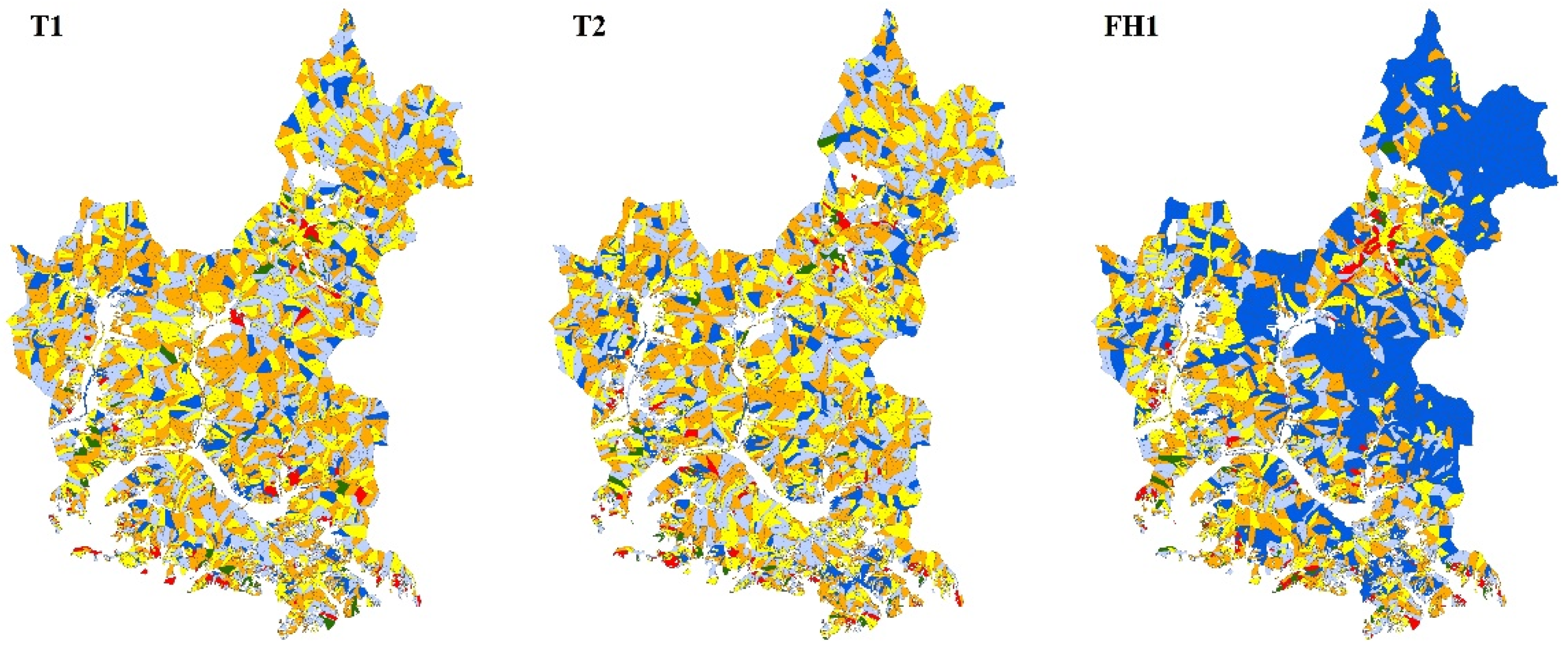
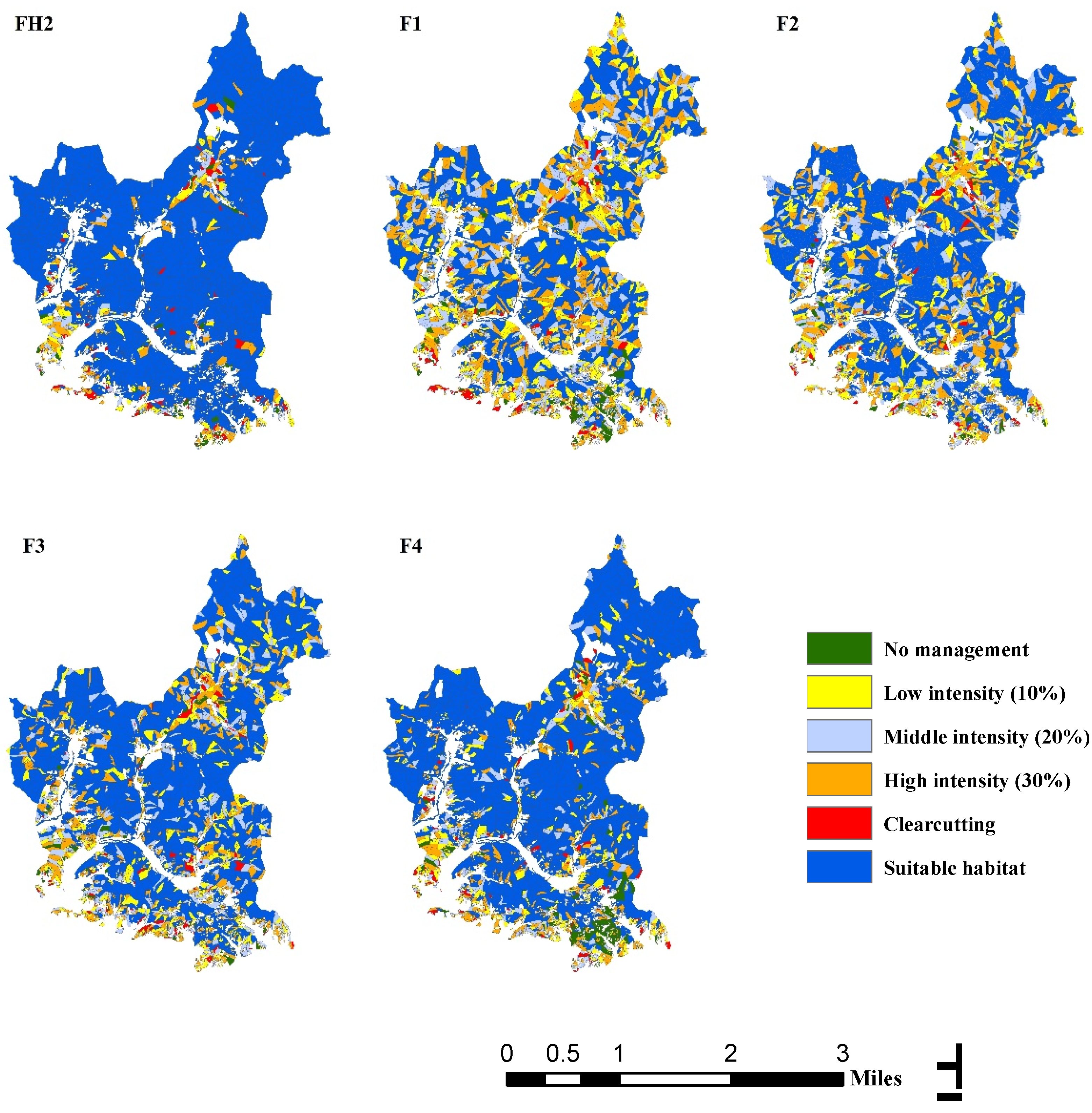
2.6. Management Strategies

To investigate and analyze our planning problems, three management strategies were created for this landscape. The optimization strategies targeted to maximize the forest NPV, solve optimal management combinations, and create the assigned amount of suitable habitat were as follows (Table 2): (1) Timber-oriented management strategy (TMS, scenarios T1 and T2): this model was only constrained by associated timber harvests, i.e., Equation (6) to Equation (11); it should be noted that scenario T1 was assumed as a base scenario for the timber benefits, which did not require spatial harvest restriction and suitable habitat protection. (2) Fixed selection of suitable habitat management strategy (FSSHMS, scenarios FH1 and FH2): in addition to timber harvest constraints, the requirement of conservation of a suitable habitat must be fulfilled; habitat was assigned as suitable if the HSI of the unit exceeded the threshold, i.e., Equation (12) to Equations (13) and (15). (3) Free selection of restricted suitable habitat management strategy (FSRSHMS, scenarios F1 to F4): in addition to timber harvest constraints, the requirement of protection of an assigned amount of suitable habitat must be fulfilled, which could be selected as a suitable habitat if the HSI of the unit exceeded the threshold, i.e., Equation (12) to Equation (15). In this study, we used the minimum gained amount of suitable habitat, calculated as the sum of suitable habitat areas at the beginning of the planning horizon (SHA0) plus the proportions of increase in suitable habitat. The increase in suitable habitat was calculated as the differences between the sum of SHA0 and the sum of potential suitable habitat areas that could be generated with no management throughout the entire planning horizon (PSHAE). In our case, the proportion (i.e., β) was assumed to be 20%, 40%, 60%, and 80%.

2.7. Optimization Algorithm
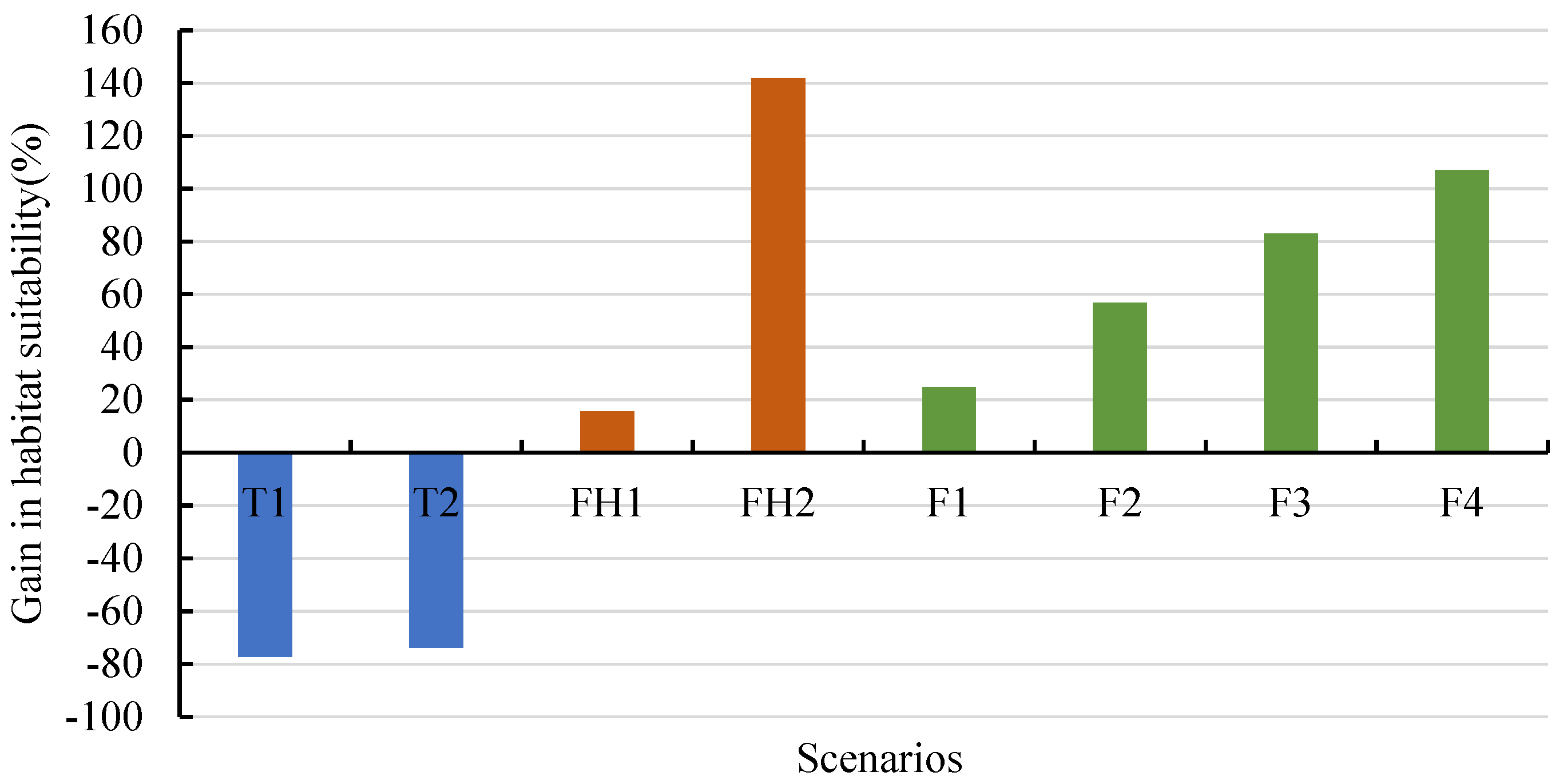
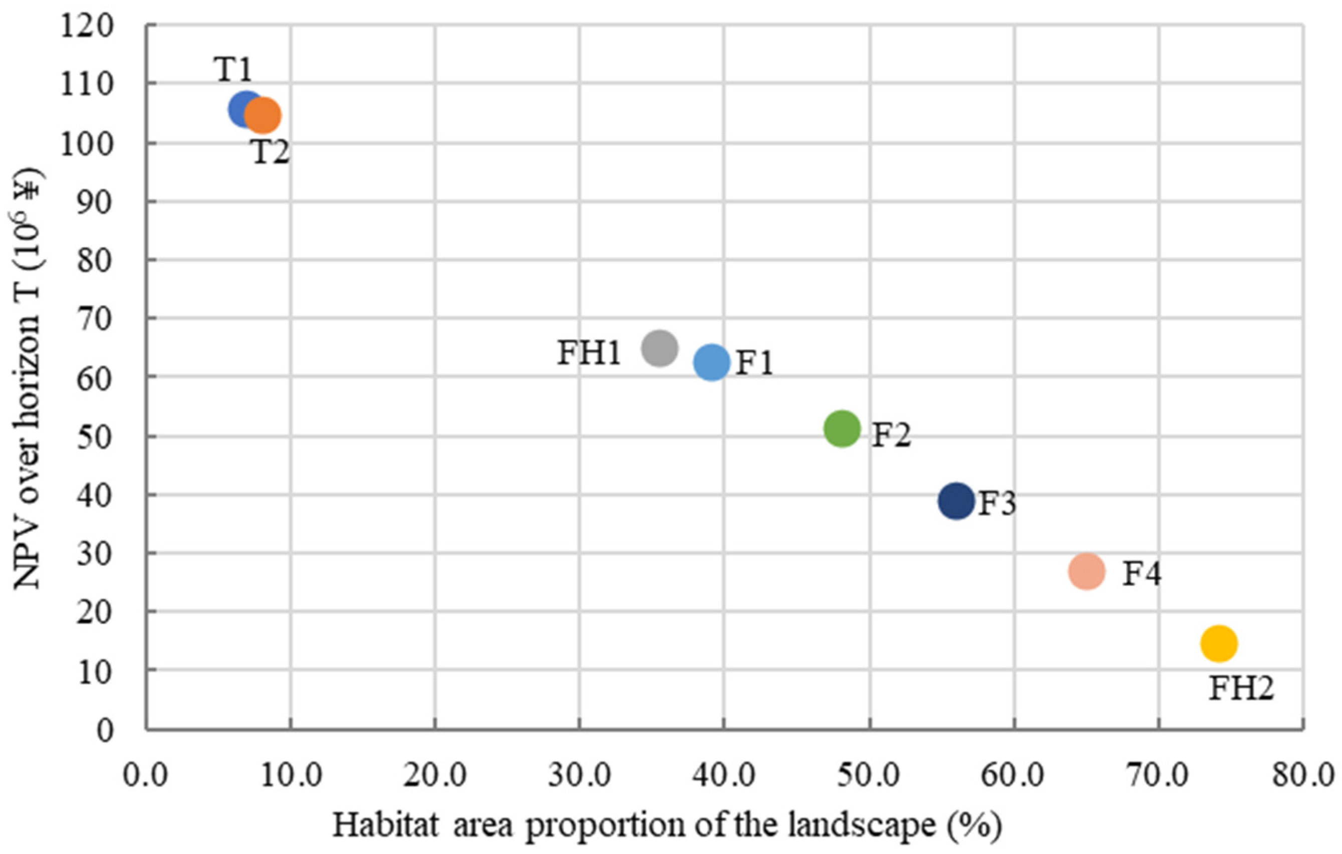
The simulated annealing algorithm was used to solve our planning problems. Simulated annealing has been shown to provide good solutions and avoid local optima [42]. Thus, this algorithm was used to address a set of spatial forest planning problems [23,43]. The principle is to generate a random initial solution at a specified initial temperature, then search for a new solution at random, starting from the neighborhood and selecting that solution based on the optimality of the objective function value. If the solution is an optimized one, it is accepted, and if it is an inferior one, it is accepted or rejected mainly depending on the Metropolis criterion. In this paper, the parameters of the simulated annealing algorithm were set based on a set of trial-and-error tests, i.e., 10,000 degrees for the initial temperature, 1 degree for the termination temperature, 0.999 for the cooling rate, and 300 iterations per temperature. Each simulated scenario was repeated 10 times, and the best solution (i.e., the one with the largest objective function value) would be taken for our analysis to minimize the random effects of the simulated annealing process [23,40]. The planning model was solved to produce each operating scenario using Microsoft Visual Basic 6.0.
p = E x p ( ( f ( x n e w ) f ( x o l d ) ) / T )
where p is the probability of accepting an inferior solution; T is the current temperature; f(xold) is the current objective function value; and f(xnew) is the objective function value of the new solution.
When f(xnew) ≥ f(xold), the current solution is accepted as the new optimal solution (p = 1); when f(xnew) < f(xold), the value of p is influenced by the value of T. The higher the current temperature (T), the higher the probability that an inferior solution would be accepted, while the lower the current temperature (T) and the lower the probability that an inferior solution would be accepted.

3. Results

Timber production over the time period in various planning scenarios is illustrated in Figure 2. In all alternative management strategies, the deviation of timber harvest for each period was relatively stable because of the demand for an even flow of timber harvest in Equation (10). The effect of adjacency constraints was not significant for the timber harvest over the time period between scenarios T1 and T2, and this was mainly because comparatively large openings were assigned in this analysis. Enforcing habitat quality for the great spotted woodpecker notably decreased the timber harvest over the time period, with the average timber harvest losses per period ranging from 30.4% to 75.6%, in comparison with scenario T1.
The distribution of forest areas that were not assigned to any management treatment over the planning horizon by potential age classes is represented in Figure 3. When habitat quality constraints were not enforced, the area of potential relatively old stands (i.e., age class 81–100 and age class > 100) experienced significantly increased harvest levels. When the proportion of suitable habitat in the landscape was between 39% and 65%, the area of potential relatively old stands gradually increased from 42.0% to 57.1%, but the difference in the area of age class 61–80 was minor.
The different benefit–loss levels for the adjacent constraints and the habitat quality maintenance are depicted in Figure 4. The differences between scenario T1 and T2 were moderate (0.9%), primarily owing to the comparatively large openings that were set. As expected, including habitat quality dramatically decreased the total benefit and increased the cost, with NPV losses ranging from 38.4% to 86.0%. When the proportion of suitable habitat in the landscape was between 39% and 65%, the generated NPV loss gradually increased from 40.7% to 74.4%, in comparison with scenario T1. The most marked NPV loss was observed for scenario FH2 (86%), which included PSHAE and was strictly protected over the planning horizon.
The optimal management options of various alternative strategies shown in Figure 5 generated different proportions of maintained habitat quality for the great spotted woodpecker (Figure 6). In TS, the protected habitat proportion significantly decreased, with an average habitat suitability loss of 75.5%. The restriction of habitat quality gradually increased the proportion of suitable habitat in the landscape, with the gain in habitat suitability ranging from 24.7% to 106.9% in FSRSHMS. The differences in habitat suitability gain were small, and the NPV loss was similar between scenarios FH1 and F1 (Figure 4, Figure 6); this was mainly because the fixed selection of suitable habitat in FH1 and the relatively free selection of suitable habitat in F1 generated constraints that differed only slightly but had different spatial assignments (Figure 5).
The trade-offs in dimensions of total timber revenue and the amount of protected habitat are shown in Figure 7. The conflicts were clearly between the timber revenues and the suitable habitat maintenance, with the total NPV decreasing as the suitable habitat amount increased both for designated habitat area limits (FSSHMS) and limits on the amount of suitable habitat area (FSRSHMS) in spatial forest planning problems. Notably, the differences in the obtained value of the suitable habitat amounts throughout the planning horizon between scenario T1 and T2 were not significant, i.e., 7.0% and 8.1% of the landscape, respectively. Similar situations were observed for the relative gain in habitat suitability (Figure 6); scenarios T1 and T2 gained suitable habitat amounts in comparison with SHA0 (73.7% and 77.3%, respectively). This is a result of the other constraints in the planning model, e.g., even flow and minimum average forest age, which limit the total area that can be harvested.

4. Discussion

This study illustrated a spatially explicit forest management planning modeling approach for incorporating habitat quality. We selected the great spotted woodpecker as a goal species and used an HSI model as a tool to learn more about the trade-offs between ecological and economic objectives. The effects related to economic and ecological constraints were quantitatively evaluated for three alternative forest management strategies. We consider this a critical and necessary step for forest managers to examine or select a preferred alternative within biodiversity management in forest planning. However, unlike the results of Mönkkönen et al. [1], in this study, multispecies groups were not included either in habitat quality considerations or economic returns. Finally, similar to other studies [13,44,45], it was revealed that there was a marked total cost in terms of lost timber production and revenue returns when the habitat quality demand increased.
In general, the proportion of old growth stands is the most crucial component in a forest management context [46]. In our case, the old growth stands would be indirectly protected by suitable habitat threshold restrictions. Additionally, the restriction of suitable habitat amount demands would be helpful to retain more old stands, which are a crucial habitat for most species in forest ecosystems. In terms of old growth stands’ conservation, it is similar to the effects of Augustynczik [47], Constantino and Martins [48], which enforced habitat conservation in forest planning problems by restricting mature forests directly.
Spatial restrictions are significant to forests’ ecological and sustainable development [49]. Adjacency constraints have become the most common type of spatial restriction addressed in the spatial forest planning literature. In our TMS, the effects of adjacent constraints were moderate in terms of either total NPV or habitat quality. There are several potential reasons for this result: first, the mean size of management units (approximately 7.82 ± 6.90 ha) across the forest landscape was markedly different from the assumed maximum opening area (40 ha) in this study. Setting different levels of maximum open area is relevant to local forest management policies, solvability of planning problems, and the demands of forest managers. In addition, there were many more potential management prescriptions for each stand in this study than in other studies, and we did not address different parameters of adjacent constraints, e.g., the different green-up periods may have different economic effects [23]. Thus, the limitations of the adjacent constraints were not strict in comparison with other studies [49,50,51]. Nevertheless, on the basis of the various spatial constraints, there is room for many future investigations, such as introducing and exploring the effects of different spatial requirements (e.g., connectivity constraints and core area).
In this study, our hypothesis was that the suitable habitat amount is a crucial factor for the development of species richness and diversity; this is similar to the habitat amount hypothesis proposed by Fahrig [52], i.e., species richness is expected to increase with habitat amount, independently of its spatial configuration within a specific landscape. In addition, the FSSHMS could be considered as a special case of the FSRSHMS in our analysis, whereas the stochastic selection of habitat suitability was not considered in the former, providing a higher degree of flexibility in the planning process. Scenario FH2 implies that forest managers are able and willing to allocate conserved areas at the maximum level to obtain the greatest potential habitat quality. However, as a practical matter, the optimal management option of scenario FH2 is likely to be rarely selected, because it already ignores the benefit demands of forestry organizations. Furthermore, we have not accounted for certain risk factors, e.g., natural and human disturbances, when predicting potential suitable habitat. An opposite approach is depicted in TMS; though TMS provides the optimal solution of the maximum total revenues for forest managers, it is also unlikely to be adopted by forestry organizations in the context of highlighting multi-objective (e.g., ecological, social, and economic goals) forest management.
Scenarios FH1 and F1 to F4 imply different levels of trade-offs between habitat and timber benefits. In the optimal management plans of FSRSHMS, scenarios F2 and F4 would generate NPV losses of 51.5% and 74.4%, respectively. Similar results were shown by Bettinger et al. [44], in which declines in NPV of approximately 24% and 70% were observed when the habitat amount levels were constrained to 40% and 80%, respectively. Additionally, our results reveal that if the minimum suitable habitat target was increased by one percent (approximately 2.28 ha/year), the total NPV would be significantly decreased by an average of approximately 27.31 CNY/ha/yr in FSRSHMS. In fact, there were some error factors in this figure: (1) there were some recovery and maintenance costs that were not taken into account; (2) the economic parameters applied in our analysis were deterministic, such as timber prices, logging costs, and the discount rate; (3) the volume ratios of various species’ timber products were simplified in our analysis, which actually involved different species’ taper equations, site factor, and timber assortment; and (4) some uncertainty factors were not involved in optimal management options, such as stand growth simulations, climate change, and disturbance. Further, by integrating more detail about various timber products’ parameters, and developing adaptive management planning models involving the foregoing quantifiable factors, we can learn more about these compensations.
It is interesting to note that the differences between the total NPV and the timber production of optimal solutions were not significant in FH1 and F1 (Figure 2 and Figure 4), but the spatial assignments of suitable habitats were dramatically different because of the free selection of suitable habitat. The spatial distribution of habitat in FH1 is more clustered than in F1. These clustered habitats may form several connected habitat networks; in the island biogeography theory, suitable habitat connectivity and patch size may have a crucial positive effect on species [53]. In recent studies, Yemshanov et al. [54] have developed a model approach for incorporating the connectivity of habitat protection and timber production in forest management planning. Augustynczik [47] explored the economic effects of imposing habitat connectivity and habitat amount demand in forest planning. Future efforts may be aimed at a more detailed analysis of the trade-offs and conflicts between the habitat networks and harvest benefits along with adjacent constraints of management objectives.
The forest management planning framework in this study can potentially be extended in several ways. Firstly, we focused on a single-species regulatory policy in this planning model. Forest manages also need to consider that different species may prefer different habitat types to the great spotted woodpecker. In such cases, forest managers should consider extending the model to a habitat planning problem for multiple species. Secondly, suitable habitat amounts as a set of constrained variables in this forest planning model is a common approach to incorporating ecological and economic goals in the forest planning model. Essentially, maximizing multiple purposes (e.g., habitat, carbon sequestration, soil, water yield, scenic value, and economic value) leads to hotspot strategies that can guide the sustainable and multifunctional development of forest plans [55], as has been shown by Bagdon et al. [14], Pukkala [56], and Selkimäki et al. [57], who explored a planning model approach to multi-objective forest management planning. Finally, although we assumed thinning was a set of fixed intensities (i.e., 10%, 20%, and 30% of the total volume of a management unit, respectively), in this study, these were reference values for forest management analysis of this region. Future work could be aimed at a more detailed analysis of the trade-offs of different goals, flexible management prescriptions, and spatial harvest requirements.

5. Conclusions

In our study, we formulated an effective model approach to integrated timber revenue and habitat quality in spatial forest management problems. Our results clearly illustrate that suitable habitat amount demand decreased the total benefit markedly. Our optimization planning model provides an efficient approach to learning more about the trade-offs between different objectives that address timber benefits and habitat quality. Furthermore, when biodiversity conservation is addressed in forest management strategies, forest organizations must tailor their habitat selection to local conditions and species demands. The consideration of optimal habitat protection rather than simply greater amounts of habitat could be helpful for balancing and correctly targeting strategies for ecological and economic factors.

Author Contributions

Conceptualization, L.D. and Z.L.; methodology, Y.C. and L.D.; software, Y.C. and L.D.; formal analysis, Y.C.; data curation, Y.C. and L.D.; writing—original draft preparation, Y.C.; writing—review and editing, L.D. and Z.L.; supervision, L.D. and Z.L.; project administration, Z.L.; funding acquisition, Z.L. All authors have read and agreed to the published version of the manuscript.

Funding

This research was funded by the Fundamental Research Funds for the Central Universities of China (Funding number: 2572021DT07).

Data Availability Statement

Not applicable.

Acknowledgments

This work was supported by the Fundamental Research Funds for the Central University.

Conflicts of Interest

The authors declare no conflict of interest.

References

  1. Mönkkönen, M.; Juutinen, A.; Mazziotta, A.; Miettinen, K.; Podkopaev, D.; Reunanen, P.; Salminen, H.; Tikkanen, O.P. Spatially Dynamic Forest Management to Sustain Biodiversity and Economic Returns. J. Environ. Manag. 2014, 134, 80–89. [Google Scholar] [CrossRef] [PubMed]
  2. Price, J.M.; Silbernagel, J.; Nixon, K.; Swearingen, A.; Swaty, R.; Miller, N. Collaborative Scenario Modeling Reveals Potential Advantages of Blending Strategies to Achieve Conservation Goals in a Working Forest Landscape. Landsc. Ecol. 2016, 31, 1093–1115. [Google Scholar] [CrossRef]
  3. von Detten, R.; Hanewinkel, M. Strategies of Handling Risk and Uncertainty in Forest Management in Central Europe. Curr. For. Rep. 2017, 3, 60–73. [Google Scholar] [CrossRef]
  4. Tittler, R.; Messier, C.; Burton, P.J. Hierarchical Forest Management Planning and Sustainable Forest Management in the Boreal Forest. For. Chron. 2001, 77, 998–1005. [Google Scholar] [CrossRef] [Green Version]
  5. Fisher, B.; Edwards, D.P.; Larsen, T.H.; Ansell, F.A.; Hsu, W.W.; Roberts, C.S.; Wilcove, D.S. Cost-Effective Conservation: Calculating Biodiversity and Logging Trade-Offs in Southeast Asia. Conserv. Lett. 2011, 4, 443–450. [Google Scholar] [CrossRef]
  6. Nalle, D.J.; Montgomery, C.A.; Arthur, J.L.; Polasky, S.; Schumaker, N.H. Modeling Joint Production of Wildlife and Timber. J. Environ. Manag. 2004, 48, 997–1017. [Google Scholar] [CrossRef]
  7. Nieuwenhuis, M.; Tiernan, D. The Impact of the Introduction of Sustainable Forest Management Objectives on the Optimisation of PC-Based Forest-Level Harvest Schedules. For. Policy Econ. 2005, 7, 689–701. [Google Scholar] [CrossRef]
  8. Bettinger, P.; Boston, K. Habitat and Commodity Production Trade-Offs in Coastal Oregon. Socioecon. Plann. Sci. 2008, 42, 112–128. [Google Scholar] [CrossRef]
  9. Turner, M.G.; Gardner, R.H. Landscape Ecology in Theory and Practice: Pattern and Process, 2nd ed.; Springer: New York, NY, USA, 2015; p. 237. [Google Scholar]
  10. Edenius, L.; Mikusiński, G. Utility of Habitat Suitability Models as Biodiversity Assessment Tools in Forest Management. Scand. J. For. Res. 2006, 21, 62–72. [Google Scholar] [CrossRef]
  11. Öhman, K.; Edenius, L.; Mikusiński, G. Optimizing Spatial Habitat Suitability and Timber Revenue in Long-Term Forest Planning. Can. J. For. Res. 2011, 41, 543–551. [Google Scholar] [CrossRef] [Green Version]
  12. Pukkala, T.; Sulkava, R.; Jaakkola, L.; Lähde, E. Relationships between Economic Profitability and Habitat Quality of Siberian Jay in Uneven-Aged Norway Spruce Forest. For. Ecol. Manag. 2012, 276, 224–230. [Google Scholar] [CrossRef]
  13. Konoshima, M.; Yoshimoto, A. Balancing Timber Production and Habitat Conservation of Okinawa Rails (Gallirallus Okinawae): Application of a Harvest Scheduling Optimization Model in Subtropical Forest in Okinawa, Japan. J. Mt. Sci. 2019, 16, 2770–2782. [Google Scholar] [CrossRef]
  14. Bagdon, B.A.; Huang, C.-H.; Dewhurst, S. Managing for Ecosystem Services in Northern Arizona Ponderosa Pine Forests Using a Novel Simulation-to-Optimization Methodology. Ecol. Model. 2016, 324, 11–27. [Google Scholar] [CrossRef]
  15. Kline, J.D.; Harmon, M.E.; Spies, T.A.; Morzillo, A.T.; Pabst, R.J.; McComb, B.C.; Schnekenburger, F.; Olsen, K.A.; Csuti, B.; Vogeler, J.C. Evaluating Carbon Storage, Timber Harvest, and Habitat Possibilities for a Western Cascades (USA) Forest Landscape. Ecol. Appl. 2016, 26, 2044–2059. [Google Scholar] [CrossRef]
  16. Mazziotta, A.; Podkopaev, D.; Triviño, M.; Miettinen, K.; Pohjanmies, T.; Mönkkönen, M. Quantifying and Resolving Conservation Conflicts in Forest Landscapes via Multiobjective Optimization. Silva Fenn. 2017, 51, 1778. [Google Scholar] [CrossRef]
  17. Dupont, S.; Ikonen, V.-P.; Väisänen, H.; Peltola, H. Predicting Tree Damage in Fragmented Landscapes Using a Wind Risk Model Coupled with an Airflow Model. Can. J. For. Res. 2015, 45, 1065–1076. [Google Scholar] [CrossRef]
  18. Baskent, E.Z.; Keles, S. Spatial Forest Planning: A Review. Ecol. Model. 2005, 188, 145–173. [Google Scholar] [CrossRef]
  19. Stang, M.B.; Arce, J.E.; do Amaral Machado, S.; Belavenutti, P.H.; Fiorentin, L.D. Spatial Forest Planning for Optimized Harvest Scheduling. Floresta E Ambiente 2019, 26, e20160100. [Google Scholar] [CrossRef]
  20. Murray, A.T. Spatial Restrictions in Harvest Scheduling. For. Sci. 1999, 45, 45–52. [Google Scholar]
  21. McDill, M.E.; Rebain, S.A.; Braze, J. Harvest Scheduling with Area-Based Adjacency Constraints. For. Sci. 2002, 48, 631–642. [Google Scholar] [CrossRef]
  22. Irene, D.P.L.; Hoganson, H.M.; Carson, M.T.; Windmuller-Campione, M. Recognizing Spatial Considerations in Forest Management Planning. Curr. For. Rep. 2017, 3, 308–316. [Google Scholar] [CrossRef]
  23. Dong, L.; Lu, W.; Liu, Z. Developing Alternative Forest Spatial Management Plans When Carbon and Timber Values Are Considered: A Real Case from Northeastern China. Ecol. Model. 2018, 385, 45–57. [Google Scholar] [CrossRef]
  24. Cyr, G.; Raulier, F.; Fortin, D.; Pothier, D. Using Operating Area Size and Adjacency Constraints to Mitigate the Effects of Harvesting Activities on Boreal Caribou Habitat. Landsc. Ecol. 2017, 32, 377–395. [Google Scholar] [CrossRef]
  25. Wang, H.Z. Dynamic Simulating System for Stand Growth of Forests in Northeast China. Ph.D. Thesis, Northeast Forestry University, Harbin, China, 2012. (In Chinese). [Google Scholar]
  26. Dong, L.; Lu, W.; Liu, Z. Determining the Optimal Rotations of Larch Plantations When Multiple Carbon Pools and Wood Products Are Valued. For. Ecol. Manag. 2020, 474, 118356. [Google Scholar] [CrossRef]
  27. Drever, M.C.; Aitken, K.E.H.; Norris, A.R.; Martin, K. Woodpeckers as Reliable Indicators of Bird Richness, Forest Health and Harvest. Biol. Conserv. 2008, 141, 624–634. [Google Scholar] [CrossRef]
  28. Roberge, J.-M.; Angelstam, P.; Villard, M.-A. Specialised Woodpeckers and Naturalness in Hemiboreal Forests—Deriving Quantitative Targets for Conservation Planning. Biol. Conserv. 2008, 141, 997–1012. [Google Scholar] [CrossRef]
  29. Blanc, L.A.; Martin, K. Identifying Suitable Woodpecker Nest Trees Using Decay Selection Profiles in Trembling Aspen (Populus Tremuloides). For. Ecol. Manag. 2012, 286, 192–202. [Google Scholar] [CrossRef]
  30. van der Hoek, Y.; Gaona, G.V.; Martin, K. The Diversity, Distribution and Conservation Status of the Tree-Cavity-Nesting Birds of the World. Divers. Distrib. 2017, 23, 1120–1131. [Google Scholar] [CrossRef] [Green Version]
  31. Heilongjiang Forestry and Grassland Administration. List of Provincial Key Protected Wild Animals. Harbin: Heilongjiang Forestry and Grassland Administration. Available online: https://www.doc88.com/p-605951168974.html?s=rel&id=1 (accessed on 29 November 2021).
  32. Barrientos, R. Retention of Native Vegetation within the Plantation Matrix Improves Its Conservation Value for a Generalist Woodpecker. For. Ecol. Manag. 2010, 260, 595–602. [Google Scholar] [CrossRef]
  33. Yang, Y. Study on Habitat Selection and Habitat Assessment of Picoides major. Master’s Thesis, Beijing Forestry University, Beijing, China, 2011. (In Chinese). [Google Scholar]
  34. Zhao, Z. Fauna of Rare and Endangered Species of Vertebrates of Northeast China; China Forestry Publishing House: Beijing, China, 1999; pp. 428–430. (In Chinese) [Google Scholar]
  35. Pasinelli, G. Nest Site Selection in Middle and Great Spotted Woodpeckers Dendrocopos Medius & D. Major: Implications for Forest Management and Conservation. Biodivers. Conserv. 2007, 16, 1283–1298. [Google Scholar] [CrossRef] [Green Version]
  36. Hebda, G. Nesting Sites of the Great Spotted Woodpecker Dendrocopos Major L. in Poland: Analysis of Nest Cards. Pol. J. Ecol. 2009, 57, 149–158. [Google Scholar]
  37. Rolstad, J.; Rolstad, E.; Stokke, P.K. Feeding Habitat and Nest-Site Selection of Breeding Great Spotted Woodpeckers Dendrocopos Major. Ornis Fenn. 1995, 72, 62–71. [Google Scholar]
  38. Deng, W.-H.; Gao, W. Edge Effects on Nesting Success of Cavity-Nesting Birds in Fragmented Forests. Biol. Conserv. 2005, 126, 363–370. [Google Scholar] [CrossRef]
  39. Wiacek, J.; Polak, M.; Kucharczyk, M.; Bohatkiewicz, J. The Influence of Road Traffic on Birds during Autumn Period: Implications for Planning and Management of Road Network. Landsc. Urban Plan. 2015, 134, 76–82. [Google Scholar] [CrossRef]
  40. Dong, L.; Bettinger, P.; Liu, Z.; Qin, H. A Comparison of a Neighborhood Search Technique for Forest Spatial Harvest Scheduling Problems: A Case Study of the Simulated Annealing Algorithm. For. Ecol. Manag. 2015, 356, 124–135. [Google Scholar] [CrossRef]
  41. DB23/T 870-2004; Merchantable Volume Ratio Tables of Main Tree Species in Heilongjiang Province. Heilongjiang Forestry and Grassland Administration: Harbin, China. Available online: https://max.book118.com/html/2016/0101/32487748.shtm (accessed on 5 November 2021). (In Chinese)
  42. Jin, X.; Pukkala, T.; Li, F. Fine-Tuning Heuristic Methods for Combinatorial Optimization in Forest Planning. Eur. J. For. Res. 2016, 135, 765–779. [Google Scholar] [CrossRef]
  43. Lockwood, C.; Moore, T. Harvest Scheduling with Spatial Constraints: A Simulated Annealing Approach. Can. J. For. Res. 1993, 23, 468–478. [Google Scholar] [CrossRef]
  44. Bettinger, P.; Johnson, D.L.; Johnson, K.N. Spatial Forest Plan Development with Ecological and Economic Goals. Ecol. Model. 2003, 169, 215–236. [Google Scholar] [CrossRef]
  45. Kašpar, J.; Róbert, R.; Hlavatý, R. A Forest Planning Approach with Respect to the Creation of Overmature Reserved Areas in Managed Forests. Forests 2015, 6, 328–343. [Google Scholar] [CrossRef] [Green Version]
  46. Laginha Pinto Correia, D.; Raulier, F.; Filotas, É.; Bouchard, M. Stand Height and Cover Type Complement Forest Age Structure as a Biodiversity Indicator in Boreal and Northern Temperate Forest Management. Ecol. Indic. 2017, 72, 288–296. [Google Scholar] [CrossRef]
  47. Augustynczik, A.L.D. Habitat Amount and Connectivity in Forest Planning Models: Consequences for Profitability and Compensation Schemes. J. Environ. Manag. 2021, 283, 111982. [Google Scholar] [CrossRef] [PubMed]
  48. Constantino, M.; Martins, I. Branch-and-Cut for the Forest Harvest Scheduling Subject to Clearcut and Core Area Constraints. Eur. J. Oper. Res. 2018, 265, 723–734. [Google Scholar] [CrossRef]
  49. Yoshimoto, A.; Asante, P. Focal-Point Aggregation Under Area Restrictions through Spatially Constrained Optimal Harvest Scheduling. For. Sci. 2019, 65, 164–177. [Google Scholar] [CrossRef]
  50. Boston, K.; Bettinger, P. An Economic and Landscape Evaluation of the Green-up Rules for California, Oregon, and Washington (USA). For. Policy Econ. 2006, 8, 251–266. [Google Scholar] [CrossRef]
  51. Toth, S.F.; McDill, M.E.; Koennyue, N.; George, S. Testing the Use of Lazy Constraints in Solving Area-Based Adjacency Formulations of Harvest Scheduling Models. For. Sci. 2013, 59, 157–176. [Google Scholar] [CrossRef]
  52. Fahrig, L. Rethinking Patch Size and Isolation Effects: The Habitat Amount Hypothesis. J. Biogeogr. 2013, 40, 1649–1663. [Google Scholar] [CrossRef]
  53. Bueno, A.S.; Peres, C.A. Patch-Scale Biodiversity Retention in Fragmented Landscapes: Reconciling the Habitat Amount Hypothesis with the Island Biogeography Theory. J. Biogeogr. 2019, 46, 621–632. [Google Scholar] [CrossRef] [Green Version]
  54. Yemshanov, D.; Haight, R.G.; Liu, N.; Rempel, R.S.; Koch, F.H.; Rodgers, A. Balancing Large-Scale Wildlife Protection and Forest Management Goals with a Game-Theoretic Approach. Forests 2021, 12, 809. [Google Scholar] [CrossRef]
  55. Baskent, E.Z. A Framework for Characterizing and Regulating Ecosystem Services in a Management Planning Context. Forests 2020, 11, 102. [Google Scholar] [CrossRef] [Green Version]
  56. Pukkala, T. Which Type of Forest Management Provides Most Ecosystem Services? For. Ecosyst. 2016, 3, 9. [Google Scholar] [CrossRef] [Green Version]
  57. Selkimäki, M.; González-Olabarria, J.R.; Trasobares, A.; Pukkala, T. Trade-Offs between Economic Profitability, Erosion Risk Mitigation and Biodiversity in the Management of Uneven-Aged Abies Alba Mill. Stands. Ann. For. Sci. 2020, 77, 12. [Google Scholar] [CrossRef] [Green Version]
Figure 1. Initial distribution of forest areas by different forest types and age classes.
Forests 13 00525 g001
Figure 2. Timber production of Maoershan Forest Farm, China, over the time period of alternative management strategies: timber-oriented management strategy (TMS, scenarios T1 and T2), fixed selection of suitable habitat management strategy (FSSHMS, scenarios FH1 and FH2), and free selection of restricted suitable habitat management strategy (FSRSHMS, scenarios F1 to F4).
Forests 13 00525 g002
Figure 3. Distribution of forest areas that were not assigned to any management treatment by potential age classes (years) at Maoershan Forest Farm, China, over a 50-year planning horizon of alternative management strategies: timber-oriented management strategy (TMS, scenarios T1 and T2), fixed selection of suitable habitat management strategy (FSSHMS, scenarios FH1 and FH2), and free selection of restricted suitable habitat management strategy (FSRSHMS, scenarios F1 to F4).
Forests 13 00525 g003
Figure 4. Net present value (NPV) loss proportion of timber production incurred in alternative management strategies for Maoershan Forest Farm, China, compared to scenario T1. The bars represent scenarios within the strategies: timber-oriented management strategy (TMS, scenario T2), fixed selection of suitable habitat management strategy (FSSHMS, scenarios FH1 and FH2), and free selection of restricted suitable habitat management strategy (FSRSHMS, scenarios F1 to F4).
Forests 13 00525 g004
Figure 5. The spatial assignment of optimal management prescriptions of various alternative strategies for timber production at Maoershan Forest Farm, China: timber-oriented management strategy (TMS, scenarios T1 and T2), fixed selection of suitable habitat management strategy (FSSHMS, scenarios FH1 and FH2), and free selection of restricted suitable habitat management strategy (FSRSHMS, scenarios F1 to F4).
Forests 13 00525 g005aForests 13 00525 g005b
Figure 6. Relative gain (%) in habitat suitability for the great spotted woodpecker (Dendrocopos major) at Maoershan Forest Farm, China, compared to the suitable habitat area at beginning of planning horizon with alternative management strategies: timber-oriented management strategy (TMS, scenarios T1 and T2), fixed selection of suitable habitat management strategy (FSSHMS, scenarios FH1 and FH2), and free selection of restricted suitable habitat management strategy (FSRSHMS, scenarios F1 to F4).
Forests 13 00525 g006
Figure 7. Trade-offs between the optimal solutions for various management strategies in dimensions of total timber revenue and the amount of protected suitable habitat for the great spotted woodpecker (Dendrocopos major) in the landscape of Maoershan Forest Farm, China. NPV: net present value. Colored circles represent scenarios within the strategies: timber-oriented management strategy (TMS, scenarios T1 and T2), fixed selection of suitable habitat management strategy (FSSHMS, scenarios FH1 and FH2), and free selection of restricted suitable habitat management strategy (FSRSHMS, scenarios F1 to F4).
Forests 13 00525 g007
Table 1. Overview of the management treatments for the planning problem.
Management TreatmentAge Limit for Forest Types 4 (Year)Description
No managementNBF, NPF, LP, and MP: <21;
NOF and NMBF: <41
Any management treatments when stand age is younger than the limiting ages are strictly prohibited.
Low intensity 1NBF and NPF: ≥21;
LP and MP: ≥21 and <41;
NOF and NMBF: ≥41
Can only be assigned to one of the three intensities of thinning, or no management, when stand age falls within the interval of the limiting ages.
Middle intensity 2
High intensity 3
ClearcuttingLP and MP: ≥41Only LP and MP can be assigned to clearcutting when stand age exceeds the limiting ages, and they can be assigned to thinning or no management, too.
1 Low intensity: 10% of the total volume of a unit. 2 Middle intensity: 20% of the total volume of a unit. 3 High intensity: 30% of the total volume of a unit. 4 Age limit for forest types: involves six forest types., i.e., NBF: natural birch forests, NPF: natural poplar forests, NOF: natural oak forests, NMBF: natural mixed-broadleaf forests, LP: larch plantation, and MP: Mongolian pine plantation.
Table 2. Overview of the various management scenarios for the planning problem.
Management
Scenarios
ObjectiveAdjacent
Constraints
Habitat Quality
Constraints
Planning
Formulations
T1Maximize NPV2 periods of green-up
constraint;
Umax = 40 ha.
Equations (6)–(10)
T2 Equations (6)–(11)
FH1HSIitHSIsuit;
t = 0.
Equations (6)–(13) and (15)
FH2HSIitHSIsuit;
t = 0, 1, 2, 3, …, 10.
Equations (6)–(13) and (15)
F1HSIitHSIsuit;
β = 0.39 1;
t = 0, 1, 2, 3, …, 10.
Equations (6)–(15)
F2HSIitHSIsuit;
β = 0.48 2;
t = 0, 1, 2, 3, …, 10.
Equations (6)–(15)
F3HSIitHSIsuit;
β = 0.56 3;
t = 0, 1, 2, 3, …, 10.
Equations (6)–(15)
F4HSIitHSIsuit;
β = 0.65 4;
t = 0, 1, 2, 3, …, 10.
Equations (6)–(15)
1 β = 0.39: The level in SHA0 + 20% of the difference between the sum of SHA0 and PSHAE. 2 β = 0.48: The level in SHA0 + 40% of the difference between the sum of SHA0 and PSHAE. 3 β = 0.56: The level in SHA0 + 60% of the difference between the sum of SHA0 and PSHAE. 4 β = 0.65: The level in SHA0 + 80% of the difference between the sum of SHA0 and PSHAE.
Publisher’s Note: MDPI stays neutral with regard to jurisdictional claims in published maps and institutional affiliations.

