Article

Habitat Suitability Modeling of Rare Turkeybeard (Xerophyllum asphodeloides) Species in the Talladega National Forest, Alabama, USA

1
Warnell School of Forestry and Natural Resources, University of Georgia, 180 E. Green Street, Athens, GA 30602, USA
2
US Forest Service, Talladega National Forest, 45 Highway 281, Heflin, AL 36264, USA
*
Author to whom correspondence should be addressed.
Forests 2022, 13(4), 490; https://doi.org/10.3390/f13040490
Submission received: 3 February 2022 / Revised: 14 March 2022 / Accepted: 15 March 2022 / Published: 22 March 2022
(This article belongs to the Section Forest Inventory, Modeling and Remote Sensing)

Abstract

:
This study focused on the rare and threatened plant species eastern turkeybeard (Xerophyllum asphodeloides (L.) Nutt.) and its presence or absence in the Talladega National Forest in Alabama, USA. An ensemble suitable habitat map was developed using four different modeling methods (MaxEnt, Generalized Linear Model, Generalized Additive Model, and Random Forest). AUC evaluation scores for each model were 0.99, 0.96, 0.98, and 0.99, respectively. Biserial correlation scores for models ranged from 0.71 (GLM) to 0.94 (RF). The four different models agreed suitable habitat was found to cover 159.57 ha of the land. The ground slope variable was the most contributive variable in the MaxEnt and RF models and was also significant in the GLM and GAM models. The knowledge gained from this research can be used to establish and implement habitat suitability strategies across the Talladega National Forest and similar ecosystems in the southern United States.

1. Introduction

Turkeybeard (Xerophyllum asphodeloides (L.) Nutt.) is a perennial understory forest herb that grows in discreet mountain populations in the eastern United States, from Virginia to Alabama. The plant occurs naturally in forested areas of these states as well in the Pine Barrens of Southern New Jersey and thus is found in 10 states [1,2,3,4]. Turkeybeard is native to North America and is classified as a rare and threatened species in some states and at the national level [5,6,7]. There is only one published study [3] that offered a predictive habitat suitability model for turkeybeard, which was situated in western and eastern Virginia. Bourg et al. [3] described a set of environmental variables that might correlate well with turkeybeard occurrences: elevation, slope, forest type, and fire frequency.
To manage natural areas in a sustainable manner, habitat modeling approaches are necessary for evaluating current and desired future conditions of forests. It has been suggested that ideal management plans for public forest lands would have a conservation perspective, provide a set of sustainable goals, and employ habitat modeling approaches [8,9]. For instance, forest management goals might state a need to increase plant species diversity and restore the natural integrity of a forested landscape. Therefore, a critical aspect of forest management is to use habitat models to gauge the development direction of a forest when management activities are employed [10]. Managing forest areas using sustainable approaches has become a worldwide issue [11]. Over the past 30 years, scientists and experts have used habitat modeling approaches to make informed decisions concerning the management of forestlands for biodiversity conservation [8,10]. In fact, the U.S. national forests are currently managed under an approach that focuses on the sustainability of ecosystems [12]. In this regard, habitat suitability models may be of value in assessing current and future trajectories of certain forest conditions.
Giles [13] defines a Habitat Suitability Index (HSI) as an index of the carrying capacity of an area for a given species. The United States Fish and Wildlife Service [14] quantified habitat suitability as an organism’s life requisites, using the structure, composition, and spatial components of habitat. Habitat models, therefore, allow quantification of habitat suitability as a proxy for the response of a species to an environment [15]. The development of habitat suitability indices has been driven by advances in data processing capacity and analysis techniques, shifts in scientific paradigms, and increased attention to environmental heterogeneity and scale issues [16].
Since habitat-related information is often derived from forest inventories, one can potentially produce habitat suitability models that are a function of forest character and forest management history. With the many, easy to implement, modeling approaches available today, it thus becomes critical to address several conceptual and methodological issues when constructing these models [10]. A habitat suitability modeling process ideally follows five steps: conceptualization, data preparation, model calibration (fitting), model evaluation, and spatial prediction [17]. With respect to model fitting and spatial prediction, several analytical methods have recently been employed for developing habitat suitability models, including generalized linear models (GLM) [18], classification and regression trees (CART) [19], random forest (RF) [20], artificial neural networks (ANN) [21], generalized additive models (GAM) [22], and maximum entropy (MaxEnt) approaches [23].
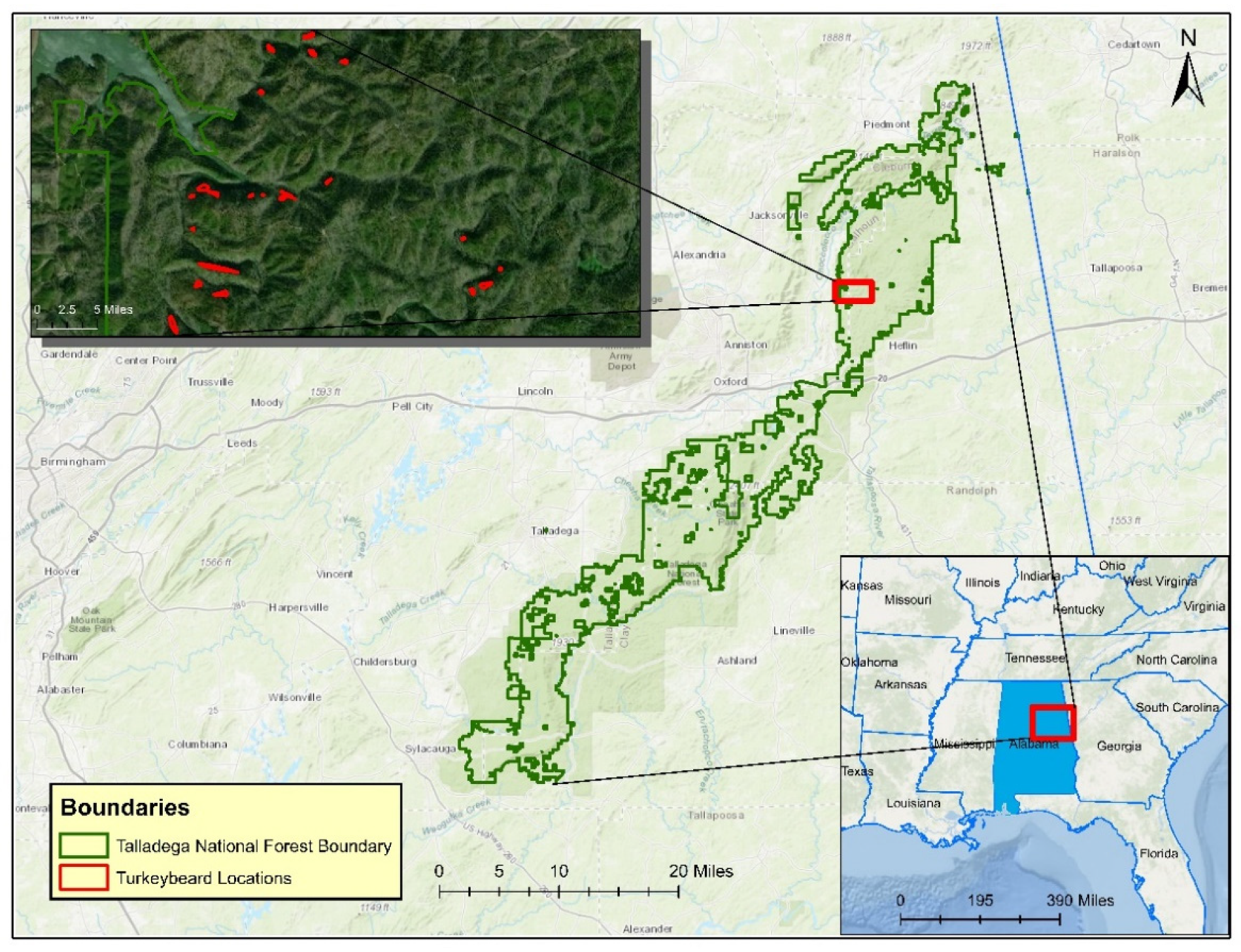
In this paper, we use this prior work [3] to inform a new ensemble model to predict relative habitat suitability across the Talladega National Forest (TNF). This represents the first effort to model a potentially suitable habitat for the rare turkeybeard in the southern part of its range. We discuss how this model can be used to inform forest management, and also address some limitations associated with modeling rare species. We hypothesize that through the development of a habitat model, the highest valued habitat can be identified by a consistent prediction of it through four different models, and the correlation between the presence of the plant and the highly valued habitat is positive and relatively good.

2. Materials and Methods

2.1. Study Area

The TNF is located in northeastern Alabama, USA. It was mainly purchased as forest reserves from private landowners in the early 1900s through provisions contained in the Weeks Law of 1911 (P.L. 61-435, Chapter 186) to help regulate the flow of navigable streams in the headwaters of watersheds located mainly in the eastern United States. Since its proclamation as a national forest in 1936, the TNF has been managed by the US Forest Service [24]. The forest is physically separated into two areas, and these are further allocated into three Ranger Districts: Oakmulgee Ranger District, Shoal Creek Ranger District, and Talladega Ranger District. In all, the national forest is located in 11 Alabama counties. However, the study area involves the Shoal Creek and Talladega Ranger Districts, which are located in Calhoun, Clay, Cleburne, Cherokee, and Talladega counties. The lands of the TNF are situated in the Talladega Mountains, a part of the Piedmont, and Ridge and Valley ecoregions of the United States [25] (Figure 1).
The climate of the TNF is considered humid subtropical, with hot and humid summers and mild winters. In this area, the annual precipitation is about 1260 mm, the annual maximum temperature is about 23.83 °C, and the annual minimum temperature is about 10.16 °C [26]. The TNF is composed of 95,276 ha of land and there are three main vegetation types: mixed coniferous and deciduous forests, deciduous forests, and coniferous forests. These vegetation types generally include broadleaf hardwood (deciduous), natural pine, and planted pine forests. Nearly 52% of the TNF is composed of forests dominated by four coniferous tree species: loblolly pine (Pinus taeda L.), longleaf pine (Pinus palustris Mill.), shortleaf pine (Pinus echinata Mill.), and Virginia pine (Pinus virginiana Mill.) [27].

2.2. Occurrence Data

X. asphodeloides [1,2] is a rare and threatened plant species native to the United States and is mainly located in 10 eastern states [5,6,7]. To our knowledge, there seems to be no complete database containing the plant’s occupancy on the TNF other than site visit records from the TNF. We obtained 22 occurrence locations of the species, consisting of polygons that represent turkeybeard patches (Figure 1). The number of individual plants in these sites ranged from 28 to 1618, but individual plant locations were not available. These plant population areas comprise a total of only 2.62 hectares across the study area. Occurrence polygons ranged between 18.94 and 5022.23 square meters in size. Patches of turkeybeard were identified and delineated by TNF staff between 2015 and 2021.
In addition, we traveled to the TNF to collect occurrence data through new field surveys and to validate the already-identified occurrence locations. Each patch location was noted using a Trimble Juno T41 GNSS (Global Navigation Satellite System) receiver which has a horizontal accuracy of about 2 m in forested conditions [28]. An ad-hoc survey was conducted for 7 h on 1 day. With the assistance of a US Forest Service employee, we visited six sites to determine the presence of turkeybeard. Three of these sites were already known turkeybeard population locations, and we confirmed its presence. We confirmed the three known occurrence locations using Google Earth Pro, and we verified that the locations where we collected points matched occurrence points collected by TNF staff. Three other sites were identified using a preliminary analysis conducted by another researcher; however, we were not able to find new occurrence data at those sites. Due to COVID restrictions placed on access to the TNF by the U.S. government, we were unable to search for further locations of the plant. Therefore, in this work, we used 22 presence-only locations of turkeybeard from the national forest’s observations. Using ArcMap 10.8, we generated point data for each location occurrence polygon representing the centroid of each of the 22 presence-only locations.

2.3. Environmental Variables

In this study, biotic and abiotic variables were used to develop a relationship with turkeybeard occurrences. Twenty-eight abiotic and biotic variables were selected for this analysis: 3 were geomorphic (elevation, aspect, and ground slope), 6 were soil-related (water content, soil organic material, soil percentage of clay, soil percentage of sand, soil percentage of silt, and soil PH), and 19 were bioclimate variables. The geographic information system (GIS) databases of 19 bioclimate variables were obtained from the WorldClim (WorldClim version 2.1) website ([29], https://www.worldclim.org/data/worldclim21.html, accessed on 16 January 2022). A detailed explanation of these variables can be found in Appendix A. A 30 m digital elevation model (DEM) was obtained from the United States Department of Agriculture (USDA) Natural Resources Conservation Service Geospatial Data Gateway ([30], https://datagateway.nrcs.usda.gov/GDGOrder.aspx, accessed on 16 January 2022), and this was used to calculate aspect and slope using the surface analysis tools in ArcGIS. Soil data were obtained from the USDA SSURGO (Soil Survey Geographic Database) database [31]. All data were resampled to a 30 m spatial resolution (if not already available at that resolution) using the nearest neighbor technique. These variables were also projected to NAD 1983 UTM Zone 16N. The TNF property boundary was used as an extent for all variables for analyses.

2.4. Habitat Suitability Modeling

We used four common algorithms to model suitable habitats for turkeybeard; GLM, GAM, MaxEnt, and Random Forests (RF). All four modeling efforts were conducted using R 3.5.2 software. The resulting map predictions were then exported to ArcMap and a final ensemble model was produced using map algebra.

2.4.1. Variable Preparation and Selection

To reduce multicollinearity, one of two strongly correlated variables was removed from the analysis by evaluating the correlation coefficient and the variance inflation factor (VIF). The Pearson Correlation Coefficient (Pearson’s r) is a linear correlation coefficient that returns a value between −1 and +1 with values closer to +1 indicating a positive correlation, values closer to −1 indicating a negative correlation, and a value of 0 indicating no correlation between variables. Based on the literature, there is no certain rate of the threshold for a decision to remove one variable from the analysis. However, removing variables above the threshold of r = 0.8 is recommended by Menard [32] and r = 0.7 is recommended by Green [33]. Further, after a correlation assessment, there may still be a missing correlated structure that cannot be seen in pairwise correlations [17]. To address these issues, the VIF test recommended by Harrell [34], Guisan et al. [35], Hair et al. [36], and Guisan et al. [17] was used. A VIF value below 10.0 suggested the model did not have a collinearity problem [17,37], and a correlation below r = 0.7 suggested no strong correlation among the two variables. Once the highly correlated variables were removed from the analysis, each of the different modeling methods (described below) was applied separately.

2.4.2. Generalized Linear Model

GLMs are statistical extensions of linear models that do not impose unnatural scales of data and thus allow for structures of non-linearity and non-constant variation in the data. GLM is a generalization of multiple regression analysis that uses a binomial distribution and a logistic relation to suit polynomials of higher degrees of complexity greater than linear [38]. In GLMs the mean of the response is determined by the linear predictor [18]. They are based on an implied relationship between the mean of the response variable and the explanatory variable’s linear combination [22,39]. For the GLM analysis, 1000 random pseudo-absences were generated, 90% of these points were used as training points and 10% were used for validation testing. A high number of pseudo-absences relative to presence locations was used to reflect the high amount of vegetative variability across the landscape. For the model selection and generation, stepAIC stepwise regression analysis function from the MASS library in R was used to select the best model based on their Akaike information criterion (AIC) score, and the best model was selected. This best model was run 10 times and the solution with the lowest AIC score (the best) was the model selected.

2.4.3. Generalized Additive Model

Instead of being algorithm-driven, GAMs are data-driven; that is, the resulting fitted values do not originate from an a priori model [40]. GAMs employ “smoother” algorithms, which automatically match response curves “as closely as possible” to the data provided the degree of smoothing allowed [17]. GAMs are semi-parametric extensions of GLMs [39]. Thus, instead of being constrained by the shapes available in a parametric class, GAMs allow the data to decide the form of the response curves [22,39,40]. For the GAM analysis, 1000 random pseudo-absences were generated, and 90% were used as training points while 10% were used for validation testing. For model selection and generation, step.Gam function from the gam library in R was used, a stepwise regression analysis was used to model selection based on AIC scores. In a GAMs model, an ANOVA test is also applied to select the best solution. This model was run 10 times (like the GLM) and the solution that had the lowest AIC score (the best model) was selected.

2.4.4. MaxEnt

MaxEnt estimates a target probability distribution by finding the probability distribution of maximum entropy, which is subject to a series of restrictions that represent our imperfect knowledge about the target distribution [23]. MaxEnt calculates the likelihood that the environment will be suitable by estimating the distribution of maximum entropy based on both occurrence records and a set of randomly generated background (pseudo-absence) points. GLMs, GAMs, and machine learning techniques such as MaxEnt have clear parallels with some existing methods for predicting species distributions [23]. Although MaxEnt is similar to GLMs and GAMs, GLMs and GAMs are discriminative methods, and they require both occurrence and absence data. However, MaxEnt is a generative method: it can operate without absence data [23] and it may also be effective with a small amount of training data [23,41,42,43]. For the MaxEnt analysis, 1000 random background points were generated. Of these, 90% were used as training points and 10% were used for validation testing. MaxEnt was run 10 times like the GLM and GAM methods. However, unlike the GLM and GAM models, after the 10 runs, the MaxEnt results were averaged to produce the final prediction.

2.4.5. Random Forest

RF is a form of machine learning algorithm which provides a metric of variable significance, both for classification and for regression [44], and it executes a combination of tree predictors [20]. The RF is a non-parametric tree-based approach that involves a large number of classification and regression trees that are expanded regression tree models. RF prevents over-fitting by using stochasticity in the tree-building process as well as at each node [20]. Three parameters must be taken into account when creating an RF: the proportion of sub-samples, the number of optimal estimators in each node, and the optimal number of trees [45]. For the RF analysis, 1000 random background points (pseudo-absences) were generated, and 90% were used as training points, while 10% were used for validation testing. RF was run 10 times like the other methods. Like the MaxEnt model, the outcomes from 10 runs were averaged and used for prediction and generating a suitability map.
RF has been shown to be sensitive to a class imbalance (low number of presence points vs. high number of pseudo-absence points), and it has been suggested that down-sampling (using the same number of presence and pseudo-absence points) or weighting might improve its performance [46]. However, it has also been suggested that when models such as these are applied, the pseudo-absence points should adequately represent the variation in environmental covariates and all types of environments in the area of interest should be represented [46]. Given the highly diverse nature of the forests within the large area of the TNF, and the low number (22) of known presences of turkeybeard, we made a difficult decision to use the same assumptions with RF as were used with the other models, knowing that the proportion of background (pseudo-absence) points may lead to biases in the results.

2.4.6. Final Habitat Suitability

Final suitability prediction maps from each of the four models (MaxEnt, GLM, GAM, RF) were reclassified as 0 (Unsuitable) and 1 (Suitable) and their thresholds were calculated based on the evaluation for each model with the use of the sensitivity-specificity sum maximization approach recommended by Liu et al. [47]. In this approach, the suitability value at which the sum of the sensitivity (true positive rate) and specificity (true negative rate) is highest is chosen as a threshold to reclassify the continuous predictions into suitable/unsuitable. After this reclassification step, all predictions were summed, creating five different classes with values 0, 1, 2, 3, 4. These classes represent suitable habitat locations not predicted by any of the four models (0), places predicted by only one model (1), places predicted by two models in which both overlapped or agreed (2), places predicted by three models in which all three overlapped or agreed (3), and places predicted by all four models in which all four overlapped or agreed (4). The fourth class represents the most highly suitable areas and the value of 0 represents the most unsuitable areas for the turkeybeard species.

2.5. Model Evaluation

To detect which environmental variables were the dominant factor for each model, their variable contribution and coefficients were checked using models in R packages randomForest, glm, gam and maxent. An ANOVA was employed in the GAM model to measure which variables were dominant ecological factors in determining the potential distribution of turkeybeard. For the model evaluation, the evaluate function from the dismo package in R Studio was used for each model. The area under the curve (AUC), which is the area under the receiver operating characteristic curve, was used as the model’s predictive performance metric [48]. An AUC < 0.5 describes a model that performs worse than chance and this occurs rarely in reality since the 0.5 level refers to pure randomness. The performance of the model was rated as failing (0.5-0.6 AUC value), poor (0.6–0.7), fair (0.7–0.8), good (0.8–0.9), or great (0.9–1.0) [49]. The closer an AUC value is to 1.0, the better the model efficiency.
Point-biserial correlation, similar to AUC, was also applied to evaluate the predictions performance. Different than the AUC, biserial correlation includes additional information: rather than being dependent on rank, it considers how far the prediction differs from the observation [50]. This provides more information on the distribution of the predictions and the discrimination of the model to the user [50]. A point-biserial value recommended by Varma [51] is at least 0.15, and based on their findings 0.25 value is a better minimum for judging “good” models.

3. Results

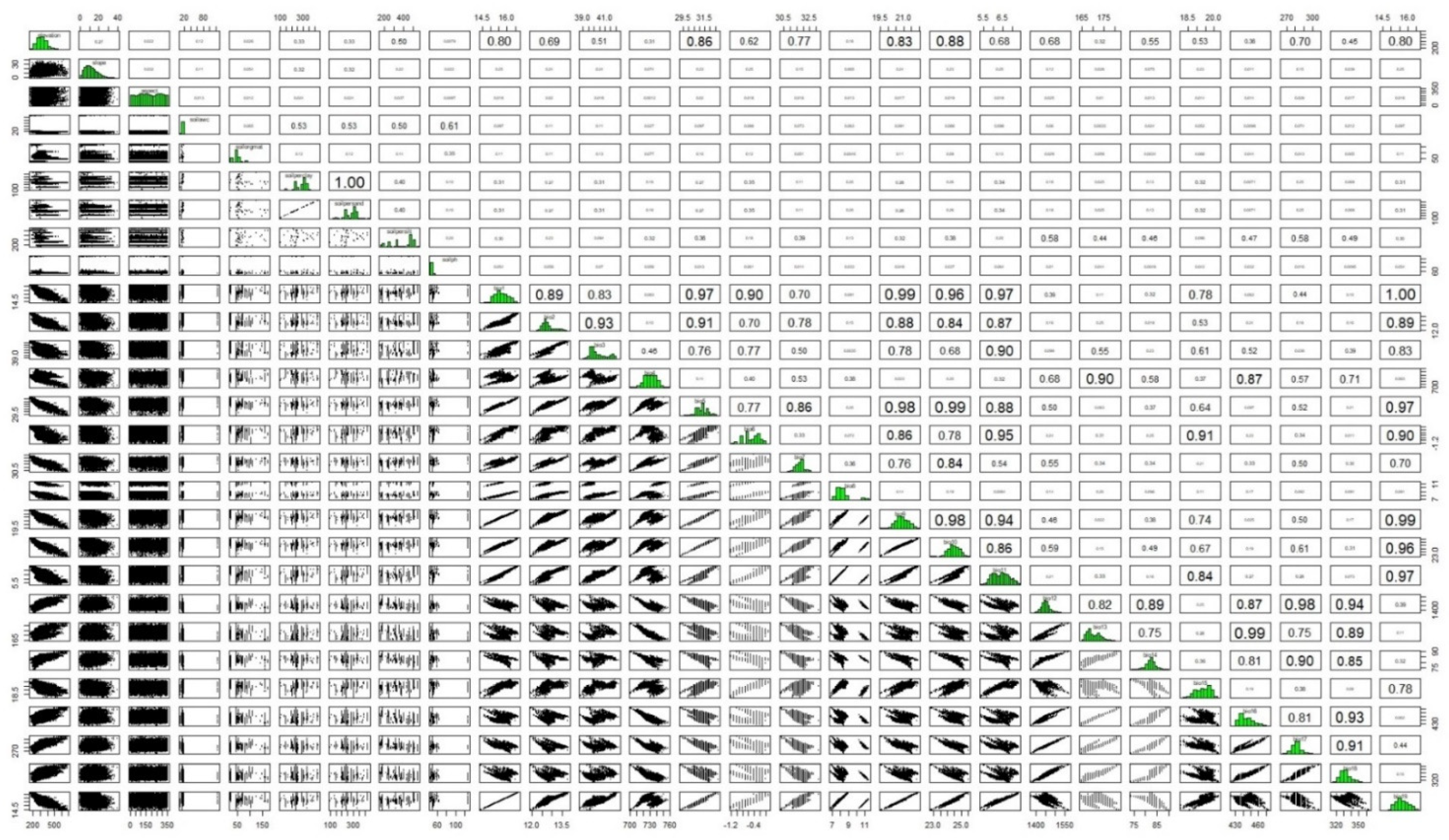
Sixteen environmental variables were eliminated based on Pearson’s r > 0.7 and VIF > 10, leaving 12 variables to be used in the models (Table 1).
The average AUC score was 0.99 for MaxEnt model (
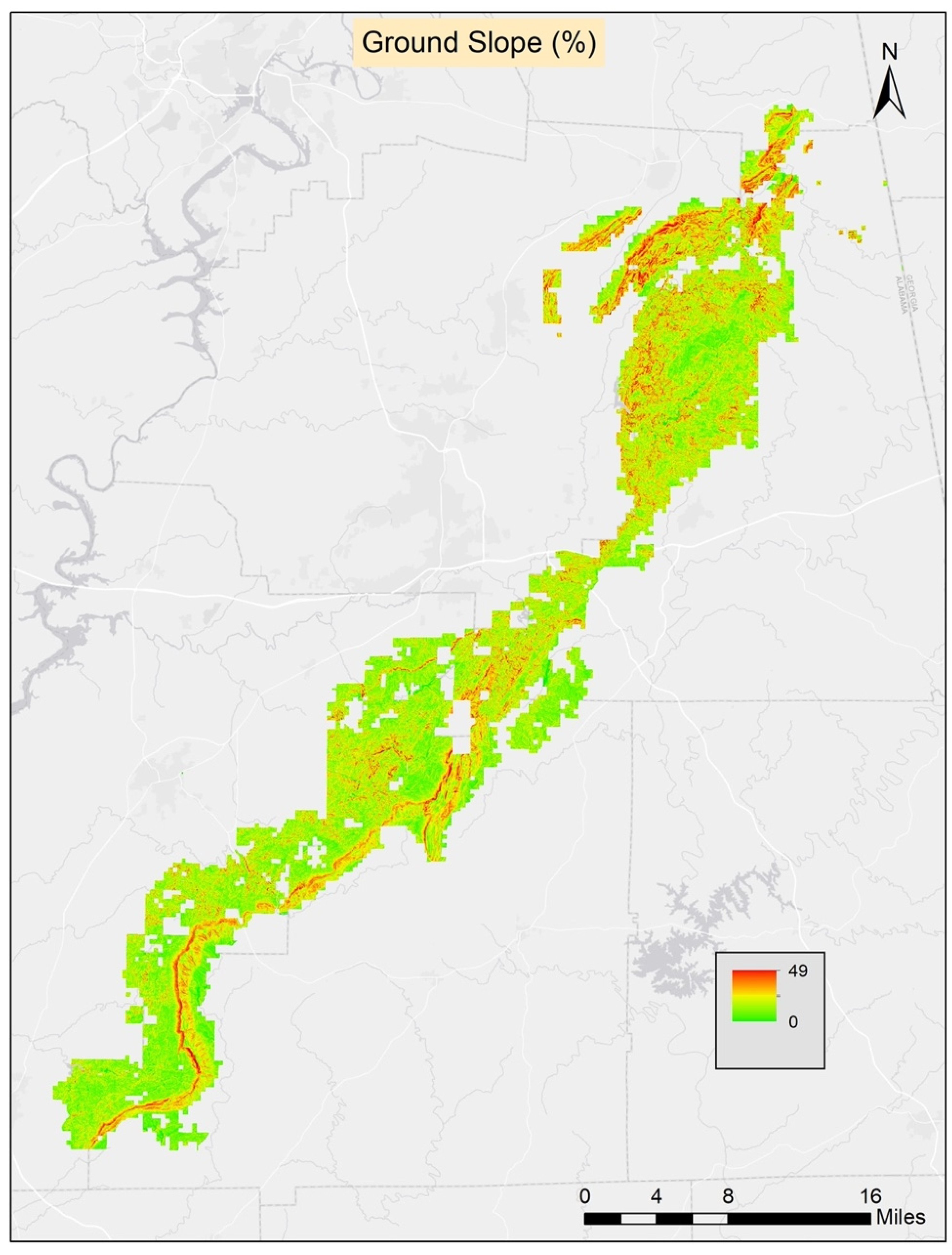
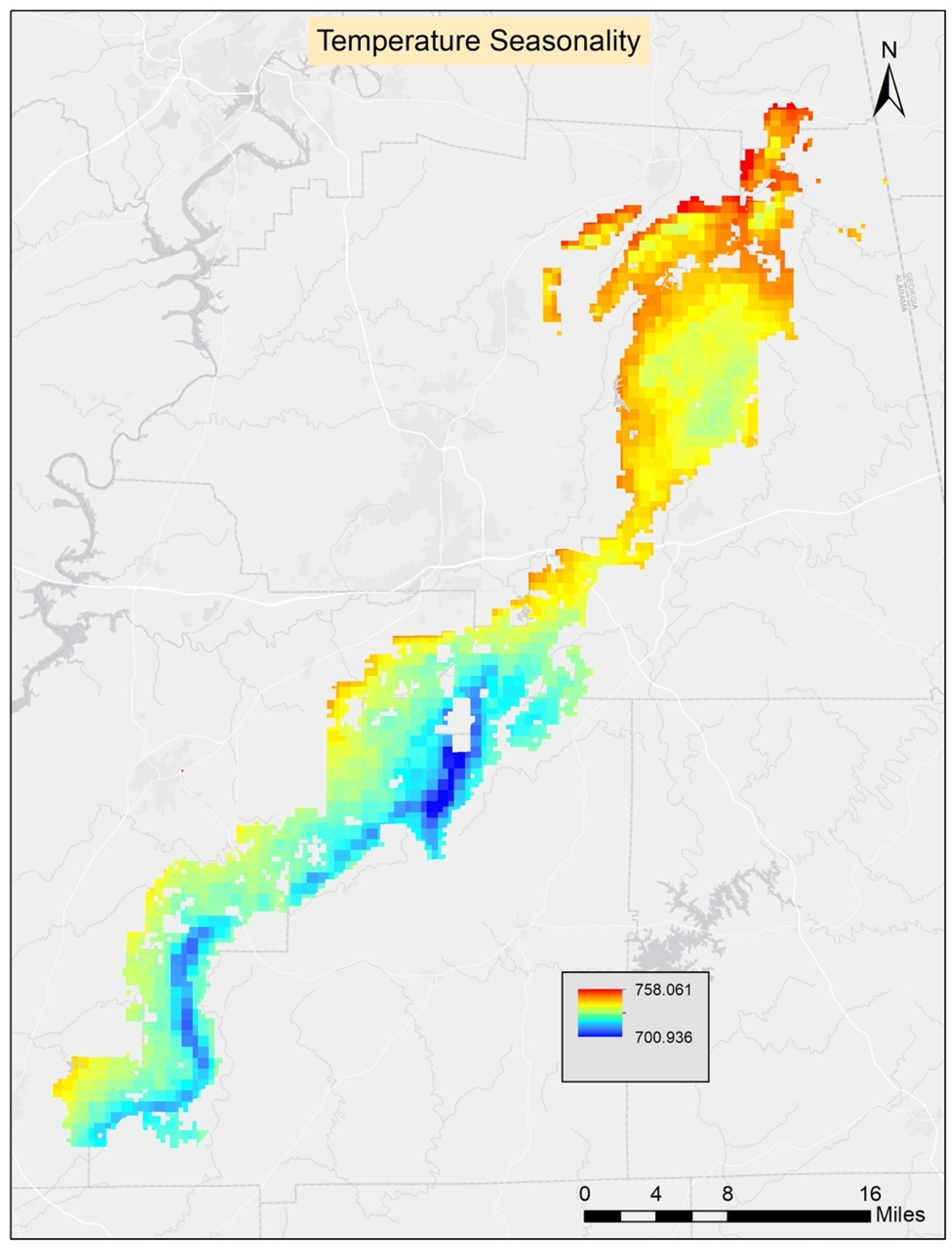
Table 2). The ground slope had the highest contribution to the model. The second highest contributing variable was Bio4 (temperature seasonality), and the third was Bio8 (mean temperature of the wettest quarter). The least contributing variables were aspect, soil available water content, and soil pH. The threshold average score for the 10 runs was found to be 0.51 and it was applied to generate the prediction map.
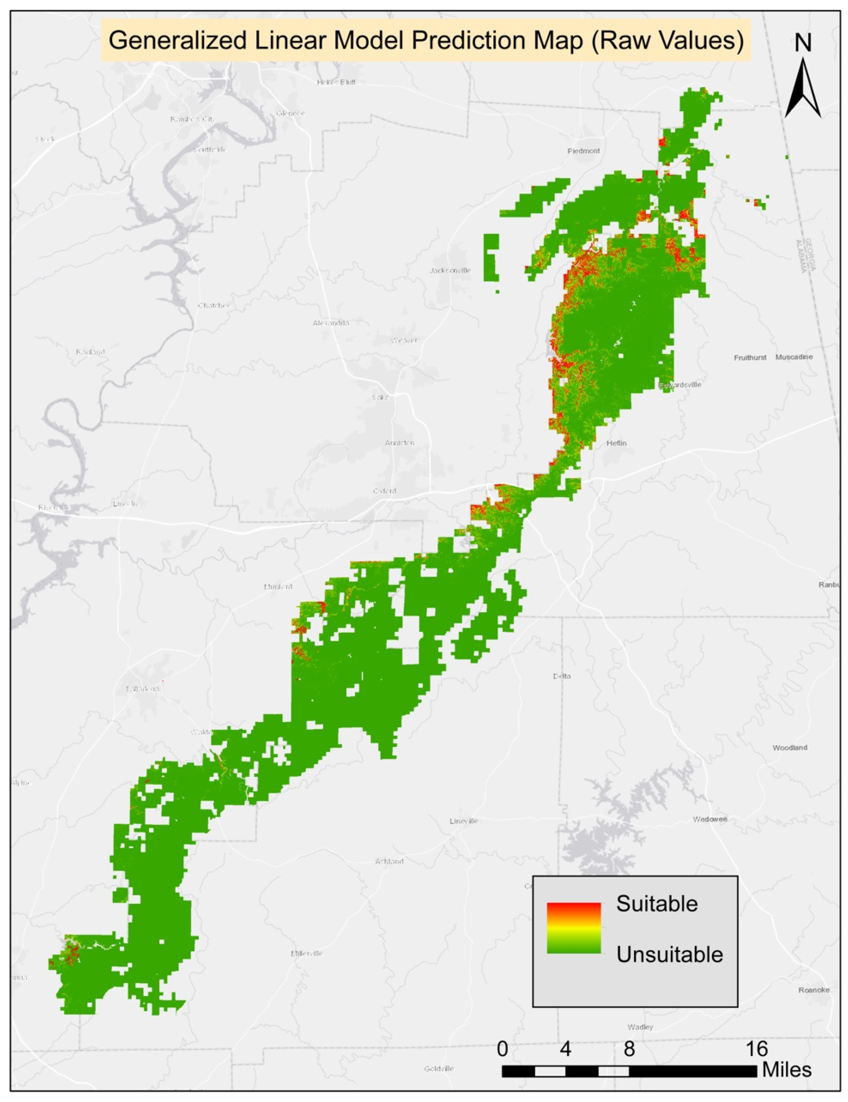
The best GLM model included seven environmental variables: ground slope, soil percent silt, Bio4 (temperature seasonality), Bio8 (mean temperature of the wettest quarter), soil available water content, soil percent clay, and elevation. However, only four variables had significant coefficients at p < 0.05, including ground slope, Bio4 (temperature seasonality), soil percent clay, and soil available water content. The threshold score for the best model was 0.15 and it was used to generate the final suitability map. Based on the best model, the AUC score was 0.96 (Table 2).
The best GAM model included five environmental variables: elevation, ground slope, soil percent clay, Bio4 (temperature seasonality), and Bio8 (mean temperature of the wettest quarter). Based on ANOVA parametric effects for the variables in the best model, all were significant except Bio4 (temperature seasonality). Based on ANOVA for nonparametric effects, Bio4 (temperature seasonality) and Bio8 (mean temperature of the wettest quarter) were found to be significant; however, elevation, ground slope, and soil percent clay were insignificant for nonparametric effects. The threshold score for the best model was 0.42 and it was applied to generate the final prediction map. The best GAM model AUC score was 0.98 (Table 2).
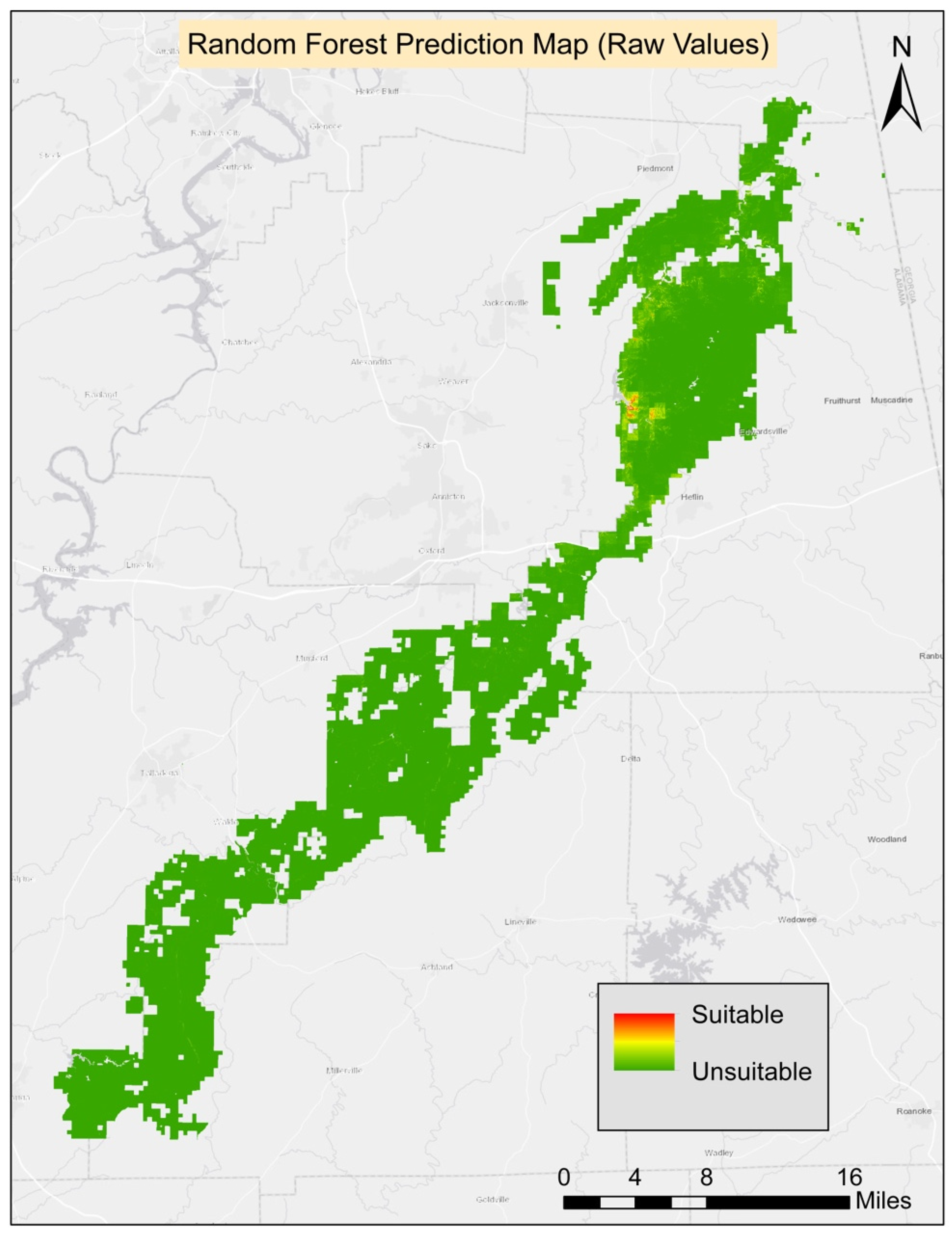
All 10 runs of RF were averaged, and they were evaluated to generate the final prediction maps and the AUC score was used to evaluate the model’s success. The average AUC score was 0.99 (Table 2). All 12 variables which were selected after the correlation check were used in the RF modeling process. The ground slope was the most contributive variable in the model followed by elevation and Bio4 (temperature seasonality). The least contributive variables were soil organic material, soil pH, and aspect. The threshold average score for the 10 runs was 0.39 and it was applied to generate the final prediction map.
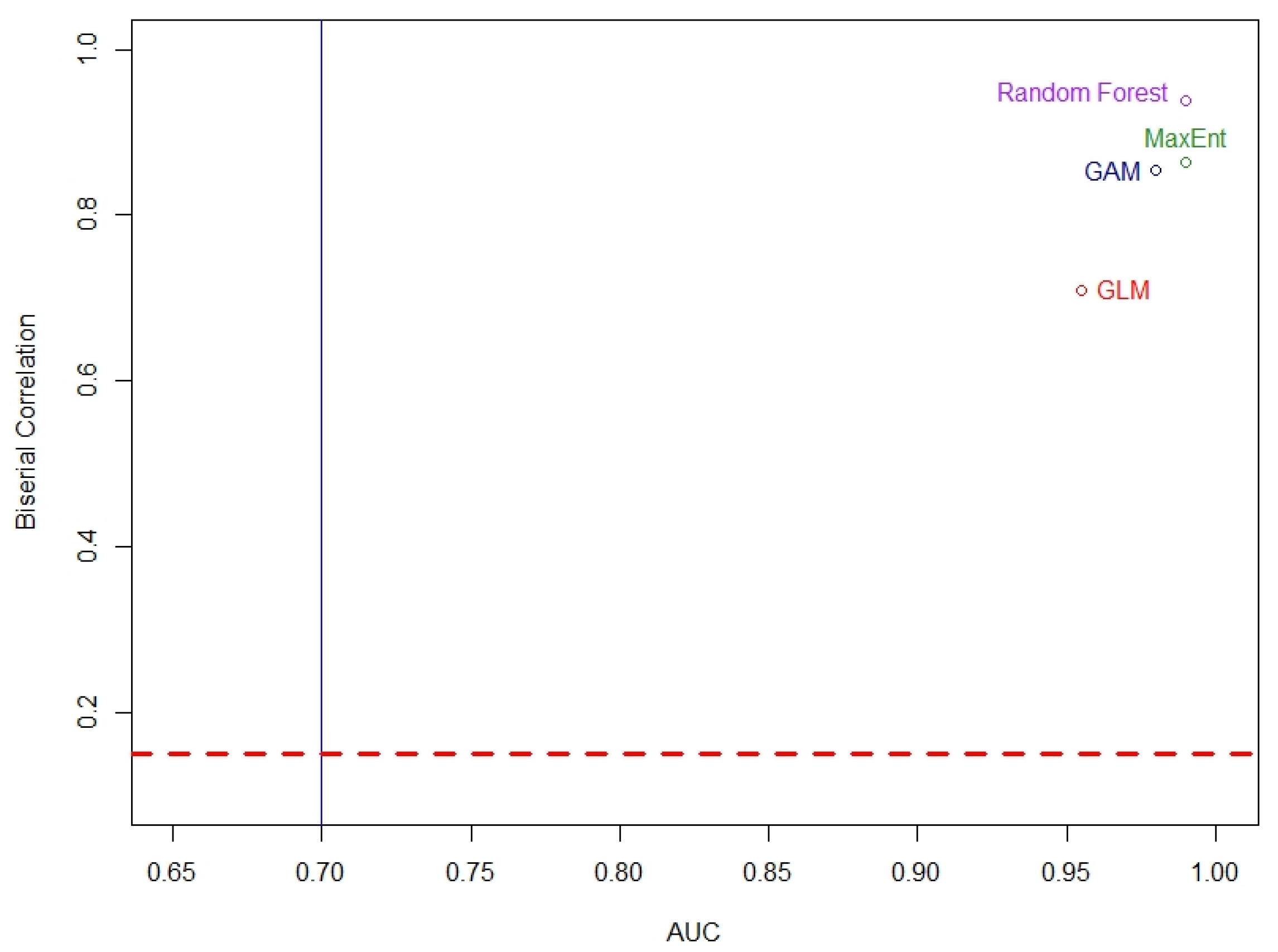
Based on the evaluation of all modeling approaches, the highest AUC score was 0.99 for the MaxEnt and RF analyses. The lowest AUC score was 0.96 for the GLM (Table 2), suggesting that the models were generally successful in classifying presence and pseudo-absence data for turkeybeard on the TNF with the given environmental variables. Based on the point-biserial correlation evaluation, the prediction performances for each model were found to be good. The lowest prediction performance was 0.71 for GLM, and the highest score was 0.94 for the RF (Table 2). The AUC and biserial correlation relation are given in Figure 2. Given both of these metrics (AUC and biserial correlation), the average of 10 runs of the RF model seemed to produce slightly better results for classifying presence and pseudo-absence data for turkeybeard on the TNF. The ground slope and elevation variables were the most important of the 12 variables used in the RF model runs. The other three models also used these two variables, but fewer of the other 10 variables because they were found to neither be statistically significant nor contributive to model results.
Based on our modeling process 97.01% (92,428.2 ha) of the land was assigned a predicted value (presence or absence). The remaining 2.99% (2847.8 ha) contained NODATA values as a result of missing values in one or more environmental data layers. Of the four models, the highest suitable area was 2979.2 ha (0.92%) using GLM predictions. The lowest amount of suitable area predicted was 225.9 ha (0.24%) of the TNF using RF (Table 3). The final habitat map was generated from the composite of four methods. All four models agreed on 159.57 ha (0.17%) of suitable habitat for turkeybeard. The prediction area from the agreement of three models was 310.05 ha (0.34%), 348.84 ha (0.38%) from two models, 2293.74 ha (2.48%) from a single model. The known presence locations comprise 2.62 ha; therefore, nearly 157 ha (159.57 ha–2.62 ha) of new potentially suitable locations are suggested based on suitable areas agreed on by all four models. The suitability maps for MaxEnt, GLM, GAM, and RF processes can be found in Appendix A.
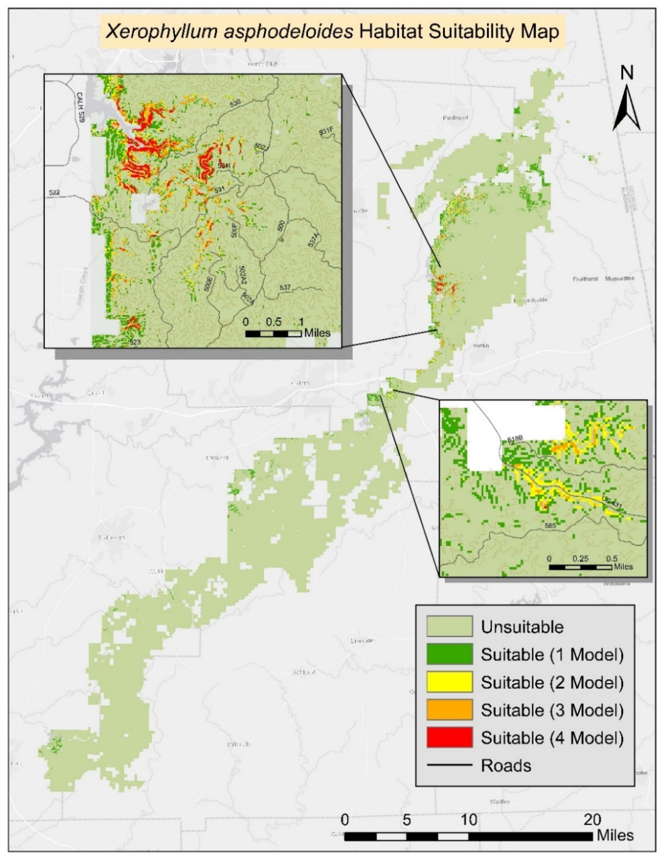
The final prediction map shows the most likely suitable areas in TNF represented by areas where all models agree (Figure 3). Based on the final suitability prediction map, the most highly suitable areas are mostly located in the same geographical areas as the already known populations. Most of the likely suitable locations are also located in the northern portion of the national forest. Suitable areas resulting from the combination of the four model outputs include the already known locations of turkeybeard.
Across all four methods, the most highly contributing (MaxEnt, RF) and significant (GLM, GAM) variable was ground slope. Furthermore, the Bio4 (temperature seasonality) variable was found to be highly contributive for the GLM and MaxEnt models and the elevation variable was found to be highly contributive for the GAM and RF models. Otherwise, the composition of each model’s significant or highest contributing variables was different. The five highest contributive variables of all four models can be found in Appendix A.

4. Discussion

The results indicate that using a small sample size for MaxEnt, GLM, GAM, and RF models can provide adequate habitat prediction results. As expected, the predictions of the suitable areas across the whole of the TNF were very low, ranging from just 0.24% of the area predicted by RF to 3.22% of the area predicted by GLM. The potentially suitable area that represents where all models agree, from the ensemble modeling effort, is only 0.17% of the TNF (159.57 ha). One of the most important limitations of this study was the presence of data for the species (only 22 sites). Turkeybeard species are located in 10 states, but each state has very low occurrences due to the species’ rareness. Only 22 occurrence locations were available from the TNF to generate the potentially suitable areas of the species. Based on the literature, sample size effects become less critical above 50 presences, even though some studies claim that some complex methods (MaxEnt) can effectively function with a small sample size [17,52,53,54]. Guisan et al. [17] also advise using 20 to 50 presence locations. However, Hernandez et al. [41] claimed that MaxEnt modeling can produce useful results with a sample size as small as five occurrences, yet the sample size can still have a profound impact on the predicted probability [55]. These issues are important as our small sample size may have led to overfitting the models. Further, the proportion of background (pseudo-absence) points may have led to biases in the results.
Another limitation of this study was the geographical distribution of the occurrences. When building a model, it is important to incorporate as many geographically diverse samples as possible [55]. The clustering of turkeybeard occurrence sites in a fairly limited geographic area resulted in a small area being predicted suitable. The models seemed to be able to discriminate between the environmental characteristics of the clustered locations of known turkeybeard and the random (pseudo-absence) points distributed across the more highly variable geography of the whole TNF. However, while similar, the outcomes (potential highly suitable habitat) from the four models were diverse enough to suggest caution is needed in preserving areas that were identified as potentially containing turkeybeard; proposed habitat areas will need to be examined for the presence of turkeybeard.
The first known study to predict habitat suitability for the turkeybeard was conducted by Bourg et al. [3]. They conducted their research in Virginia using 24 population occurrences of turkeybeard. For their analyses, they used elevation, slope, aspect, forest type, six soil variables (composition, depth, drainage, pH, fertility, and water capacity), and fire frequency variables. Their models did not include climate variables, but their models included fire frequency variables, unlike our research. They used the classification and regression tree (CART) modeling using GIS, and generally, their modeling effort was successful at defining suitable habitats for turkeybeard. They found that four variables (elevation, slope, forest type, fire frequency) were major determinants for estimating turkeybeard distribution. Our studies agree on the importance of slope, and some agree on elevation, but we did not consider fire frequency and forest type which may be important to consider in future models. Elevation likely did not show up as very important in our work due to either a lack of sufficient variability in those gradients across the TNF, or a lack of sufficient sample locations to successfully identify a relationship over random variability. Our study shows that ground slope is the most contributive variable among all models. Elevation is the second highest contributive variable for GAM and RF models, whereas Bio4 (temperature seasonality) is the second highest contributive variable for the MaxEnt and GLM models. This shows some initial agreement among the four models.
Several other studies found the climate and soil conditions important for estimating plant abundance and distribution [56,57,58]. Based on this guidance, we included climate and soil variables in our models. Chauvier et al. [59] found that the most important environmental factors for the distribution of the plant species involved the climate. In this work, climate variables were also found effective, but soil variables produced insignificant effects. For further study, if more geographically diverse populations of turkeybeard are located, it may help isolate the effects of soil components on the species distribution. Knowledge of understory herb distribution may have further informed this analysis. Yet, given the raster GIS databases available to this study, and the inability to access the study area due to COVID restrictions placed on access to it by the U.S. government, the inclusion of an understory herb database—or field data that represent understory herb distributions—was not possible. The TNF is a very diverse landscape with stands of trees of varying canopy closure. However, given our prior experience in working on this landscape, only a field-based sample could have been collected (given enough time and resources); a remotely sensed (or interpolated) database representing understory herbs would have been elusive.
As with efforts to model any rare species, the identification of new occurrence locations in new areas (not proximal to known sites), would offer the greatest improvement for predicting likely suitable areas. Turkeybeard is one of the few known fire-adapted forest understory plant species, and fire has been shown to have a significant positive effect on the reproductive performance of turkeybeard [4]. Based on this importance, future modeling efforts for turkeybeard habitat suitability should consider including fire frequency or fire history variables. In the future, studies such as this may also benefit from including socio-cultural considerations in addition to environmental gradients for describing turkeybeard habitat suitability. For instance, in field observations, turkeybeard was located near hilltops in sheltered areas, suggesting that its location may be related to structures used by ancient Native American peoples who may have protected this species around their living areas and used it as building and fire-starting materials. While we found no readily available evidence for this at present, an investigation into the socio-cultural history of the region may provide clues.
Species habitat suitability models can be used to model rare species in support of forest management goals if appropriate caution is used when interpreting results. Managers may also use these models to identify and plan for enhancements to the distribution of important species in their landscape. It may also be useful to the decision-making process to model potential plant responses to future climate change. This preliminary modeling effort can be useful for identifying new turkeybeard population locations in the TNF and for better understanding the relationship between turkeybeard and environmental gradients that likely influence its distribution.

5. Conclusions

This study represents the first effort to model potentially suitable habitats for the rare and threatened turkeybeard in the southern part of its range. This study’s findings show that the distribution of turkeybeard is highly related to ground slope and temperature seasonality. Excluding known locations, the new areas the models indicated as potentially suitable for turkeybeard were very small in size and extent. However, based on the very low known presence of the species in the study area, this was expected. To improve models, surveys of turkeybeard populations across a larger range of soil types throughout the TNF would be useful. Prediction maps from this study can be used to guide future field surveys and improve the detection of unknown populations in the study area. For this rare plant species field survey, an ecologically informed meander search technique can be used. This study is also important for further forest management of the TNF and to help schedule forest management activities. There are currently no apparent protection plans for turkeybeard species in the TNF management plan, but a protection plan could be developed in the future if interest exists. Knowledge gained from this research can be used to establish and implement habitat management strategies for turkeybeard across the TNF. Further, a focus might be applied to this rare species to help understand the potential impacts of climate change, by modeling suitable habitat locations using various climate change scenarios. Incorporating habitat suitability modeling into management planning efforts may therefore facilitate the selection of sustainable forest management practices.

Author Contributions

Conceptualization, V.B. and P.B.; methodology, V.B., P.B. and N.N.; software, V.B. and K.A.H.; validation, V.B., P.B. and N.N.; formal analysis, V.B., P.B. and N.N.; resources, V.B. and J.S. (Jonathan Stober); data curation, V.B., K.A.H. and K.M.; writing—original draft preparation, V.B.; writing—review and editing, V.B., P.B., N.N., J.S. (Jacek Siry), K.M., K.A.H. and J.S. (Jonathan Stober); visualization, V.B.; supervision, P.B. All authors have read and agreed to the published version of the manuscript.

Funding

This research received no external funding.

Institutional Review Board Statement

Not applicable.

Informed Consent Statement

Not applicable.

Data Availability Statement

The data presented in this study are available on request from the corresponding author.

Acknowledgments

This work was supported by the Republic of Turkey, Ministry of National Education and the Warnell School of Forestry and Natural Resources at the University of Georgia. We would like to thank United States Forest Service for their data and assistance.

Conflicts of Interest

The authors declare no conflict of interest.

Appendix A

Figure A1. Correlation matrix for all environmental variables.
Forests 13 00490 g0a1
Table A1. Detailed explanation of bioclimate variables and used input variables in the model.
CodeExplanation
BIO1Annual Mean Temperature
BIO2Mean Diurnal Range (Mean of monthly (max temp-min temp))
BIO3Isothermality (BIO2/BIO7) (×100)
BIO4Temperature Seasonality (standard deviation ×100)
BIO5Max Temperature of Warmest Month
BIO6Min Temperature of Coldest Month
BIO7Temperature Annual Range (BIO5-BIO6)
BIO8Mean Temperature of Wettest Quarter
BIO9Mean Temperature of Driest Quarter
BIO10Mean Temperature of Warmest Quarter
BIO11Mean Temperature of Coldest Quarter
BIO12Annual Precipitation
BIO13Precipitation of Wettest Month
BIO14Precipitation of Driest Month
BIO15Precipitation Seasonality (Coefficient of Variation)
BIO16Precipitation of Wettest Quarter
BIO17Precipitation of Driest Quarter
BIO18Precipitation of Warmest Quarter
BIO19Precipitation of Coldest Quarter
SlopeGround Slope
AspectAspect
ElevationElevation
SoilawcSoil Water Content
SoilorgmatSoil Organic Material
SoilperclaySoil Percentage of Clay
SoilpersandSoil Percentage of Sand
SoilpersiltSoil Percentage of Silt
SoilphSoil PH
Table A2. Variable contribution and sign of coefficient for the Generalized Linear Model.
VariablePercent Contribution (Sign of Coefficient)
Ground slope22.7 (+)
Temperature seasonality 16.6 (+)
Soil percentage of clay13.0 (+)
Soil water content10.5 (+)
Elevation7.8 (−)
Table A3. Variable contribution and sign of coefficient for the Generalized Additive Model.
VariablePercent Contribution (Sign of Coefficient)
Ground slope60.0 (+)
Elevation24.3 (−)
Soil percentage of clay11.5 (+)
Mean temperature of wettest quarter3.4 (+)
Temperature seasonality 0.71 (−)
Table A4. Variable contribution and sign of coefficient for the MaxEnt model.
VariablePercent Contribution (Sign of Coefficient)
Ground slope41 (+)
Temperature seasonality 19 (+)
Mean temperature of wettest quarter 16 (+)
Soil percentage of silt9 (+)
Elevation8 (+)
Table A5. Variable contribution for Random Forest model.
VariablePercent Contribution
Ground Slope19
Elevation13
Temperature seasonality12
Isothermality 12
Mean temperature of wettest quarter 9
Figure A2. Xerophyllum asphodeloides (turkeybeard) Generalized Linear Model habitat suitability map.
Forests 13 00490 g0a2
Figure A3. Xerophyllum asphodeloides (turkeybeard) Generalized Additive Model habitat suitability map.
Forests 13 00490 g0a3
Figure A4. Xerophyllum asphodeloides (turkeybeard) MaxEnt model habitat suitability map.
Forests 13 00490 g0a4
Figure A5. Xerophyllum asphodeloides (turkeybeard) Random Forest model habitat suitability map.
Forests 13 00490 g0a5
Figure A6. Ground slope for Talladega National Forest.
Forests 13 00490 g0a6
Figure A7. Temperature seasonality for Talladega National Forest.
Forests 13 00490 g0a7

References

  1. Nuttall, T. The Genera of North American Plants and a Catalogue of the Species, to the Year 1817; D. Heartt: Philadelphia, PA, USA, 1818; Volume 1, pp. 1500–1926. [Google Scholar]
  2. Fernald, M.L. Gray’s Manual of Botany, 8th ed.; American Book Company: New York, NY, USA, 1950. [Google Scholar]
  3. Bourg, N.A.; McShea, W.J.; Gill, D.E. Putting a CART before the search: Successful habitat prediction for a rare forest herb. Ecology 2005, 86, 2793–2804. [Google Scholar] [CrossRef]
  4. Bourg, N.A.; Gill, D.E.; McShea, W.J. Fire and canopy removal effects on demography and reproduction in turkeybeard (Xerophyllum asphodeloides), a fire-dependent temperate forest herb. J. Sustain. For. 2015, 34, 71–104. [Google Scholar] [CrossRef]
  5. Keener, B.R.; Diamond, A.R.; Davenport, L.J.; Davison, P.G.; Ginzbarg, S.L.; Hansen, C.J.; Major, C.S.; Spaulding, D.D.; Triplett, J.K.; Woods, M. Alabama Plant Atlas. University of West Alabama, Livingston, AL. Available online: http://floraofalabama.org/Plant.aspx?id=4502 (accessed on 9 August 2021).
  6. United States Department of Agriculture. Plant Profile. United States Department of Agriculture, Forest Service, Washington, D.C. Available online: https://plants.usda.gov/core/profile?symbol=XEAS (accessed on 16 July 2020).
  7. Center for Plant Conservation. Plant Profile—Xerophyllum asphodeloides. Center for Plant Conservation, Escondido, CA. Available online: https://saveplants.org/plant-profile/?CPCNum=6634 (accessed on 16 July 2020).
  8. Pecchi, M.; Marchi, M.; Burton, V.; Giannetti, F.; Moriondo, M.; Bernetti, I.; Bindi, M.; Chirici, G. Species distribution modelling to support forest management. A literature review. Ecol. Model. 2019, 411, 108817. [Google Scholar] [CrossRef]
  9. Pecchi, M.; Marchi, M.; Giannetti, F.; Bernetti, I.; Bindi, M.; Moriondo, M.; Maselli, F.; Fibbi, L.; Corona, P.; Travaglini, D.; et al. Reviewing climatic traits for the main forest tree species in Italy. iForest 2019, 12, 173–180. [Google Scholar] [CrossRef] [Green Version]
  10. Edenius, L.; Mikusiński, G. Utility of habitat suitability models as biodiversity assessment tools in forest management. Scand. J. For. Res. 2006, 21, 62–72. [Google Scholar] [CrossRef]
  11. Liu, S.; Lin, Y.; Zhang, Y.; Guo, Z.; Zhang, L.; Li, C.; Wang, J. Landscape ecology contributions to forestry and forest management in China: Progresses and research needs. In Landscape Ecology in Forest Management and Conservation; Li, C., Lafortezza, R., Chen, J., Eds.; Springer: Berlin/Heidelberg, Germany, 2011; pp. 22–45. [Google Scholar]
  12. United States Department of Agriculture. Forest Service Home. Forest Management. About Us. United States Department of Agriculture, Forest Service, Washington, D.C. Available online: https://www.fs.fed.us/forestmanagement/aboutus/ecoperspective.shtml#:~:text=The%20overriding%20objective%20of%20the,of%20forests%20through%20their%20actions (accessed on 17 July 2020).
  13. Giles, R.H., Jr. Wildlife Management; W.H. Freeman: San Francisco, CA, USA, 1978. [Google Scholar]
  14. United States Fish and Wildlife Service. Standards for the Development of Habitat Suitability Index Models; Release No. 1-81,103 ESM; United States Fish and Wildlife Service: Washington, DC, USA, 1981.
  15. Kliskey, A.D.; Lofroth, E.C.; Thompson, W.A.; Brown, S.; Schreier, H. Simulating and evaluating alternative resource-use strategies using GIS-based habitat suitability indices. Landsc. Urban Plan. 1999, 45, 163–175. [Google Scholar] [CrossRef]
  16. Wiens, J.A. Predicting species occurrences: Progress, problems, and prospects. In Predicting Species Occurrence: Issues of Accuracy and Scale; Scott, J.M., Heglund, P.J., Morrison, M.L., Haufler, J.B., Raphael, M.G., Wall, W.A., Samson, F.B., Eds.; Island Press: Washington, DC, USA, 2002; pp. 739–749. [Google Scholar]
  17. Guisan, A.; Thuiller, W.; Zimmermann, N.E. Habitat Suitability and Distribution Models: With Applications in R; Cambridge University Press: Cambridge, UK, 2017. [Google Scholar]
  18. McCullagh, P.; Nelder, J.A. Generalized Linear Models; Chapman and Hall: London, UK, 1989. [Google Scholar]
  19. Breiman, L.; Friedman, J.H.; Olshen, R.A.; Stone, C.J. Classification and Regression Trees; Wadsworth International Group: Belmont, CA, USA, 1984. [Google Scholar]
  20. Breiman, L. Random forests. Mach. Learn. 2001, 45, 5–32. [Google Scholar] [CrossRef] [Green Version]
  21. Rosenblatt, F. The perceptron: A probabilistic model for information storage and organization in the brain. Psychol. Rev. 1958, 65, 386–408. [Google Scholar] [CrossRef] [PubMed] [Green Version]
  22. Hastie, T.; Tibshirani, R. Exploring the nature of covariate effects in the proportional hazards model. Biometrics 1990, 46, 1005–1016. [Google Scholar] [CrossRef]
  23. Phillips, S.J.; Anderson, R.P.; Schapire, R.E. Maximum entropy modeling of species geographic distributions. Ecol. Model. 2006, 190, 231–259. [Google Scholar] [CrossRef] [Green Version]
  24. United States Department of Agriculture. Establishment and Modification of National Forest Boundaries and National Grasslands. A Chronological Record 1891–2012; FS-612; United States Department of Agriculture: Washington, DC, USA, 2012.
  25. University of Alabama Department of Geography. Alabama Ecoregions. Available online: http://alabamamaps.ua.edu/Interactive%20Maps/Physical/Ecoregions.html (accessed on 6 December 2020).
  26. University of Alabama Department of Geography. Alabama Historical Climate Data. Available online: http://alabamamaps.ua.edu/Interactive%20Maps/Climate/WeatherStations.html (accessed on 28 January 2021).
  27. Stober, J.; Merry, K.; Bettinger, P. Analysis of fire frequency on the Talladega National Forest, USA, 1998–2018. Int. J. Wildland Fire 2020, 29, 919–925. [Google Scholar] [CrossRef]
  28. Lee, T.; Bettinger, P.; Cieszewski, C.J.; Gutierrez Garzon, A.R. The applicability of recreation-grade GNSS receiver (GPS watch, Suunto Ambit Peak 3) in a forested and an open area compared to a mapping-grade receiver (Trimble Juno T41). PLoS ONE 2020, 15, e0231532. [Google Scholar] [CrossRef] [PubMed]
  29. Fick, S.E.; Hijmans, R.J. WorldClim 2: New 1 km spatial resolution climate surfaces for global land areas. Int. J. Climatol. 2017, 37, 4302–4315. [Google Scholar] [CrossRef]
  30. United States Department of Agriculture. National Elevation Dataset 30 m. United States Department of Agriculture, Natural Resources Conservation Service. Washington, D.C. 2014. Available online: http://datagateway.nrcs.usda.gov/ (accessed on 16 March 2022).
  31. United States Department of Agriculture. SSURGO-Web Soil Survey 3.3. Washington, D.C. 2019. Available online: https://websoilsurvey.sc.egov.usda.gov/app/homepage.htm (accessed on 16 March 2022).
  32. Menard, S. Applied Logistic Regression Analysis, 2nd ed.; Sage Publishing: Thousand Oaks, CA, USA, 2002. [Google Scholar]
  33. Green, R.H. Sampling Design and Statistical Methods for Environmental Biologists; John Wiley & Sons: New York, NY, USA, 1979. [Google Scholar]
  34. Harrell, F.E. Resampling, validating, describing, and simplifying the model. In Regression Modeling Strategies; Harrell, F.E., Ed.; Springer: New York, NY, USA, 2001; pp. 87–103. [Google Scholar]
  35. Guisan, A.; Lehmann, A.; Ferrier, S.; Austin, M.; Overton, J.M.C.; Aspinall, R.; Hastie, T. Making better biogeographical predictions of species’ distributions. J. Appl. Ecol. 2006, 43, 386–392. [Google Scholar] [CrossRef]
  36. Hair, J.F.; Anderson, R.E.; Tatham, R.L.; Black, W.C. Multivariate Data Analysis, 5th ed.; Prentice Hall: Upper Saddle River, NJ, USA, 1998. [Google Scholar]
  37. Chatterjee, S.; Hadi, A.S. Regression Analysis by Example; John Wiley & Sons: Hoboken, NJ, USA, 2006. [Google Scholar]
  38. Hirzel, A.H.; Helfer, V.; Metral, F. Assessing habitat-suitability models with a virtual species. Ecol. Model. 2001, 145, 111–121. [Google Scholar] [CrossRef] [Green Version]
  39. Guisan, A.; Edwards, T.C., Jr.; Hastie, T. Generalized linear and generalized additive models in studies of species distributions: Setting the scene. Ecol. Model. 2002, 157, 89–100. [Google Scholar] [CrossRef] [Green Version]
  40. Yee, T.W.; Mitchell, N.D. Generalized additive models in plant ecology. J. Veg. Sci. 1991, 2, 587–602. [Google Scholar] [CrossRef]
  41. Hernandez, P.A.; Graham, C.H.; Master, L.L.; Albert, D.L. The effect of sample size and species characteristics on performance of different species distribution modeling methods. Ecography 2006, 29, 773–785. [Google Scholar] [CrossRef]
  42. Phillips, S.J.; Dudík, M. Modeling of species distributions with Maxent: New extensions and a comprehensive evaluation. Ecography 2008, 31, 161–175. [Google Scholar] [CrossRef]
  43. Benito, B.M.; Martínez-Ortega, M.M.; Muñoz, L.M.; Lorite, J.; Peñas, J. Assessing extinction-risk of endangered plants using species distribution models: A case study of habitat depletion caused by the spread of greenhouses. Biodivers. Conserv. 2009, 18, 2509–2520. [Google Scholar] [CrossRef]
  44. Garzón, M.B.; Blazek, R.; Neteler, M.; de Dios, R.S.; Ollero, H.S.; Furlanello, C. Predicting habitat suitability with machine learning models: The potential area of Pinus sylvestris L. in the Iberian Peninsula. Ecol. Model. 2006, 197, 383–393. [Google Scholar] [CrossRef]
  45. Shataee, S.; Kalbi, S.; Fallah, A.; Pelz, D. Forest attribute imputation using machine-learning methods and ASTER data: Comparison of k-NN, SVR and random forest regression algorithms. Int. J. Remote Sens. 2012, 33, 6254–6280. [Google Scholar] [CrossRef]
  46. Valavi, R.; Guillera-Arroita, G.; Lahoz-Monfort, J.; Elith, J. Predictive performance of presence-only species distribution models: A benchmark study with reproducible code. Ecol. Monogr. 2022, 92, e01486. [Google Scholar] [CrossRef]
  47. Liu, C.; Berry, P.M.; Dawson, T.P.; Pearson, R.G. Selecting thresholds of occurrence in the prediction of species distributions. Ecography 2005, 28, 385–393. [Google Scholar] [CrossRef]
  48. Wei, B.; Wang, R.; Hou, K.; Wang, X.; Wu, W. Predicting the current and future cultivation regions of Carthamus tinctorius L. using MaxEnt model under climate change in China. Glob. Ecol. Conserv. 2018, 16, e00477. [Google Scholar]
  49. Swets, J.A. Measuring the accuracy of diagnostic systems. Science 1988, 240, 1285–1293. [Google Scholar] [CrossRef] [Green Version]
  50. Elith, J.; Graham, C.H.; Anderson, R.P.; Dudik, M.; Ferrier, S.; Guisan, A.; Hijmans, R.J.; Huettmann, F.; Leathwick, J.R.; Lehmann, A.; et al. Novel methods improve prediction of species’ distributions from occurrence data. Ecography 2006, 29, 129–151. [Google Scholar] [CrossRef] [Green Version]
  51. Varma, S. Preliminary Item Statistics Using Point-Biserial Correlation and p-Values; Educational Data Systems Inc.: Morgan Hill, CA, USA, 2006. [Google Scholar]
  52. Stockwell, D.R.; Peterson, A.T. Effects of sample size on accuracy of species distribution models. Ecol. Model. 2002, 148, 1–13. [Google Scholar] [CrossRef]
  53. Pearson, R.G.; Raxworthy, C.J.; Nakamura, M.; Townsend Peterson, A. Predicting species distributions from small numbers of occurrence records: A test case using cryptic geckos in Madagascar. J. Biogeogr. 2007, 34, 102–117. [Google Scholar] [CrossRef]
  54. Thibaud, E.; Petitpierre, B.; Broennimann, O.; Davison, A.C.; Guisan, A. Measuring the relative effect of factors affecting species distribution model predictions. Methods Ecol. Evol. 2014, 5, 947–955. [Google Scholar] [CrossRef]
  55. Li, Y.; Ding, C. Effects of sample size, sample accuracy and environmental variables on predictive performance of MaxEnt model. Pol. J. Ecol. 2016, 64, 303–312. [Google Scholar] [CrossRef]
  56. Walthert, L.; Meier, E.S. Tree species distribution in temperate forests is more influenced by soil than by climate. Ecol. Evol. 2017, 7, 9473–9484. [Google Scholar] [CrossRef] [PubMed]
  57. Chakraborty, D.; Jandl, R.; Kapeller, S.; Schueler, S. Disentangling the role of climate and soil on tree growth and its interaction with seed origin. Sci. Total Environ. 2019, 654, 393–401. [Google Scholar] [CrossRef] [PubMed]
  58. Buri, A.; Grand, S.; Yashiro, E.; Adatte, T.; Spangenberg, J.E.; Pinto-Figueroa, E.; Verrecchia, E.; Guisan, A. What are the most crucial soil variables for predicting the distribution of mountain plant species? A comprehensive study in the Swiss Alps. J. Biogeogr. 2020, 47, 1143–1153. [Google Scholar]
  59. Chauvier, Y.; Thuiller, W.; Brun, P.; Lavergne, S.; Descombes, P.; Karger, D.N.; Renaud, J.; Zimmermann, N.E. Influence of climate, soil, and land cover on plant species distribution in the European Alps. Ecol. Monogr. 2021, 91, e01433. [Google Scholar] [CrossRef]
Figure 1. Talladega National Forest and turkeybeard occurrence locations (from field observations). (Basemap sources: ESRI).
Forests 13 00490 g001
Figure 2. AUC and biserial correlation graph for all models. The red dashed line represents 0.15 value for good biserial correlation. The blue solid line represents 0.7 value for good AUC.
Forests 13 00490 g002
Figure 3. Xerophyllum asphodeloides (turkeybeard) habitat suitability map (Basemaps sources: ESRI).
Forests 13 00490 g003
Table 1. VIFs of the 12 variables that remain after elimination based on Pearson’s r and VIF scores.
VariablesVIF Scores
Elevation5.371157
Slope1.215588
Aspect1.029485
Soil available water content1.972491
Soil organic material2.019679
Soil percent clay1.902937
Soil percent silt2.991156
Soil percent pH2.450709
Bio3 (Isothermality)3.579550
Bio4 (Temperature seasonality)4.743466
Bio8 (Mean temperature of wettest quarter)1.605334
Bio15 (Precipitation seasonality)2.740790
Table 2. AUC and biserial correlation scores of all modeling methods.
ModelsAUCBiserial Correlation
MaxEnt0.990.86
GLM0.960.71
GAM0.980.85
RF0.990.94
Table 3. Suitable areas based on the models for the turkeybeard species in the Talladega National Forest.
ModelsArea (ha)Percent (%) of the TNF 1
MaxEnt682.650.74
GLM2979.183.22
GAM672.120.73
RF225.900.24
1 Talladega National Forest.
Publisher’s Note: MDPI stays neutral with regard to jurisdictional claims in published maps and institutional affiliations.

