
Effects of Mixture Mode on the Canopy Bidirectional Reflectance of Coniferous–Broadleaved Mixed Plantations

Abstract
:1. Introduction
2. Materials and Methods
2.1. Study Area
2.2. Data Acquisitions
2.3. Methods
2.3.1. The DART Model
2.3.2. The 3-PGmix Model
2.3.3. Parameterization for Simulation
2.3.4. Relationship Analysis
2.3.5. Spatial Scale Analysis
3. Results
3.1. Simulations of Sample Plots
3.2. Relationship between Canopy BRFs and Mixture Modes
3.2.1. The Effects of Mixing Proportions on Canopy BRFs
3.2.2. The Effects of Mixture Patterns on Canopy BRFs
3.3. The Effects of Solar-Viewing Geometries on Canopy BRFs
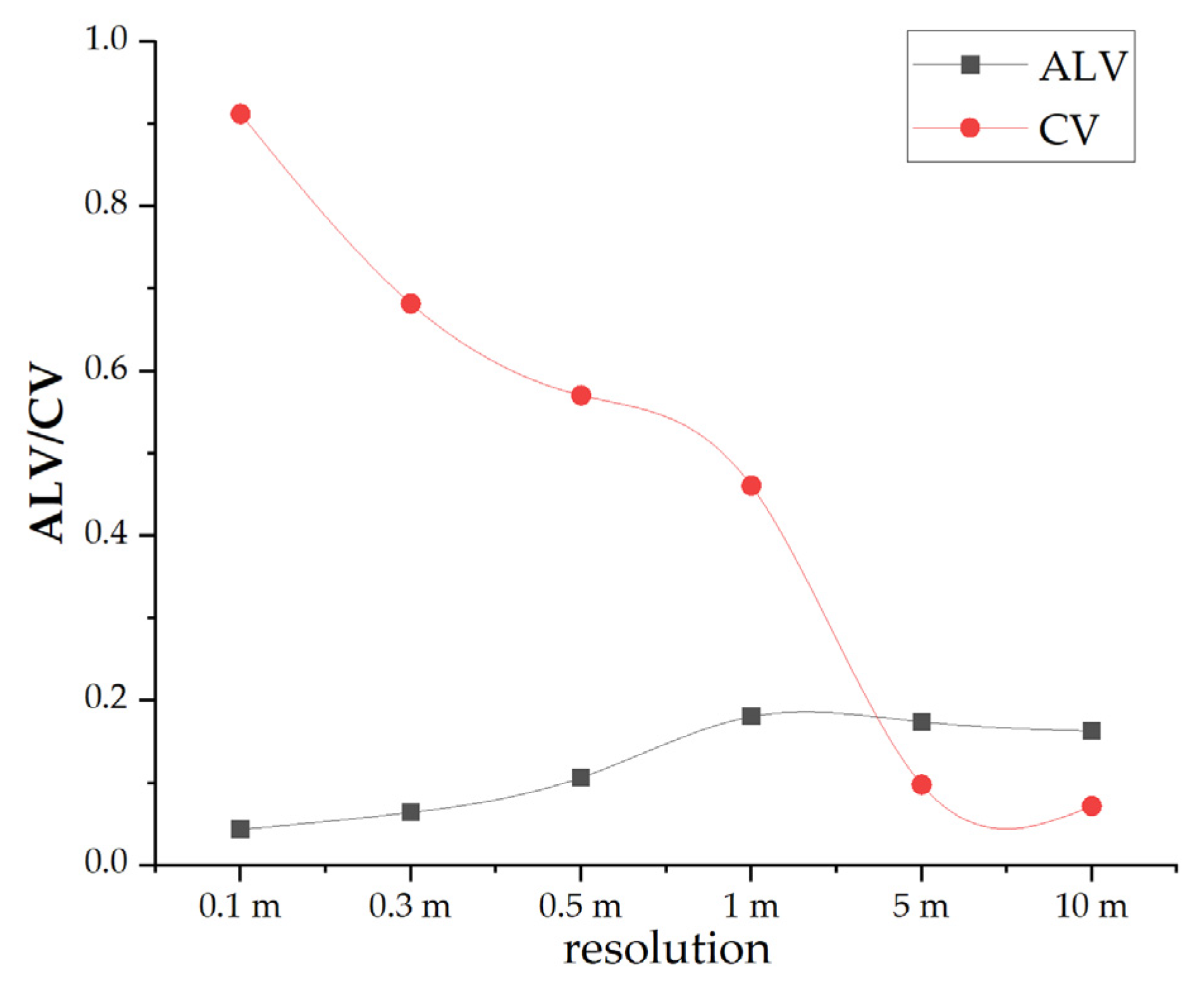
3.4. Optimal Spatial Resolution
4. Discussions
4.1. Influence of Mixture Modes on Simulated Canopy BRFs
4.2. Effects of Different Solar-Viewing Geometries on Canopy BRFs
4.3. Optimal Spatial Resolution
4.4. Suggestions for Future Research
5. Conclusions
Supplementary Materials
Author Contributions
Funding
Institutional Review Board Statement
Informed Consent Statement
Data Availability Statement
Acknowledgments
Conflicts of Interest
References
- National Forestry and Grassland Administration. China Forest Resources Report (2014–2018); China Forestry Publishing House: Beijing, China, 2019. [Google Scholar]
- Yu, G.; Chen, Z.; Piao, S.; Peng, C.; Ciais, P.; Wang, Q.; Li, X.; Zhu, X. High carbon dioxide uptake by subtropical forest ecosystems in the East Asian monsoon region. Proc. Natl. Acad. Sci. USA 2014, 111, 4910–4915. [Google Scholar] [CrossRef] [Green Version]
- National Forestry and Grassland Administration. The 13th Five-Year Plan for Forest Quality Improvement Project of China (2016–2020); China Forestry Publishing House: Beijing, China, 2017. [Google Scholar]
- National Forestry and Grassland Administration. The National Forest Management Planning of China (2016–2050); China Forestry Publishing House: Beijing, China, 2016. [Google Scholar]
- Yang, Y.S.; Guo, J.; Chen, G.; Xie, J.; Gao, R.; Li, Z.; Jin, Z. Carbon and nitrogen pools in Chinese fir and evergreen broadleaved forests and changes associated with felling and burning in mid-subtropical China. For. Ecol. Manag. 2005, 216, 216–226. [Google Scholar] [CrossRef]
- Chen, G.; Yang, Y.; Xie, J.; Guo, J.; Gao, R.; Qian, W. Conversion of a natural broad-leafed evergreen forest into pure plantation forests in a subtropical area: Effects on carbon storage. Ann. For. Sci. 2005, 62, 659–668. [Google Scholar] [CrossRef] [Green Version]
- FAO. Global Forest Resources Assessment 2020—Key Findings; FAO: Rome, Italy, 2020. [Google Scholar] [CrossRef]
- Liu, C.L.C.; Kuchma, O.; Krutovsky, K.V. Mixed-species versus monocultures in plantation forestry: Development, benefits, ecosystem services and perspectives for the future. Glob. Ecol. Conserv. 2018, 15, e00419. [Google Scholar] [CrossRef]
- Coll, L.; Ameztegui, A.; Collet, C.; Lof, M.; Mason, B.; Pach, M.; Verheyen, K.; Abrudan, L.; Barbati, A.; Barreiro, S.; et al. Knowledge gaps about mixed forests: What do European forest managers want to know and what answers can science provide? For. Ecol. Manag. 2018, 407, 106–115. [Google Scholar] [CrossRef] [Green Version]
- Lechner, A.M.; Foody, G.M.; Boyd, D.S. Applications in Remote Sensing to Forest Ecology and Management. One Earth 2020, 2, 405–412. [Google Scholar] [CrossRef]
- Aguilar, M.A.; Agueera, F.; Aguilar, F.J.; Carvajal, F. Geometric accuracy assessment of the orthorectification process from very high resolution satellite imagery for Common Agricultural Policy purposes. Int. J. Remote Sens. 2008, 29, 7181–7197. [Google Scholar] [CrossRef]
- Ørka, H.O.; Hauglin, M. Use of Remote Sensing for Mapping of Non-Native Conifer Species; INA Fagrapport 33; NMBU: Ås, Norway, 2016; p. 76. Available online: https://www.umb.no/statisk/ina/publikasjoner/fagrapport/if33.pdf (accessed on 13 September 2019).
- Pacifici, F.; Longbotham, N.; Emery, W.J. The Importance of Physical Quantities for the Analysis of Multitemporal and Multiangular Optical Very High Spatial Resolution Images. IEEE Trans. Geosci. Remote Sens. 2014, 52, 6241–6256. [Google Scholar] [CrossRef]
- Bai, D.; Jiao, Z.; Dong, Y.; Zhang, X.; Yang, L.I.; Dandan, H.E.; Geography, S.O.; University, B.N. Analysis of the sensitivity of the anisotropic flat index to vegetation parameters based on the two-layer canopy reflectance model. J. Remote Sens. 2017, 21, 1–11. [Google Scholar] [CrossRef]
- Zhang, Z.; Zhang, Y.; Zhang, Q.; Chen, J.M.; Li, Z. Assessing bi-directional effects on the diurnal cycle of measured solar- induced chlorophyll fluorescence in crop canopies. Agr. For. Meteorol. 2020, 295, 108147. [Google Scholar] [CrossRef]
- Song, J.L.; Wang, J.D.; Shuai, Y.M.; Xiao, Z.Q. The Research on Bidirectional Reflectance Computer Simulation of Forest Canopy at Pixel Scale. Spectrosc. Spect. Anal. 2009, 29, 2141–2147. [Google Scholar] [CrossRef]
- Wojnowski, W.; Wei, S.; Li, W.; Yin, T.; Whittle, A.J. Comparison of Absorbed and Intercepted Fractions of PAR for Individual Trees Based on Radiative Transfer Model Simulations. Remote Sens. 2021, 13, 1069. [Google Scholar] [CrossRef]
- Jiang, J.; Weiss, M.; Liu, S.; Rochdi, N.; Baret, F. Speeding up 3D radiative transfer simulations: A physically based metamodel of canopy reflectance dependency on wavelength, leaf biochemical composition and soil reflectance. Remote Sens. Environ. 2020, 237, 111614. [Google Scholar] [CrossRef]
- Jurado, J.; Ramos, M.; Enríquez, C.; Feito, F. The Impact of Canopy Reflectance on the 3D Structure of Individual Trees in a Mediterranean Forest. Remote Sens. 2020, 12, 1430. [Google Scholar] [CrossRef]
- Zhang, Y.; Liu, Q.; Qin, W.; Li, J.; Ni, W. Advances in canopy radiation and scattering characteristic three-dimensional joint simulation models. J. Remote Sens. 2015, 19, 894–909. [Google Scholar] [CrossRef]
- Qin, W.; Gerstl, S.A.W. 3-D Scene Modeling of Semidesert Vegetation Cover and its Radiation Regime. Remote Sens. Environ. 2000, 74, 145–162. [Google Scholar] [CrossRef]
- Huang, H.; Qin, W.; Liu, Q. RAPID: A Radiosity Applicable to Porous IndiviDual Objects for directional reflectance over complex vegetated scenes. Remote Sens. Environ. 2013, 132, 221–237. [Google Scholar] [CrossRef]
- Govaerts, Y.M.; Verstraete, M.M. Raytran: A Monte Carlo ray-tracing model to compute light scattering in three-dimensional heterogeneous media. IEEE Trans. Geosci. Remote Sens. 1998, 36, 493–505. [Google Scholar] [CrossRef]
- Qi, J.; Xie, D.; Yin, T.; Yan, G.; Gastellu-Etchegorry, J.; Li, L.; Zhang, W.; Mu, X.; Norford, L.K. LESS: LargE-Scale remote sensing data and image simulation framework over heterogeneous 3D scenes. Remote Sens. Environ. 2019, 221, 695–706. [Google Scholar] [CrossRef]
- Gastellu-Etchegorry, J.P.; Martin, E.; Gascon, F. DART: A 3D model for simulating satellite images and studying surface radiation budget. Int. J. Remote Sens. 2004, 25, 73–96. [Google Scholar] [CrossRef]
- Wang, Y.; Gastellu-Etchegorry, J. Accurate and fast simulation of remote sensing images at top of atmosphere with DART-Lux. Remote Sens. Environ. 2021, 256, 112311. [Google Scholar] [CrossRef]
- Revilla, S.; Lamelas, M.T.; Domingo, D.; de la Riva, J.; Montorio, R.; Montealegre, A.L.; García-Martín, A. Assessing the Potential of the DART Model to Discrete Return LiDAR Simulation—Application to Fuel Type Mapping. Remote Sens. 2021, 13, 342. [Google Scholar] [CrossRef]
- Adeline, K.R.M.; Briottet, X.; Lefebvre, S.; Rivière, N.; Gastellu-Etchegorry, J.; Vinatier, F. Impact of Tree Crown Transmittance on Surface Reflectance Retrieval in the Shade for High Spatial Resolution Imaging Spectroscopy: A Simulation Analysis Based on Tree Modeling Scenarios. Remote Sens. 2021, 13, 931. [Google Scholar] [CrossRef]
- Ferreira, M.P.; Féret, J.; Grau, E.; Gastellu-Etchegorry, J.; Amaral, C.H.D.; Shimabukuro, Y.E.; de Souza Filho, C.R. Retrieving structural and chemical properties of individual tree crowns in a highly diverse tropical forest with 3D radiative transfer modeling and imaging spectroscopy. Remote Sens. Environ. 2018, 211, 276–291. [Google Scholar] [CrossRef]
- Gastellu-Etchegorry, J.P.; Guillevic, P.; Zagolski, F.; Demarez, V.; Trichon, V.; Deering, D.; Leroy, M. Modeling BRF and Radiation Regime of Boreal and Tropical Forests. Remote Sens. Environ. 1999, 68, 281–316. [Google Scholar] [CrossRef]
- Malenovský, Z.; Martin, E.; Homolová, L.; Gastellu-Etchegorry, J.; Zurita-Milla, R.; Schaepman, M.; Pokorný, R.; Clevers, J.; Cudlín, P. Influence of Woody Elements of a Norway Spruce Canopy on Nadir Reflectance Simulated by the DART Model at Very High Spatial Resolution. Remote Sens. Environ. 2008, 112, 1–18. [Google Scholar] [CrossRef] [Green Version]
- Janoutová, R.; Homolová, L.; Malenovský, Z.; Hanuš, J.; Lauret, N.; Gastellu-Etchegorry, J. Influence of 3D Spruce Tree Representation on Accuracy of Airborne and Satellite Forest Reflectance Simulated in DART. Forests 2019, 10, 292. [Google Scholar] [CrossRef] [Green Version]
- Chen, L.; Mei, G.; Yan, K.; Hao, W.; Yu, X. Species Discrimination of Plantations in Subtropical China Using 4-Band VHR Imagery and an Operational Image Analysis Framework. IEEE J. Sel. Top. Appl. Earth 2018, 11, 2800–2813. [Google Scholar] [CrossRef]
- Fassnacht, F.; Koch, B. Review of Forestry Oriented Multi-Angular Remote Sensing Techniques. Int. For. Revi. 2012, 14, 285–298. [Google Scholar] [CrossRef]
- Grau, E.; Gastellu-Etchegorry, J.P. Radiative transfer modeling in the Earth–Atmosphere system with DART model. Remote Sens. Environ. 2013, 139, 149–170. [Google Scholar] [CrossRef]
- Widlowski, J.L.; Pinty, B.; Lopatka, M.; Atzberger, C.; Buzica, D.; Chelle, M.; Disney, M.; Gastellu-Etchegorry, J.; Gerboles, M.; Gobron, N.; et al. The fourth radiation transfer model intercomparison (RAMI-IV): Proficiency testing of canopy reflectance models with ISO-13528. J. Geophy. Resear. Atmos. 2013, 118, 6869–6890. [Google Scholar] [CrossRef] [Green Version]
- Widlowski, J.; Mio, C.; Disney, M.; Adams, J.; Andredakis, I.; Atzberger, C.; Brennan, J.; Busetto, L.; Chelle, M.; Ceccherini, G.; et al. The fourth phase of the radiative transfer model intercomparison (RAMI) exercise: Actual canopy scenarios and conformity testing. Remote Sens. Environ. 2015, 169, 418–437. [Google Scholar] [CrossRef]
- Gastellu-Etchegorry, J.P.; Demarez, V.; Pinel, V.; Zagolski, F. Modeling radiative transfer in heterogeneous 3-D vegetation canopies. Remote Sens. Environ. 1996, 58, 131–156. [Google Scholar] [CrossRef] [Green Version]
- Gastellu-Etchegorry, J.; Yin, T.; Lauret, N.; Cajgfinger, T.; Gregoire, T.; Grau, E.; Feret, J.; Lopes, M.; Guilleux, J.; Dedieu, G. Discrete Anisotropic Radiative Transfer (DART 5) for modeling airborne and satellite spectroradiometer and LIDAR acquisitions of natural and urban landscapes. Remote Sens. 2015, 7, 1667–1701. [Google Scholar] [CrossRef] [Green Version]
- Gastellu-Etchegorry, J.P.; Lauret, N.; Yin, T.; Landier, L.; Kallel, A.; Malenovsky, Z.; Bitar, A.A.; Aval, J.; Benhmida, S.; Qi, J. DART: Recent Advances in Remote Sensing Data Modeling with Atmosphere, Polarization, and Chlorophyll Fluorescence. IEEE J. Sel. Top. Appl. Earth 2017, 10, 2640–2649. [Google Scholar] [CrossRef]
- Landsberg, J.J.; Waring, R.H. A generalised model of forest productivity using simplified concepts of radiation-use efficiency, carbon balance and partitioning. For. Ecol. Manag. 1997, 95, 209–228. [Google Scholar] [CrossRef]
- Almeida, A.C.; Siggins, A.; Batista, T.R.; Beadle, C.; Fonseca, S.; Loos, R. Mapping the effect of spatial and temporal variation in climate and soils on Eucalyptus plantation production with 3-PG, a process-based growth model. For. Ecol. Manag. 2010, 259, 1730–1740. [Google Scholar] [CrossRef]
- Forrester, D.I.; Tang, X. Analysing the spatial and temporal dynamics of species interactions in mixed-species forests and the effects of stand density using the 3-PG model. Ecol. Model 2016, 319, 233–254. [Google Scholar] [CrossRef]
- Forrester, D.I.; Ammer, C.; Annighöfer, P.J.; Avdagic, A.; Barbeito, I.; Bielak, K.; Brazaitis, G.; Coll, L.; Del Río, M.; Drössler, L.; et al. Predicting the spatial and temporal dynamics of species interactions in Fagus sylvatica and Pinus sylvestris forests across Europe. For. Ecol. Manag. 2017, 405, 112–133. [Google Scholar] [CrossRef] [Green Version]
- Potithep, S.; Yasuoka, Y. Application of the 3-PG Model for Gross Primary Productivity Estimation in Deciduous Broadleaf Forests: A Study Area in Japan. Forests 2011, 2, 590–609. [Google Scholar] [CrossRef]
- Coops, N.C.; Gaulton, R.; Waring, R.H. Mapping site indices for five Pacific Northwest conifers using a physiologically based model. Appl. Veg. Sci. 2011, 14, 268–276. [Google Scholar] [CrossRef]
- Regulations for Age-Class and Age-Group Division of Main Tree-Species; LY/T 2908-2017. 2017. Available online: http://www.forestry.gov.cn/ (accessed on 14 November 2020).
- Lin, C.; Popescu, S.C.; Thomson, G.; Tsogt, K.; Chang, C.I. Classification of Tree Species in Overstorey Canopy of Subtropical Forest Using QuickBird Images. PLoS ONE 2015, 10, e125554. [Google Scholar] [CrossRef] [Green Version]
- Leblanc, S.G.; Chen, J.M.; White, P.H.; Cihlar, J.; Roujean, J.-L.; Lacaze, R. Mapping vegetation clumping index from directional satellite measurements. In Proceedings of the Symposium on Physical Signatures and Measurements in Remote Sensing, Aussois, France, 8–13 January 2001; CNES: Toulouse, France, 2001; pp. 450–459. [Google Scholar]
- Chen, J.M.; Liu, J.; Leblanc, S.G.; Lacaze, R.; Roujean, J. Multi-angular optical remote sensing for assessing vegetation structure and carbon absorption. Remote Sens. Environ. 2003, 84, 516–525. [Google Scholar] [CrossRef]
- Woodcock, C.E.; Strahler, A.H. The Factor of Scale in Remote Sensing. Remote Sens. Environ. 1987, 21, 311–332. [Google Scholar] [CrossRef]
- Atkinson, P.M.; Tate, N.J. Spatial Scale Problems and Geostatistical Solutions: A Review. Profes. Geo. 2000, 52, 607–623. [Google Scholar] [CrossRef]
- Marceau, D.J.; Howarth, P.J.; Gratton, A.D.J. Remote Sensing and the Measurement of Geographical Entities in a Forested Environment. 1. The Scale and Spatial Aggregation Problem. Remote Sens. Environ. 1994, 49, 93–104. [Google Scholar] [CrossRef]
- Bocher, P.K.; McCloy, K.R. The fundamentals of average local variance—Part I: Detecting regular patterns. IEEE Trans. Image Processing 2006, 15, 300–310. [Google Scholar] [CrossRef] [PubMed]
- Dragu, L.; Eisank, C.; Strasser, T. Local variance for multi-scale analysis in geomorphometry. Geomorphology 2011, 130, 162–172. [Google Scholar] [CrossRef] [Green Version]
- Kuusk, A.; Kuusk, J.; Lang, M. Measured spectral bidirectional reflection properties of three mature hemiboreal forests. Agr. For. Meteorol. 2014, 185, 14–19. [Google Scholar] [CrossRef]
- Ren, C. Forest Types Precise Classification and Forest Resources Change Monitoring Based on Medium and High Spatial Resolution Remote Sensing Images. Ph.D. Thesis, Chinese Academy of Forestry Sciences, Beijing, China, 2016. [Google Scholar]


| Parameters | Detailed Parameters | Unit | Value |
|---|---|---|---|
| Solar position | SZA | [°] | 24.4, 44.1, 54.3 |
| SAA | [°] | 105.0, 25.7, 163.2 | |
| Spectral bands | Central wavelength of R band | [μm] | 0.66 |
| Central wavelength of NIR band | [μm] | 0.83 | |
| Scene parameters | Cell size | [m] | 0.1 |
| Horizontal dimensions | [m] | 30, 30 | |
| Number of trees | - | 100 | |
| Leaf area index | - | 5 | |
| Leaf angle distribution | - | spherical | |
| Mixture mode | Mixing proportions 1 | [%] | 10, 20, 30, 40, 50, 60, 70, 80, 90 |
| Mixture patterns | - | Single trees, stripes, patches | |
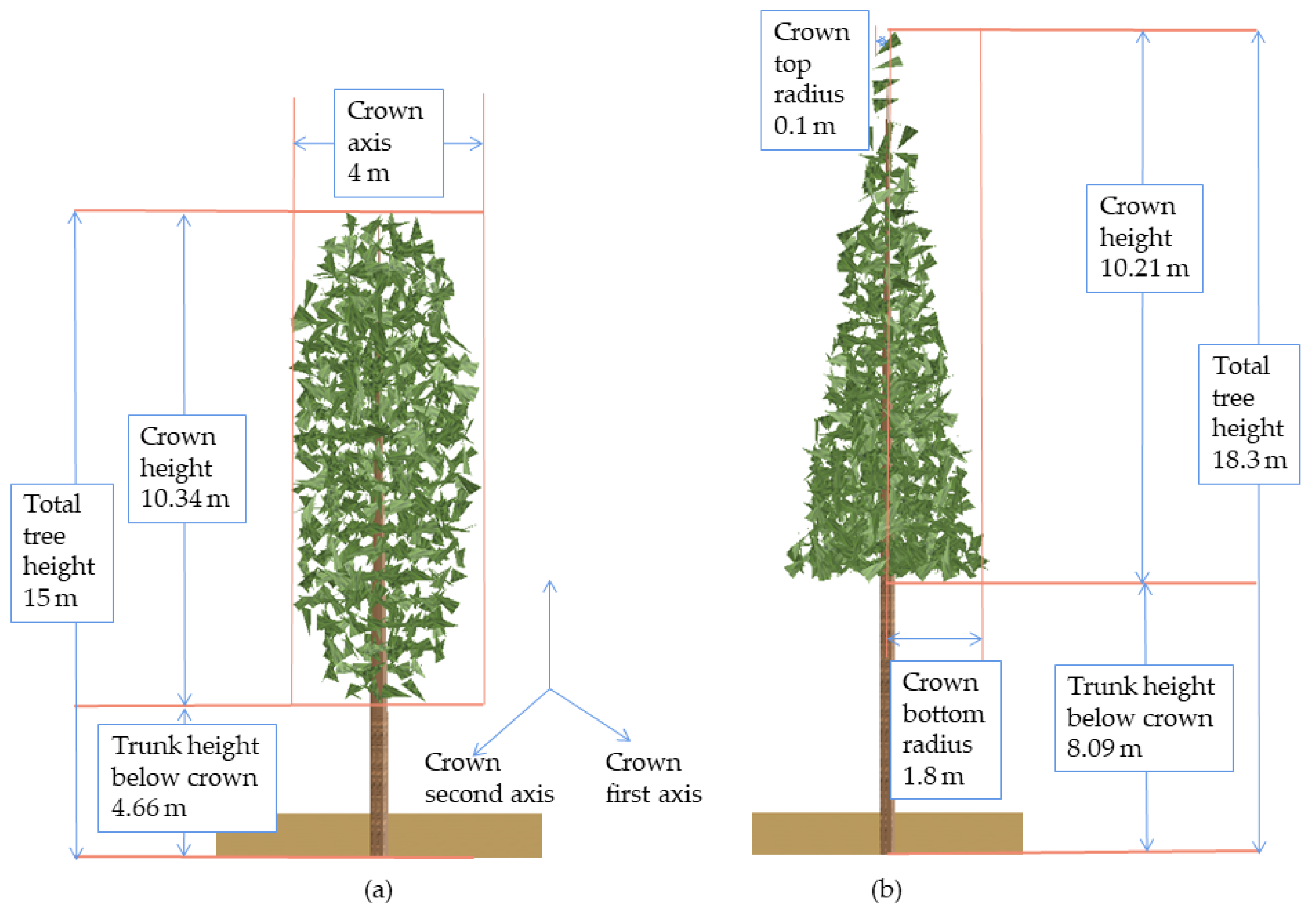
| Tree parameters for broadleaf | Trunk height below crown | [m] | 4.66 |
| Trunk diameter below crown | [m] | 0.36 | |
| Crown type | - | Ellipsoid | |
| Crown height | [m] | 10.34 | |
| Crown first axis | [m] | 4 | |
| Crown second axis | [m] | 4 | |
| Tree parameters for conifer | Trunk height below crown | [m] | 8.09 |
| Trunk diameter below crown | [m] | 0.38 | |
| Crown type | - | Truncated cone | |
| Crown height | [m] | 10.21 | |
| Crown bottom radius | [m] | 1.8 | |
| Crown top radius | [m] | 0.1 |
Publisher’s Note: MDPI stays neutral with regard to jurisdictional claims in published maps and institutional affiliations. |
© 2022 by the authors. Licensee MDPI, Basel, Switzerland. This article is an open access article distributed under the terms and conditions of the Creative Commons Attribution (CC BY) license (https://creativecommons.org/licenses/by/4.0/).
Share and Cite
He, Z.; Lin, S.; Wen, K.; Hao, W.; Chen, L. Effects of Mixture Mode on the Canopy Bidirectional Reflectance of Coniferous–Broadleaved Mixed Plantations. Forests 2022, 13, 235. https://doi.org/10.3390/f13020235
He Z, Lin S, Wen K, Hao W, Chen L. Effects of Mixture Mode on the Canopy Bidirectional Reflectance of Coniferous–Broadleaved Mixed Plantations. Forests. 2022; 13(2):235. https://doi.org/10.3390/f13020235
Chicago/Turabian StyleHe, Zijing, Simei Lin, Kunjian Wen, Wenqian Hao, and Ling Chen. 2022. "Effects of Mixture Mode on the Canopy Bidirectional Reflectance of Coniferous–Broadleaved Mixed Plantations" Forests 13, no. 2: 235. https://doi.org/10.3390/f13020235
APA StyleHe, Z., Lin, S., Wen, K., Hao, W., & Chen, L. (2022). Effects of Mixture Mode on the Canopy Bidirectional Reflectance of Coniferous–Broadleaved Mixed Plantations. Forests, 13(2), 235. https://doi.org/10.3390/f13020235