
Managing Moose from Home: Determining Landscape Carrying Capacity for Alces alces Using Remote Sensing


Abstract
:1. Introduction
2. Materials and Methods
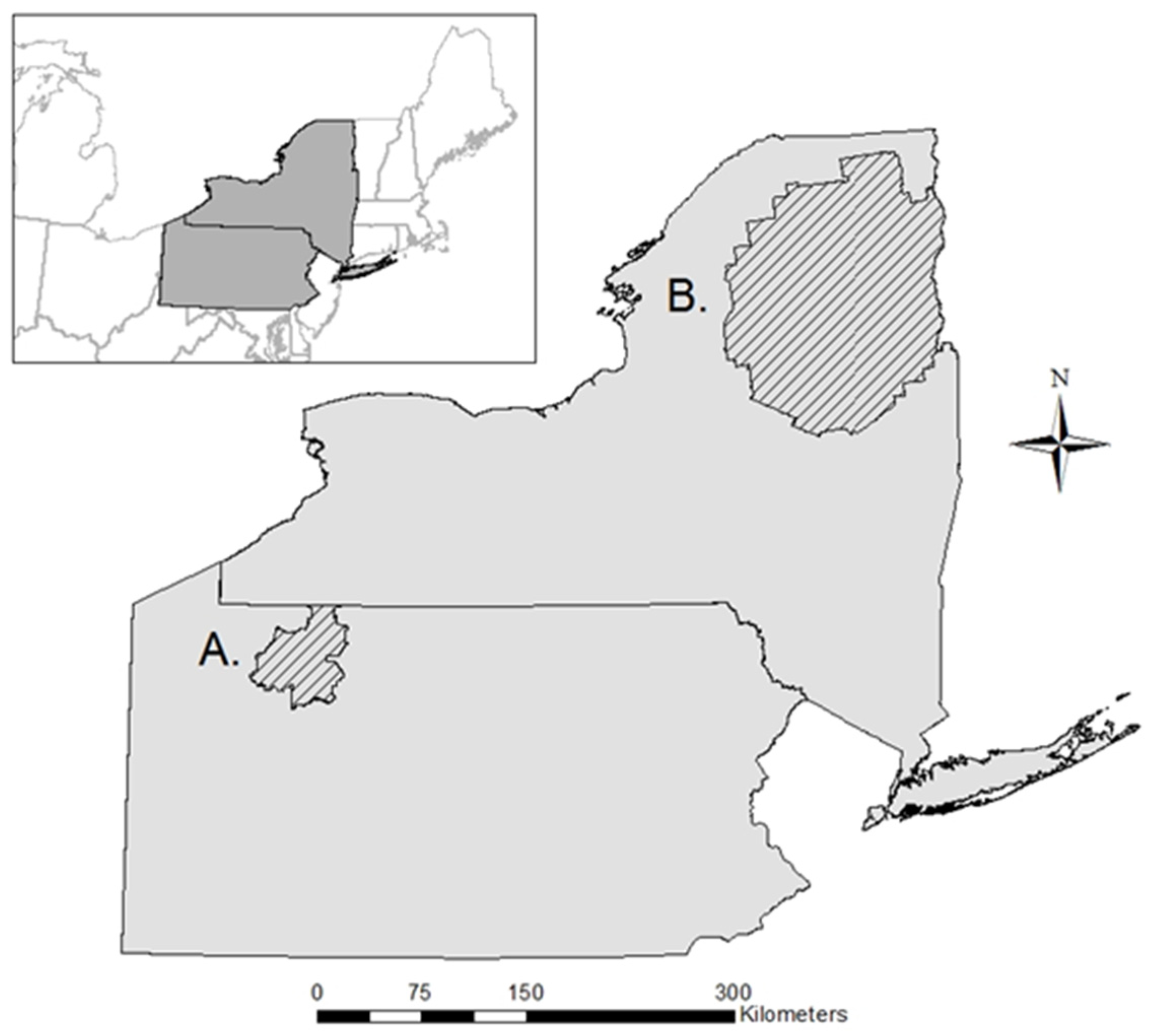
2.1. Study Site
2.1.1. Allegheny National Forest, Northwestern Pennsylvania
2.1.2. Adirondack Park, Northern New York
2.2. Imagery Selection
2.2.1. Allegheny National Forest, Northwestern Pennsylvania
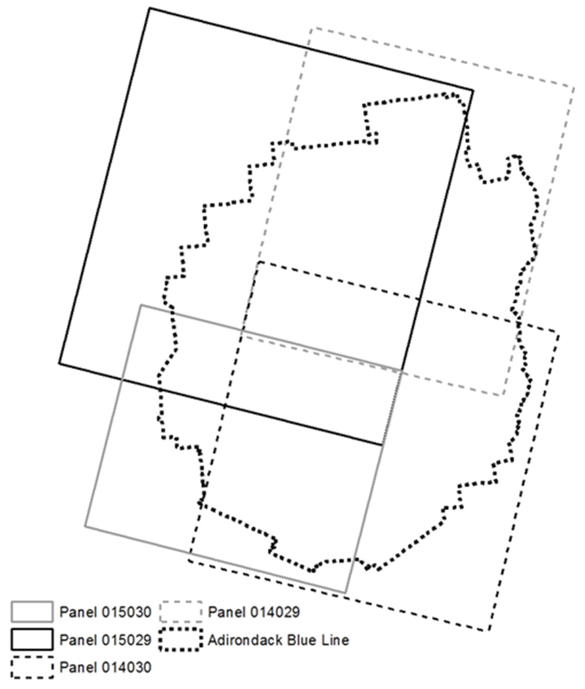
2.2.2. Adirondack Park, Northern New York
2.3. Remote Sensing Classification
2.4. Estimation of Landscape-Level Carrying Capacity for Moose
3. Results
3.1. Allegheny National Forest, Northwestern Pennsylvania
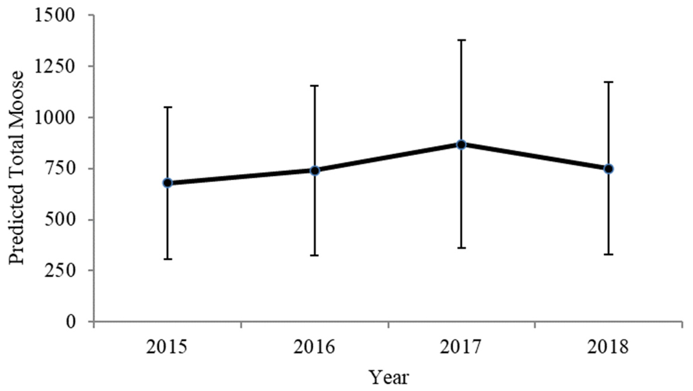
3.2. Adirondack Park, Northern New York
4. Discussion
5. Conclusions
Author Contributions
Funding
Institutional Review Board Statement
Informed Consent Statement
Data Availability Statement
Acknowledgments
Conflicts of Interest
Appendix A
| Panel | Year | Date | Scene |
| Case Study 1: Allegheny National Forest, Pennsylvania | |||
| 017031 | 1991 | 7-Apr | LT50170311991097XXX03 |
| 017031 | 1993 | 30-May | LT50170311993150PAC03 |
| 017031 | 1996 | 26-Aug | LT50170311996239XXX01 |
| 017031 | 2000 | 6-Sep | LT50170312000250XXX03 |
| 017031 | 2002 | 12-Sep | LT50170312002255LGS01 |
| 017031 | 2006 | 9-Oct | LT50170312006282GNC01 |
| 017031 | 2009 | 23-Mar | LT50170312009082GNC01 |
| 017031 | 2013 | 26-Sep | LC80170312013269 |
| Case Study 2: Adirondack Park, New York | |||
| 014029 | 2014 | 8-Sep | LC08_L1TP_014029_20140908_20170303_01_T1 |
| 014029 | 2015 | 27-Sep | LC08_L1TP_014029_20150927_20170225_01_T1 |
| 014029 | 2016 | 13-Sep | LC08_L1TP_014029_20160913_20180130_01_T1 |
| 014029 | 2017 | 30-Jul | LC08_L1TP_014029_20170730_20170811_01_T1 |
| 014029 | 2018 | 5-Oct | LC08_L1TP_014029_20181005_20181010_01_T1 |
| 014030 | 2014 | 6-Jul | LC08_L1TP_014030_20140706_20170304_01_T1 |
| 014030 | 2015 | 27-Sep | LC08_L1TP_014030_20150927_20170225_01_T1 |
| 014030 | 2016 | 13-Sep | LC08_L1TP_014030_20160913_20180130_01_T1 |
| 014030 | 2017 | 30-Jul | LC08_L1TP_014030_20170730_20170811_01_T1 |
| 014030 | 2018 | 5-Oct | LC08_L1TP_014030_20181005_20181010_01_T1 |
| 015029 | 2015 | 16-Jul | LC08_L1TP_015029_20150716_20170226_01_T1 |
| 015029 | 2016 | 4-Sep | LC08_L1TP_015029_20160904_20170221_01_T1 |
| 015029 | 2017 | 23-Sep | LC08_L1TP_015029_20170923_20171013_01_T1 |
| 015029 | 2018 | 22-Jun | LC08_L1TP_015029_20180622_20180703_01_T1 |
| 015030 | 2013 | 28-Sep | LC08_L1TP_015030_20130928_20170308_01_T1 |
| 015030 | 2015 | 16-Jul | LC08_L1TP_015030_20150716_20170226_01_T1 |
| 015030 | 2016 | 20-Sep | LC08_L1TP_015030_20160920_20170221_01_T1 |
| 015030 | 2017 | 23-Sep | LC08_L1TP_015030_20170923_20171013_01_T1 |
| 015030 | 2018 | 21-May | LC08_L1TP_015030_20180521_20180605_01_T1 |
Appendix B
| A. | Pennsylvania | ||||
| Reference | |||||
| 1993 | Mature | Overstory Removal | Intermediate Removal | User’s Accuracy | |
| Classification | Mature | 107 | 0 | 0 | 1.00 |
| Overstory Removal | 0 | 113 | 8 | 0.93 | |
| Intermediate Removal | 3 | 0 | 19 | 0.86 | |
| Producer’s Accuracy | 0.97 | 1.00 | 0.71 | ||
| Overall Accuracy (%) | 95.5 | ||||
| Kappa Index | 0.92 | ||||
| Reference | |||||
| 1996 | Mature | Overstory Removal | Intermediate Removal | User’s Accuracy | |
| Classification | Mature | 100 | 0 | 0 | 1.00 |
| Overstory Removal | 0 | 113 | 8 | 0.93 | |
| Intermediate Removal | 5 | 3 | 20 | 0.71 | |
| Producer’s Accuracy | 0.95 | 0.97 | 0.71 | ||
| Overall Accuracy (%) | 93.3 | ||||
| Kappa Index | 0.89 | ||||
| Reference | |||||
| 2000 | Mature | Overstory Removal | Intermediate Removal | User’s Accuracy | |
| Classification | Mature | 98 | 0 | 0 | 1.00 |
| Overstory Removal | 0 | 99 | 5 | 0.95 | |
| Intermediate Removal | 2 | 0 | 46 | 0.97 | |
| Producer’s Accuracy | 0.98 | 1.00 | 0.91 | ||
| Overall Accuracy (%) | 97.4 | ||||
| Kappa Index | 0.96 | ||||
| Reference | |||||
| 2002 | Mature | Overstory Removal | Intermediate Removal | User’s Accuracy | |
| Classification | Mature | 89 | 0 | 0 | 1.00 |
| Overstory Removal | 2 | 89 | 14 | 0.85 | |
| Intermediate Removal | 0 | 0 | 57 | 1.00 | |
| Producer’s Accuracy | 0.98 | 1.00 | 0.80 | ||
| Overall Accuracy (%) | 93.7 | ||||
| Kappa Index | 0.9 | ||||
| Reference | |||||
| 2006 | Mature | Overstory Removal | Intermediate Removal | User’s Accuracy | |
| Classification | Mature | 94 | 0 | 0 | 1.00 |
| Overstory Removal | 0 | 83 | 2 | 0.98 | |
| Intermediate Removal | 8 | 4 | 59 | 0.83 | |
| Producer’s Accuracy | 0.92 | 0.95 | 0.97 | ||
| Overall Accuracy (%) | 94.5 | ||||
| Kappa Index | 0.92 | ||||
| Reference | |||||
| 2009 | Mature | Overstory Removal | Intermediate Removal | User’s Accuracy | |
| Classification | Mature | 121 | 0 | 1 | 0.99 |
| Overstory Removal | 1 | 49 | 15 | 0.75 | |
| Intermediate Removal | 3 | 1 | 58 | 0.93 | |
| Producer’s Accuracy | 0.97 | 0.97 | 0.78 | ||
| Overall Accuracy (%) | 91.2 | ||||
| Kappa Index | 0.86 | ||||
| Reference | |||||
| 2013 | Mature | Overstory Removal | Intermediate Removal | User’s Accuracy | |
| Classification | Mature | 109 | 0 | 0 | 1.00 |
| Overstory Removal | 0 | 56 | 13 | 0.81 | |
| Intermediate Removal | 1 | 3 | 68 | 0.94 | |
| Producer’s Accuracy | 0.99 | 0.95 | 0.84 | ||
| Overall Accuracy (%) | 93.1 | ||||
| Kappa Index | 0.89 | ||||
| B. | New York | ||||
| Reference | |||||
| Panel 014029—2014 | Mature | Overstory Removal | Intermediate Removal | User’s Accuracy | |
| Classification | Mature | 267 | 2 | 13 | 0.95 |
| Overstory Removal | 23 | 4 | 138 | 0.84 | |
| Intermediate Removal | 12 | 142 | 51 | 0.69 | |
| Producer’s Accuracy | 0.88 | 0.96 | 0.68 | ||
| Overall Accuracy (%) | 83.9 | ||||
| Kappa Index | 0.75 | ||||
| Reference | |||||
| Panel 014029—2015 | Mature | Overstory Removal | Intermediate Removal | User’s Accuracy | |
| Classification | Mature | 322 | 0 | 13 | 0.96 |
| Overstory Removal | 48 | 4 | 422 | 0.89 | |
| Intermediate Removal | 0 | 57 | 38 | 0.6 | |
| Producer’s Accuracy | 0.87 | 0.93 | 0.89 | ||
| Overall Accuracy (%) | 88.6 | ||||
| Kappa Index | 0.8 | ||||
| Reference | |||||
| Panel 014029—2016 | Mature | Overstory Removal | Intermediate Removal | User’s Accuracy | |
| Classification | Mature | 312 | 0 | 23 | 0.93 |
| Overstory Removal | 36 | 3 | 435 | 0.92 | |
| Intermediate Removal | 0 | 60 | 35 | 0.63 | |
| Producer’s Accuracy | 0.9 | 0.95 | 0.88 | ||
| Overall Accuracy (%) | 89.3 | ||||
| Kappa Index | 0.81 | ||||
| Reference | |||||
| Panel 014029—2017 | Mature | Overstory Removal | Intermediate Removal | User’s Accuracy | |
| Classification | Mature | 301 | 3 | 31 | 0.9 |
| Overstory Removal | 30 | 6 | 438 | 0.92 | |
| Intermediate Removal | 0 | 65 | 30 | 0.68 | |
| Producer’s Accuracy | 0.91 | 0.88 | 0.88 | ||
| Overall Accuracy (%) | 88.9 | ||||
| Kappa Index | 0.80 | ||||
| Reference | |||||
| Panel 014029—2018 | Mature | Overstory Removal | Intermediate Removal | User’s Accuracy | |
| Classification | Mature | 336 | 3 | 26 | 0.92 |
| Overstory Removal | 34 | 3 | 397 | 0.91 | |
| Intermediate Removal | 5 | 73 | 27 | 0.7 | |
| Producer’s Accuracy | 0.9 | 0.92 | 0.88 | ||
| Overall Accuracy (%) | 89.2 | ||||
| Kappa Index | 0.81 | ||||
| Reference | |||||
| Panel 014030—2014 | Mature | Overstory Removal | Intermediate Removal | User’s Accuracy | |
| Classification | Mature | 335 | 0 | 22 | 0.94 |
| Overstory Removal | 52 | 4 | 625 | 0.92 | |
| Intermediate Removal | 0 | 105 | 70 | 0.6 | |
| Producer’s Accuracy | 0.87 | 0.96 | 0.87 | ||
| Overall Accuracy (%) | 87.8 | ||||
| Kappa Index | 0.78 | ||||
| Reference | |||||
| Panel 014030—2015 | Mature | Overstory Removal | Intermediate Removal | User’s Accuracy | |
| Classification | Mature | 554 | 0 | 32 | 0.82 |
| Overstory Removal | 77 | 5 | 363 | 0.95 | |
| Intermediate Removal | 0 | 74 | 75 | 0.5 | |
| Producer’s Accuracy | 0.77 | 0.94 | 0.88 | ||
| Overall Accuracy (%) | 84.0 | ||||
| Kappa Index | 0.72 | ||||
| Reference | |||||
| Panel 014030—2016 | Mature | Overstory Removal | Intermediate Removal | User’s Accuracy | |
| Classification | Mature | 597 | 0 | 33 | 0.95 |
| Overstory Removal | 83 | 3 | 336 | 0.8 | |
| Intermediate Removal | 0 | 51 | 77 | 0.4 | |
| Producer’s Accuracy | 0.88 | 0.94 | 0.75 | ||
| Overall Accuracy (%) | 83.4 | ||||
| Kappa Index | 0.70 | ||||
| Reference | |||||
| Panel 014030—2017 | Mature | Overstory Removal | Intermediate Removal | User’s Accuracy | |
| Classification | Mature | 586 | 0 | 44 | 0.93 |
| Overstory Removal | 79 | 2 | 341 | 0.81 | |
| Intermediate Removal | 0 | 49 | 79 | 0.38 | |
| Producer’s Accuracy | 0.88 | 0.96 | 0.73 | ||
| Overall Accuracy (%) | 82.7 | ||||
| Kappa Index | 0.69 | ||||
| Reference | |||||
| Panel 014030—2018 | Mature | Overstory Removal | Intermediate Removal | User’s Accuracy | |
| Classification | Mature | 926 | 2 | 12 | 0.99 |
| Overstory Removal | 73 | 17 | 57 | 0.39 | |
| Intermediate Removal | 5 | 62 | 26 | 0.67 | |
| Producer’s Accuracy | 0.92 | 0.77 | 0.6 | ||
| Overall Accuracy (%) | 88.6 | ||||
| Kappa Index | 0.63 | ||||
| Reference | |||||
| Panel 015029—2015 | Mature | Overstory Removal | Intermediate Removal | User’s Accuracy | |
| Classification | Mature | 684 | 0 | 37 | 0.95 |
| Overstory Removal | 63 | 14 | 467 | 0.86 | |
| Intermediate Removal | 1 | 216 | 74 | 0.74 | |
| Producer’s Accuracy | 0.91 | 0.96 | 0.81 | ||
| Overall Accuracy (%) | 87.9 | ||||
| Kappa Index | 0.80 | ||||
| Reference | |||||
| Panel 015029—2016 | Mature | Overstory Removal | Intermediate Removal | User’s Accuracy | |
| Classification | Mature | 680 | 0 | 41 | 0.94 |
| Overstory Removal | 49 | 13 | 482 | 0.89 | |
| Intermediate Removal | 1 | 216 | 74 | 0.74 | |
| Producer’s Accuracy | 0.93 | 0.94 | 0.81 | ||
| Overall Accuracy (%) | 88.6 | ||||
| Kappa Index | 0.82 | ||||
| Reference | |||||
| Panel 015029—2017 | Mature | Overstory Removal | Intermediate Removal | User’s Accuracy | |
| Classification | Mature | 754 | 0 | 47 | 0.94 |
| Overstory Removal | 61 | 26 | 379 | 0.81 | |
| Intermediate Removal | 5 | 208 | 76 | 0.72 | |
| Producer’s Accuracy | 0.92 | 0.89 | 0.75 | ||
| Overall Accuracy (%) | 86.2 | ||||
| Kappa Index | 0.77 | ||||
| Reference | |||||
| Panel 015029—2018 | Mature | Overstory Removal | Intermediate Removal | User’s Accuracy | |
| Classification | Mature | 896 | 4 | 52 | 0.94 |
| Overstory Removal | 68 | 23 | 252 | 0.73 | |
| Intermediate Removal | 15 | 190 | 56 | 0.73 | |
| Producer’s Accuracy | 0.92 | 0.88 | 0.7 | ||
| Overall Accuracy (%) | 86.0 | ||||
| Kappa Index | 0.74 | ||||
| Reference | |||||
| Panel 015030—2013 | Mature | Overstory Removal | Intermediate Removal | User’s Accuracy | |
| Classification | Mature | 111 | 0 | 27 | 0.8 |
| Overstory Removal | 19 | 4 | 192 | 0.89 | |
| Intermediate Removal | 0 | 14 | 51 | 0.25 | |
| Producer’s Accuracy | 0.85 | 0.78 | 0.74 | ||
| Overall Accuracy (%) | 75.8 | ||||
| Kappa Index | 0.57 | ||||
| Reference | |||||
| Panel 015030—2015 | Mature | Overstory Removal | Intermediate Removal | User’s Accuracy | |
| Classification | Mature | 153 | 0 | 18 | 0.89 |
| Overstory Removal | 12 | 2 | 265 | 0.95 | |
| Intermediate Removal | 0 | 29 | 11 | 0.72 | |
| Producer’s Accuracy | 0.93 | 0.94 | 0.9 | ||
| Overall Accuracy (%) | 91.2 | ||||
| Kappa Index | 0.84 | ||||
| Reference | |||||
| Panel 015030—2016 | Mature | Overstory Removal | Intermediate Removal | User’s Accuracy | |
| Classification | Mature | 244 | 0 | 13 | 0.95 |
| Overstory Removal | 20 | 4 | 169 | 0.88 | |
| Intermediate Removal | 0 | 29 | 11 | 0.72 | |
| Producer’s Accuracy | 0.92 | 0.88 | 0.88 | ||
| Overall Accuracy (%) | 90.2 | ||||
| Kappa Index | 0.82 | ||||
| Reference | |||||
| Panel 015030—2017 | Mature | Overstory Removal | Intermediate Removal | User’s Accuracy | |
| Classification | Mature | 215 | 0 | 16 | 0.93 |
| Overstory Removal | 12 | 4 | 195 | 0.92 | |
| Intermediate Removal | 0 | 34 | 14 | 0.71 | |
| Producer’s Accuracy | 0.95 | 0.89 | 0.87 | ||
| Overall Accuracy (%) | 90.6 | ||||
| Kappa Index | 0.84 | ||||
| Reference | |||||
| Panel 015030—2018 | Mature | Overstory Removal | Intermediate Removal | User’s Accuracy | |
| Classification | Mature | 238 | 0 | 13 | 0.95 |
| Overstory Removal | 23 | 8 | 141 | 0.82 | |
| Intermediate Removal | 1 | 50 | 16 | 0.75 | |
| Producer’s Accuracy | 0.91 | 0.86 | 0.83 | ||
| Overall Accuracy (%) | 87.6 | ||||
| Kappa Index | 0.79 | ||||
References
- De Calesta, D.S.; Stout, S.L. Relative deer density and sustainability: A conceptual framework for integrating deer management with ecosystem management. Wildl. Soc. Bull. 1997, 25, 252–285. [Google Scholar]
- McCullough, D.R. The George Reserve Deer Herd: Population Ecology of a K-Selected Species; University of Michigan Press: Ann Arbor, MI, USA, 1979; p. 271. [Google Scholar]
- Macnab, J. Carrying capacity and related slippery shibboleths. Wildl. Soc. Bull. 1985, 13, 403–410. [Google Scholar]
- Hobbs, N.T.; Swift, D.M. Estimates of habitat carrying capacity incorporating explicit nutritional constraints. J. Wildl. Manag. 1985, 49, 814–822. [Google Scholar] [CrossRef]
- Crête, M. Approximation of K carrying capacity for moose in eastern Quebec. Can. J. Zool. 1989, 67, 373–380. [Google Scholar] [CrossRef]
- Wam, K.H.; Hjeljord, O.; Soldberg, E.J. Differential forage use makes carrying capacity equivocal on ranges of Scandanavian moose (Alces alces). Can. J. Zool. 2010, 88, 1179–1191. [Google Scholar] [CrossRef]
- Razenkova, E.; Radeloff, V.; Dubinin, M.; Bragina, E.; Allen, A.; Clayton, M.; Pidgeon, A.; Baskin, L.; Coops, N.; Hobi, M. Vegetation productivity summarized by the Dynamic Habitat Indices explains broad-scale patterns of moose abundance across Russia. Sci. Rep. 2020, 10, 836. [Google Scholar] [CrossRef] [PubMed] [Green Version]
- Doan, T.; Guo, X. Understanding bison carrying capacity estimation in Northern Great Plains using remote sensing and GIS. Can. J. Remote Sens. 2019, 45, 139–162. [Google Scholar] [CrossRef]
- O’Hara, L.O.; Latham, P.A.; Hessburg, P.; Smith, B.G. A structural classification for inland Northwest forest vegetation. West. J. Appl. For. 1996, 11, 97–102. [Google Scholar] [CrossRef] [Green Version]
- Brockerhoff, E.G.; Barbaro, L.; Castagneyrol, B.; Forrester, D.; Gardiner, B.; González-Olabarria, J.; Lyver, P.; Meurisse, N.; Oxbrough, A.; Taki, H.; et al. Forest biodiversity, ecosystem functioning and the provision of ecosystem services. Biodivers. Conserv. 2017, 26, 3005–3035. [Google Scholar] [CrossRef] [Green Version]
- Hummel, S.; Hudak, A.; Uebler, E.; Falkowski, M.; Megown, K. A comparison of accuracy and cost of LiDAR versus stand exam data for landscape management on the Malhuer National Forest. J. For. 2011, 109, 267–273. [Google Scholar]
- Beland, M.; Parker, G.; Sparrow, B.; Harding, D.; Chasmer, L.; Phinn, S.; Antonarakis, A.; Strahler, A. On promoting the use of LiDAR systems in forest ecosystem research. For. Ecol. Manag. 2019, 450, 117484. [Google Scholar] [CrossRef]
- LaRue, E.A.; Wagner, F.; Fei, S.; Atkins, J.; Fahey, R.; Gough, C.; Hardiman, B.B. Compatibility of aerial and terrestrial LiDAR for quantifying forest structural diversity. Remote Sens. 2020, 12, 1407. [Google Scholar] [CrossRef]
- Coops, N.C.; Hilker, T.; Wulder, M.A.; St-Onge, B.; Newnham, G.; Siggins, A.; Trofymow. J.A. Estimating canopy structure of Douglas-fir forests from discrete-return LiDAR. Trees 2007, 21, 295–310. [Google Scholar] [CrossRef] [Green Version]
- Clark, D.B.; Olivas, P.C.; Oberbauer, S.F.; Clark, D.A.; Ryan, M.G. First direct landscape-scale measurement of tropical rain forest leaf area index, a key driver of global primary productivity. Ecol. Lett. 2008, 11, 163–172. [Google Scholar] [CrossRef]
- Falkowski, M.J.; Evans, J.S.; Martinuzzi, S.; Gessler, P.E.; Hudak, A.T. Characterizing forest succession with LIDAR data: An evaluation for Inland Northwest, USA. Remote Sens. Environ. 2009, 113, 946–956. [Google Scholar] [CrossRef] [Green Version]
- Bergen, K.M.; Dronova, I. Observing succession on aspen-dominated landscape using remote sensing-ecosystem approach. Landsc. Ecol. 2007, 22, 1395–1410. [Google Scholar] [CrossRef]
- Hao, Z.; Xhang, J.; Song, B.; Ye, J.; Li, B. Vertical structure and spatial associations of dominant tree species in an old-growth temperature forest. For. Ecol. Manag. 2007, 252, 1–11. [Google Scholar] [CrossRef]
- Baker, W.L. A review of models of landscape change. Landsc. Ecol. 1989, 1, 111–133. [Google Scholar] [CrossRef]
- Shugart, H.H. The importance of structure in the longer-term dynamics of ecosystems. J. Geophys. Res–Atmos. 2000, 105, 20065–20075. [Google Scholar] [CrossRef]
- Homer, C.G.; Dewitz, J.; Yang, L.; Jin, S.; Danielson, P.; Xian, G.; Coulston, J.; Herold, N.; Wickham, J.; Megown, K. Completion of the 2011 National Land Cover Database for the conterminous United States-Representing a decade of land cover change information. Photogramm. Eng. Remote Sens. 2015, 81, 345–354. [Google Scholar]
- Madden, M. (Ed.) Manual of Geographic Information Systems; American Society for Photogrammetry and Remote Sensing: Bethesda, MD USA, 2009; p. 1330. [Google Scholar]
- Peters, A.J.; Walter-Shea, E.A.; Ji, L.; Vina, A.; Hayes, M.; Svoboda, M.D. Drought monitoring with NDVI-based standardized vegetation index. Photogramm. Eng. Remove Sens. 2002, 68, 71–75. [Google Scholar]
- Gu, Y.; Brown, J.F.; Verdin, J.P.; Wardlow, B. A five-year analysis of MODIS NDVI and NDWI for grassland drought assessment over the central Great Plains of the United States. Geophys. Res. Lett. 2007, 34, 6. [Google Scholar] [CrossRef] [Green Version]
- Hebblewhite, M.; Merrill, E.; McDermid, G. A multi-scale test of the forage maturation hypothesis in a partially migratory ungulate population. Ecol. Monogr. 2008, 78, 141–166. [Google Scholar] [CrossRef] [Green Version]
- Hansen, B.B.; Aanes, R.; Herfindal, I.; Saether, B.; Henriksen, S. Winter habitat–space use in a large arctic herbivore facing contrasting forage abundance. Polar Biol. 2009, 32, 971–984. [Google Scholar] [CrossRef]
- Quarmby, N.A.; Milnes, M.; Hindle, T.L.; Silleos, N. The use of multi-temporal NDVI measurements from AVHRR data for crop yield estimation and prediction. Int. J. Remote Sens. 1993, 14, 199–210. [Google Scholar] [CrossRef]
- Hayes, M.J.; Decker, W.L. Using NOAA AVHRR data to estimate maize production in the United States Corn Belt. Int. J. Remote Sens. 1996, 17, 3189–3200. [Google Scholar] [CrossRef]
- Wilson, E.H.; Sader, S.A. Detection of forest harvest type using multiple dates of Landsat TM imagery. Remote Sens. Environ. 2002, 80, 385–396. [Google Scholar] [CrossRef]
- Renecker, L.A.; Hudson, R.J. Seasonal energy expenditures and thermoregulatory responses of moose. Can. J. Zool. 1986, 64, 322–327. [Google Scholar] [CrossRef]
- Fisher, J.T.; Wilkinson, L. The response of mammals to forest fire and timber harvest in the North America boreal forest. Mammal Rev. 2005, 35, 51–81. [Google Scholar] [CrossRef]
- Schrempp, T.V.; Rachlow, J.; Johnson, R.; Shipley, L.; Long, R.; Aycrigg, J.; Hurley, M. Linking forest management to moose population trends: The role of the nutritional landscape. PLoS ONE 2019, 14, e0219128. [Google Scholar] [CrossRef] [Green Version]
- Peterson, S.; Kramer, D.; Hurst, J.; Frair, J. Browse selection by moose in the Adirondack Park, New York. Alces 2020, 56, 107–126. [Google Scholar]
- Regelin, W.L.; Schwartz, C.; Franzmann, A. Effects of forest succession on nutritional dynamics of moose forage. Swed. Wildl. Res. Suppl. 1987, 1, 247–264. [Google Scholar]
- Saether, B.E.; Andersen, R. Resource limitation in a generalist herbivore, the moose, (Alces alces): Ecological constraints on behavioral decisions. Can. J. Zool. 1990, 68, 993–999. [Google Scholar] [CrossRef]
- Milligan, H.R.; Koricheva, J. Effects of tree species richness and composition on moose winter browsing damage and foraging selectivity: An experimental study. J. Anim. Ecol. 2013, 82, 739–748. [Google Scholar] [CrossRef]
- Mumma, M.A.; Gillingham, M.; Marshall, S.; Proctor, C.; Bevington, A.; Scheideman, M. Regional moose (Alces alces) responses to forestry cutblocks are driven by landscape-scale patterns of vegetation composition and regrowth. For. Ecol. Manag. 2021, 481, 118763. [Google Scholar] [CrossRef]
- Thompson, I.D.; Stewart, R.W. Management of Moose Habitat. In Ecology and Management of the North American Moose, 2nd ed.; Schwartz, C., Franzmann, A., McCabe, R., Eds.; Smithsonian Institution Press: Washington, DC, USA, 1997; pp. 377–401. [Google Scholar]
- Peterson, S. Browse Selection and Constraints for Moose (Alces alces) in the Adirondack Park, New York, USA. Master’s Thesis, State University of New York, College of Environmental Science and Forestry, Syracuse, New York, NY, USA, 2018. [Google Scholar]
- Hough, A.; Forbes, R. The ecology and silvics of forests in the high plateau of Pennsylvania. Ecol. Monogr. 1943, 13, 299–320. [Google Scholar] [CrossRef]
- Anacker, B.L.; Kirschbaum, C.D. Vascular flora of the Kinzua Quality Deer Cooperative, northwestern Pennsylvania, U.S.A. Bartonia 2006, 63, 11–28. [Google Scholar]
- Redding, J. History of Deer Population Trends and Forest Cutting on the Allegheny National Forest; General Technical Report NE-197; U.S. Department of Agriculture, Forest Service, Northeastern Forest Experiment Station: Warren, PA, USA, 1995.
- Bjorkbom, J.C.; Larson, R.G. The Tionesta Scenic and Research Natural Areas; General Technical Report NE-31; USDA Forest Service, Northeastern Forest Experiment Station: Warren, PA, USA, 1977.
- Menne, M.J.; Williams, C.N.; Vose, R.S. The United States historical climatology network monthly temperature data-version 2. Bull. Am. Meteorol. Soc. 2009, 90, 993–1107. [Google Scholar] [CrossRef] [Green Version]
- Lumber Heritage Region of Pennsylvania. Management Action Plan, May 2001; Lumber Heritage Region: Emporium, PA, USA, 2001; p. 86. [Google Scholar]
- Nyland, R.D. Silviculture: Concepts and Applications; McGraw-Hill Higher Education: Burr Ridge, IL, USA, 2002. [Google Scholar]
- Marquis, D.; Ernst, R.; Stout, S. Prescribing Silvicultural Treatments in Hardwood Stands of the Alleghenies (Revised); General Technical Report NE-96; USDA Forest Service, Northeastern Forest Experiment Station: Radnor, PA, USA, 1992.
- Jenkins, J.; Keal, A. The Adirondack Atlas: A Geographic Portrait of the Adirondack Park; Syracuse University Press: Syracuse, NY, USA, 2004. [Google Scholar]
- Breiman, L. Random forests. Mach. Learn. 2001, 45, 5–32. [Google Scholar] [CrossRef] [Green Version]
- Liaw, A.; Wiener, M. Classification and regression by Random Forest. R News 2002, 2, 18–22. [Google Scholar]
- Shanley, C.S.; Eacker, D.; Reynolds, C.; Bennetsen, B.; Gilbert, S. Using LiDAR and Random Forest to improve deer habitat models in a managed forest landscape. For. Ecol. Manag. 2021, 499, 119580. [Google Scholar] [CrossRef]
- Chavez, P.S., Jr.; MacKinnon, D.J. Automatic detection of vegetation changes in the Southwestern United States using remotely sensed images. Photogramm. Eng. Remote Sens. 1994, 60, 571–583. [Google Scholar]
- Eidenshink, J.C.; Faudeen, J.L. The 1-km AVHRR global land data set: First stages in implementation. Int. J. Remote Sens. 1994, 15, 3443–3462. [Google Scholar] [CrossRef]
- Drake, N.A.; Mackin, S.; Settle, J.J. Mapping vegetation, soils, and geology in semiarid shrublands using spectral matching and mixture modeling of SWIR AVIRIS imagery. Remove Sens. Environ. 1999, 68, 12–25. [Google Scholar] [CrossRef]
- Lewis, H.G.; Brown, M. A generalized confusion matrix for assessing area estimate from remotely sensed data. Int. J. Remote Sens. 2001, 22, 3223–3235. [Google Scholar] [CrossRef]
- Landis, J.R.; Koch, G. An application of hierarchical kappa-type statistics in the assessment of majority agreement among multiple observers. Biometrics 1977, 33, 363–374. [Google Scholar] [CrossRef] [PubMed]
- Homer, C.G.; Dewitz, J.; Jin, S.; Xian, G.; Costello, C.; Danielson, P.; Gass, L.; Funk, M.; Wickham, J.; Stehman, S.; et al. Conterminous United States land cover change patterns 2001–2016 from the 2016 National Land Cover Database. ISPRS J. Photogramm. Remote Sens. 2020, 162, 184–199. [Google Scholar] [CrossRef]
- Adirondack Park Agency. Wetlands Effects Database and GIS for the Adirondack Park. 2004. Available online: https://apa.ny.gov/Research/ParkwideGISFinalReport.pdf (accessed on 5 January 2018).
- Renecker, L.A.; Schwartz, C.C. Food Habits and Feeding Behavior. In Ecology and Management of the North American Moose, 2nd ed.; Schwartz, C., Franzmann, A., McCabe, R., Eds.; Smithsonian Institution Press: Washington, DC, USA, 1997; pp. 403–440. [Google Scholar]
- Hinton, J.H.; Wheat, R.E.; Schuette, P.; Hurst, J.; Kramer, D.; Frair, J. Challenges and opportunities for robust population monitoring of moose along their southern range in eastern North America. J. Wildl. Manag. Accepted.
- Hanberry, B.B. Addressing regional relationships between white-tailed deer densities and land classes. Ecol. Evol. 2021, 11, 13570–13578. [Google Scholar] [CrossRef]
- Hill, R.A.; Thomson, A.G. Mapping woodland species composition and structure using airborne spectral and LiDAR data. Int. J. Remote Sens. 2005, 26, 3763–3779. [Google Scholar] [CrossRef]
- Blouin, J.; DeBow, J.; Rosenblatt, E.; Hines, J.; Alexander, C.; Gieder, K.; Fortin, N.; Murdoch, J.; Donovan, T. Moose habitat selection and fitness consequences during two critical winter tick life stages in Vermont, United States. Front. Ecol. Evol. 2021, 9, 642276. [Google Scholar] [CrossRef]
- Peek, J.M. Habitat Relationships. In Ecology and Management of the North American Moose, 2nd ed.; Schwartz, C., Franzmann, A., McCabe, R., Eds.; Smithsonian Institution Press: Washington, DC, USA, 1997; pp. 351–376. [Google Scholar]
- Stewart, K.M.; Bowyer, R.T.; Wiesburg, P.J. Biology and Management of White-Tailed Deer, 1st ed.; CRC Press: Boca Raton, FL, USA, 2011; pp. 181–218. [Google Scholar]


| Predictors |
|---|
| NDVI (target scene year) |
| NDVI (previous scene year) |
| Difference NDVI (previous target) |
| Difference in 1.55–1.75 mm Band (previous target) |
| Difference in 2.09–2.35 mm Band (previous target) |
| Previous panel prediction (e.g., 2015 landscape for 2016 target scene) |
| NLCD Class | Reclassified |
|---|---|
| Open water | Water |
| Developed, open space | Developed |
| Developed, low intensity | Developed |
| Developed, medium intensity | Developed |
| Developed, high intensity | Developed |
| Rock/clay/sand | Developed |
| Deciduous forest | Mature Forest |
| Evergreen forest | Conifer |
| Mixed forest | Mature Forest |
| Scrubland | Grass/Scrub |
| Grassland | Grass/Scrub |
| Pasture/hay | Agriculture |
| Cultivated crops | Agriculture |
| Woody wetlands | Wetlands |
| Herbaceous wetlands | Grass |
| Land Cover Type | Moose/km2 |
|---|---|
| Conifer forest | 0 |
| Upland deciduous forest/mixed forest | 0.0028 |
| Lowland deciduous forest/mixed forest | 0 |
| Wooded wetland | 0 |
| Open wetland | 0 |
| Regenerating forest | 0.0195 |
| A. Study 1: Allegheny National Forest, PA | ||
| Year | Overall Accuracy (%) | Cohen’s Kappa |
| 1993 | 95.5 | 0.92 |
| 1996 | 93.3 | 0.89 |
| 2000 | 97.4 | 0.96 |
| 2002 | 93.7 | 0.9 |
| 2006 | 94.5 | 0.92 |
| 2009 | 91.2 | 0.86 |
| 2013 | 93.1 | 0.89 |
| B. Study 2: Adirondack Park, New York | ||
| Year | Overall Accuracy (%) | Cohen’s Kappa |
| Panel 014029 | ||
| 2104 | 83.9 | 0.75 |
| 2015 | 88.6 | 0.8 |
| 2016 | 89.3 | 0.81 |
| 2017 | 88.9 | 0.8 |
| 2018 | 89.2 | 0.81 |
| Panel 014030 | ||
| 2104 | 87.8 | 0.78 |
| 2015 | 84 | 0.72 |
| 2016 | 83.4 | 0.7 |
| 2017 | 82.7 | 0.69 |
| 2018 | 88.6 | 0.63 |
| Panel 015029 | ||
| 2015 | 87.9 | 0.8 |
| 2016 | 88.6 | 0.82 |
| 2017 | 86.2 | 0.77 |
| 2018 | 86 | 0.74 |
| Panel 015030 | ||
| 2013 | 75.8 | 0.57 |
| 2015 | 91.2 | 0.84 |
| 2016 | 90.2 | 0.82 |
| 2017 | 90.6 | 0.84 |
| 2018 | 87.6 | 0.79 |
| Land Cover Class | Year | ||||||||
|---|---|---|---|---|---|---|---|---|---|
| Allegheny National Forest | 1993 | 1996 | 2000 | 2002 | 2006 | 2009 | 2013 | AVG. | STDEV |
| Mature Forest | 75.52 | 79.24 | 71.56 | 72.72 | 57.06 | 68.15 | 63.28 | 69.65 | 7.54 |
| Overstory Removal | 1.1 | 2.0 | 1.0 | 0.8 | 13.2 | 1.0 | 1.1 | 2.9 | 4.6 |
| Intermediate Removal | 7.3 | 2.7 | 3.8 | 2.8 | 6.7 | 7.8 | 12.2 | 6.2 | 3.4 |
| Conifer | 7.3 | 7.3 | 6.1 | 6.1 | 6.0 | 6.5 | 6.0 | 6.4 | 0.6 |
| Grass/Scrubland | 0.5 | 0.5 | 7.0 | 7.0 | 6.6 | 6.1 | 7.1 | 5.0 | 3.1 |
| Water | 0.6 | 0.6 | 0.8 | 0.8 | 0.8 | 0.8 | 0.7 | 0.7 | 0.1 |
| Developed | 1.0 | 1.0 | 3.2 | 3.2 | 3.2 | 3.2 | 3.2 | 2.6 | 1.1 |
| Agriculture | 6.8 | 6.8 | 6.6 | 6.6 | 6.6 | 6.6 | 6.5 | 6.6 | 0.1 |
| Adirondack Park | 2015 | 2016 | 2017 | 2018 | AVG. | STDEV | |||
| Conifer Forest | 16.2 | 15.5 | 15.0 | 15.9 | 15.7 | 0.5 | |||
| Upland Decid/Mixed Forest | 32.3 | 32.1 | 32.1 | 32.0 | 31.9 | 0.5 | |||
| Lowland Decid/Mixed Forest | 20.3 | 19.9 | 18.8 | 19.5 | 19.6 | 0.6 | |||
| Wooded Wetland | 12.4 | 12.4 | 12.4 | 12.4 | 12.4 | 0.0 | |||
| Open Wetland | 5.3 | 5.3 | 5.3 | 5.3 | 5.3 | 0.0 | |||
| Regenerating Forest | 8.9 | 10.2 | 12.9 | 10.4 | 10.6 | 1.7 | |||
| Ag/Developed/Grass/Scrub | 4.6 | 4.6 | 4.4 | 4.5 | 4.5 | 0.1 | |||
Publisher’s Note: MDPI stays neutral with regard to jurisdictional claims in published maps and institutional affiliations. |
© 2022 by the authors. Licensee MDPI, Basel, Switzerland. This article is an open access article distributed under the terms and conditions of the Creative Commons Attribution (CC BY) license (https://creativecommons.org/licenses/by/4.0/).
Share and Cite
Kramer, D.W.; Prebyl, T.J.; Nibbelink, N.P.; Miller, K.V.; Royo, A.A.; Frair, J.L. Managing Moose from Home: Determining Landscape Carrying Capacity for Alces alces Using Remote Sensing. Forests 2022, 13, 150. https://doi.org/10.3390/f13020150
Kramer DW, Prebyl TJ, Nibbelink NP, Miller KV, Royo AA, Frair JL. Managing Moose from Home: Determining Landscape Carrying Capacity for Alces alces Using Remote Sensing. Forests. 2022; 13(2):150. https://doi.org/10.3390/f13020150
Chicago/Turabian StyleKramer, David W., Thomas J. Prebyl, Nathan P. Nibbelink, Karl V. Miller, Alejandro A. Royo, and Jacqueline L. Frair. 2022. "Managing Moose from Home: Determining Landscape Carrying Capacity for Alces alces Using Remote Sensing" Forests 13, no. 2: 150. https://doi.org/10.3390/f13020150
APA StyleKramer, D. W., Prebyl, T. J., Nibbelink, N. P., Miller, K. V., Royo, A. A., & Frair, J. L. (2022). Managing Moose from Home: Determining Landscape Carrying Capacity for Alces alces Using Remote Sensing. Forests, 13(2), 150. https://doi.org/10.3390/f13020150