Abstract
Accurate above-ground biomass (AGB) estimation across multiple spatial and temporal scales is essential for mitigating climate change and optimizing forest management strategies. The aim of the present study was to investigate the potential of Sentinel optical and Synthetic Aperture Radar (SAR) data in reliably estimating the plot-level total stem biomass (TSB), which constitutes the dominant material among the different tree components of AGB (stem, branches, and leaves). The study area was located in a dense coniferous forest characterized by an uneven-aged structure and intense topography. A random forest (RF) regression analysis was performed to develop TSB predictive models using Sentinel-1 and -2 images in an individual and combined manner. Consequently, three RF models were produced and evaluated for their predictive performance through the k-fold cross-validation (CV) method. The results showcased that the individual use of Sentinel-1 contributed to the production of the most accurate plot-level TSB estimates (i.e., coefficient of determination-R2 = 0.74, relative mean square error (RMSE) = 1.76 Mg/1000 m2, mean absolute error (MAE) = 1.48 Mg/1000 m2), compared to the use of Sentinel-2 data individually and the Sentinel-1 and -2 combination. In fact, the synergistic use of optical and SAR data led to the generation of an RF model that only marginally underperformed the SAR model (R2 = 0.73 and R2 = 0.72, respectively).
1. Introduction
Forests constitute a significant part of the global carbon cycle, accounting for 80% of terrestrial (land-based) carbon stocks [1,2]. Forests sequester atmospheric carbon and store it as biomass as they grow [3]. Thus, they can retain large volumes of carbon over many decades and play a pivotal role in climate change policies [4]. Above-ground biomass (AGB) accounts for about 80% of total forest biomass, being one of the main carbon pools in forest ecosystems and a key indicator of forest health [5,6]. The United Nations Framework Convention on Climate Change (UNFCCC) has endorsed AGB as an Essential Climate Variable [7]. Accurate AGB estimation across multiple spatial and temporal scales is essential to mitigate climate change and optimize forest management strategies [6].
Traditional methods for monitoring biomass have been based on destructive sampling, providing accurate results, yet this method is spatially limiting, time-consuming, costly, and labor-intensive [8]. Other field-based sampling methods use allometric equations and tree measurements, such as diameter at breast height (DBH) and tree height, to extrapolate AGB from tree-level to plot- or area-level [9]. While cost effective and non-destructive, this approach remains time-consuming and area-specific, as it requires regular equation reconstruction at short intervals [8]. In recent years, combining remote sensing with forest inventory data has gained increasing interest for generating reliable, low-cost forest AGB estimations over large areas [5]. Various types of remote sensing data are used for biomass and carbon estimation, such as optical data (aerial, multispectral), synthetic aperture radar (SAR) data, light detection and ranging (LiDAR), and fused data [4].
In recent years, multispectral imagery has become freely available, providing new opportunities for forest AGB estimation at a significantly lower cost compared to the abovementioned methods. Landsat and MODIS are among the most common data sources for AGB estimation for continental scales, providing a reasonable accuracy [10]. Contrary to other optical sensors (e.g., Landsat 8 OLI), the improved spatial resolution of Sentinel-2 data enables small-scale AGB estimation at a plot- or stand-level [11]. Moreover, Sentinel-2 offers three additional vegetation spectral bands in the red edge (RE) region and one narrow near infrared (NNIR) band, both at 20 m spatial resolution [12], which are expected to contribute to improved biomass estimation and mapping [13,14,15]. According to the literature, spectral responses and their products, such as vegetation indices, present a close relationship with forest AGB [16,17,18,19,20,21]. However, persistent cloud cover reduces the availability of clear observations, while its signal presents data saturation problems over forested areas with a high AGB [22].
Contrary to optical remote sensing technology, SAR can penetrate through clouds, smog, and haze, thus capturing images during the day or night under all weather conditions [23,24,25]. SAR systems can operate at different polarizations (e.g., HH, VV, HV, VH) and wavelengths (e.g., X, C, L). Due to its longer wavelength (~25 cm), the L-band penetrates the forest canopy and is more sensitive to AGB [26]. However, these data are not freely distributed and present similar limitations to optical data; saturation issues at around 100–150 t/ha [27] and 250 t/ha [28] of AGB. In 2014, the Sentinel-1 satellite was launched, providing free and open C-band SAR data streams [29]. C-band SAR operates at a shorter wavelength (~6 cm), mainly interacting with the upper part of the forest canopy [30].
Recent studies exploiting Sentinel-1 data have mainly focused on the reliable estimation of forest biomass through the establishment of the relationship between radar backscatter products (e.g., polarization indices and image textures) and field-measured forest biomass [31,32]. Existing research has also shown that the synergistic use of SAR and optical data can provide more accurate estimations of various biophysical parameters, including forest biomass, compared to the use of single-sensor approaches. More specifically, Pham et al. (2020) used Sentinel-2 and ALOS-2 PALSAR-2 data to estimate mangrove forest AGB in Vietnam through the implementation of the extreme gradient boosting regression (XGBR) technique. The use of fused data yielded the highest accuracy, with a coefficient of determination (R2) = 0.8, compared to the individual analysis of optical and SAR data [18]. Cutler et al. (2012) used multispectral Landsat TM, JERS-1 SAR image texture data and artificial neural networks (ANNs), to estimate tropical forest biomass in Brazil, Malaysia, and Thailand. In this study, a predictive model derived from fused SAR–optical data was validated, presenting an R2 = 0.77, whereas the individual use of these data presented an R2 of 0.55 and 0.58, respectively [33]. Forkuor et al. (2020) used random forest (RF) and Sentinel data (i.e., Sentinel-1 and -2) to estimate AGB in a West African dryland forest. Similarly to the above described research, the multi-sensor approach presented the most accurate results (R2 = 0.9), while the individual use of Sentinel-1 and -2 data presented an R2 of 0.66 and 0.83, respectively [31].
Various parametric and non-parametric methods have been employed for the development of reliable AGB prediction models based on remotely-sensed data. While classic parametric methods, such as linear regression, have been widely used for AGB estimation [34], non-parametric methods have been proven to give more accurate results [35], since they are less affected by forest factors (e.g., forest age, species, and tree height) [9] and create models of nonlinear relationships between field measurements and remote sensing variables [36]. Among the most popular nonparametric algorithms for modelling forest AGB and stand characteristics are RF, ANNs, and support vector machines (SVM) [6,37]. RF is a machine learning classification and regression algorithm with demonstrated ability to handle large datasets and reduce overfitting [38]. RF also provides estimates of variable importance, thus indicating variables that have the most predictive power. In several studies, RF proved to be the best performing algorithm for AGB estimation in different biomes [17,39,40,41]. A prominent example is the work of Georgopoulos et al. (2021), who used multispectral LiDAR data to estimate the individual tree total and barkless stem biomass (TSB and BSB) of a multi-layered coniferous forest using RF, generalized linear models (GLMs), Gaussian process (GP), support vector regression (SVR), and extreme gradient boosting (XGBoost) models. The RF model showcased the best overall prediction accuracy for both BSB and TSB, with R2 = 0.66 and R2 = 0.83, respectively, compared to the other examined models [8]. Ghosh and Behera (2018) also used RF and stochastic gradient boosting (SGB) modelling to estimate the AGB of two plantations in a dense tropical forest in India using Sentinel-1 and -2 data and products (i.e., vegetation indices and SAR textures). The RF model presented better results for both plantation areas than the SGB model (RF; R2 = 0.71 and R2 = 0.58 over SGB; R2 = 0.60 and R2 = 0.57) [17,42].
Among the different tree components of AGB (e.g., stem, branches, leaves, and needles), the stem is considered the main part of the tree biomass [43]. Taking into account the increasing demand for biomass-derived products, such as timber and paper, total stem biomass (TSB) is the most crucial component for both production and AGB estimation, especially in managed forest ecosystems [44,45]. Although TSB is considered a significant parameter for biomass and carbon allocation, just a handful of SAR-based studies have focused on TSB [46,47]. In addition, the majority of studies focused on the biomass estimation of either plantations or semi-natural regenerated forests, mostly over plain terrain, while very few have examined multi-layered forests, which pose a much higher challenge, due to their complex structure [42,48,49].
In order to address this literature gap, the aim of the present study was to investigate the potential of Sentinel optical and SAR data for reliably estimating the TSB at the plot-level in an uneven-aged structured coniferous forest (Abies borisii-regis), characterized by dense canopy and topographically complex terrain. Sentinel-1 and -2 images were employed for plot-level TSB estimation, both in an individual and combined manner, using RF modelling. The results were evaluated for their accuracy with the use of field-measured TSB.
2. Materials and Methods
2.1. Study Area
The study area was the Pertouli University Forest, an Abies borisii-regis forest of 33 km2 extent located on the southeast side of Pindos Mountain in the Trikala Prefecture of central Greece (latitude 39.520°–39.580° N and longitude 21.440°–21.540° E) (Figure 1). Since 1934, management of the forest has been performed by the Aristotle University of Thessaloniki (AUTh) for research and educational purposes. The climate is defined as transitional Mediterranean-Mid-European, with cold winters and warm summers, due to the area’s high altitude (1100 m to 2073 m) and complex terrain (mean slope 35°). The average annual precipitation is 1472.3 mm, 307.7 of which occur during the vegetative season.
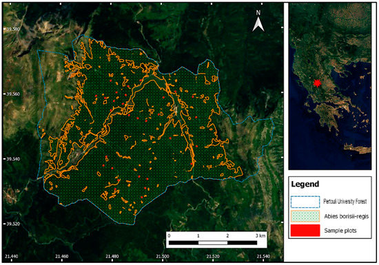
Figure 1.
Map of the study area, including the sample plots’ location and the boundaries of the Abies borisii-regis cover.
Abies borisii-regis constitutes the dominant species of the forest covering almost 90% of the area. It is a tall evergreen coniferous species of the Pinaceae family and a natural hybrid between Abies alba and Abies cephalonica [50]. The forest is characterized by naturally regenerated multi-layered stands, with a dense understory, due to the shade-tolerant properties of the Abies species. Even-aged trees can have different heights and stem diameters, mainly due to tree-to-tree competition and soil quality properties [8,51].
2.2. Field Data Collection and Total Stem Biomass Calculation
Field TSB measurements were conducted in 2018 and composed of two steps. The first included the DBH and tree height measurements in each plot, while in the second step, an allometric equation was employed for the plot-level TSB estimation.
More specifically, DBH and tree height field data were collected from 30 sample plots, each of which covered an area of 1000 m2 (rectangle with dimensions 25 × 40 m). The selection of the specific plot dimensions was based on the official sampling method adopted in the framework of the Pertouli University Forest management plan development. The distribution of the plots over the entire study area was based on different forest conditions (i.e., topography and vegetation density). Next, the allometric equation developed by Georgopoulos et al. (2021) was employed for the calculation of the TSB in each plot. More specifically, the TSB allometric equation was developed, employing 32 destructively sampled trees, using ordinary least square regression and primarily based on DBH (Table 1).

Table 1.
Parameter values, residual standard error, R2, and adjusted R2 for total stem biomass estimation based on DBH.
The development of the allometric model was solely based on DBH, to eliminate possible inaccuracies in the tree height measurements [52]. The calculated TSB varied between 3.3 Mg/1000 m2 and 10.3 Mg/1000 m2 (Figure 2).
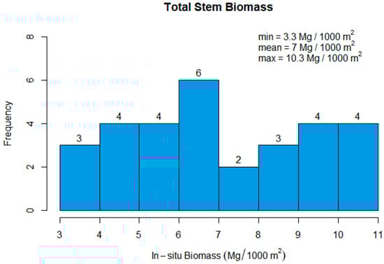
Figure 2.
Total stem biomass (TSB) distribution over the sample plots.
2.3. Satellite Data
SAR data comprised a single Sentinel-1B C-band image acquired from the European Space Agency (ESA) Copernicus Access Hub (https://scihub.copernicus.eu/, (accessed on 13 November 2022), which provides free access to Sentinel products. It is a ground range detected high resolution (GRDH) and dual-polarized VV/VH image, acquired in the interferometric wide (IW) swath mode of the sensor. The selection of the acquisition date (i.e., 22 July 2018) was based on the time of field work, on the meteorological data produced by the National Observatory of Athens, and the orbit passing time, so that rainfall and humidity effects on the backscatter values were avoided. Meteorological data indicated a 10 day no-rain period before the acquisition date and the descending orbit passing time of the image was 16:30, indicating less relative humidity compared to the ascending orbit with a passing time of 04:39.
Optical data consisted of a single Sentinel-2A L2A Multispectral Instrument (MSI) image acquired on 23 July 2018. This acquisition date was selected based on the cloud cover, as well as the growing season and flowering of Abies borisii-regis species (Table 2).
Table 2.
Satellite imagery type, acquisition date, and orbit used for the TSB estimation.
2.4. Methodology
The methodology for the Sentinel-1 and Sentinel-2-based TSB estimation was composed of three parts, namely the Sentinel-1 processing and feature extraction, the Sentinel-2 processing and feature extraction, and the RF modelling and assessment. Figure 3 provides a flowchart of the entire workflow, which is described in detail in the following sections (Section 2.4.1, Section 2.4.2 and Section 2.4.3).
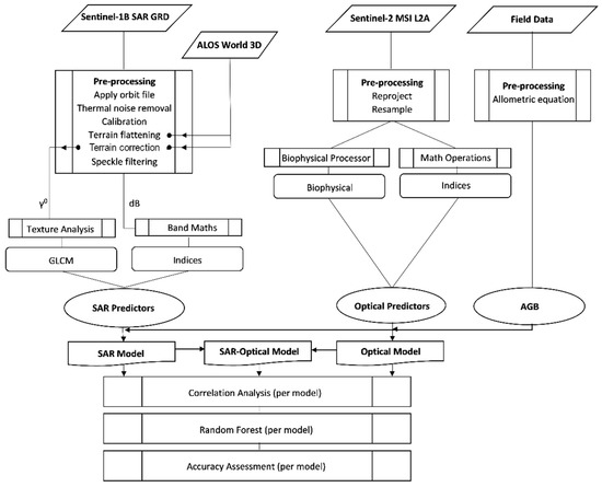
Figure 3.
Flowchart of the workflow employed for the plot-level TSB (total stem biomass) estimation using Sentinel-1, -2 data, and RF modelling.
2.4.1. Sentinel-1 Processing and Feature Extraction
Sentinel-1 image preprocessing was conducted in the Sentinel Application Platform (SNAP) v.8, in six major steps (i.e., orbit file application, thermal noise removal, radiometric calibration, terrain flattening, terrain correction, and speckle filtering). Thermal denoising reduces the impact of the noise induced by the background energy of the SAR instrument, especially in the cross-polarization channel (i.e., VH), and thus improves the quality of the Level 1 image [53,54]. Radiometric calibration was performed to convert the SAR data pixel values (stored as digital numbers) to radiometrically calibrated beta (b0) naught backscatter values. Due to the intense topography of the study area (average slope = 17.87%), terrain variations affected the brightness of the radar return, and slopes facing the sensor appeared brighter (higher backscatter) than the opposite ones (lower backscatter). Therefore, terrain flattening was performed using a digital elevation model (DEM), to correct the radiometric distortions caused by different local incidence angles. This correction converted b0 backscatter values to terrain-flattened gamma naught (γ0) values. Subsequently, terrain correction was applied to convert radar viewing geometry to a geographic projection (UTM 34N) and specify the output pixel size (10 m × 10 m).
For both aforementioned steps, namely, the terrain flattening and terrain correction, the Advanced Land Observing Satellite (ALOS) World 3D 30 m DEM was employed, since it presents the highest accuracy among the freely available DEMs [55,56]. Finally, Frost speckle filtering with a five by five kernel window size was applied to the terrain and radiometrically corrected the image, to reduce the granular noise, known as speckles. The Frost filter has been demonstrated to be one of the best speckle filters for retrieving biophysical parameters such as forest AGB [57]. Once the speckles were reduced, linear γ0 backscatter values were converted in decibel (dB) using logarithmic transformation.
A variety of studies have shown the close relationship of polarization channels and texture images with forest AGB (more details presented in Section 1) [58,59,60]. Therefore, six polarization indices were computed based on the decibelized result of the backscatter coefficient of the vertical transmit-horizontal (VHdB) and vertical transmit-vertical (VVdB) channel, and used as additional predictor variables (Table 3). Moreover, the orthorectified image of each polarization, γ0 VH, and γ0 VV, was used as the input image for generating texture features, to avoid any potential loss of texture information from speckle reduction [61]. Texture expresses the spatial distribution of grayscale characteristics in the image and plays a vital role in pattern recognition [62]. Image textures were calculated using the Grey Level Co-occurrence Matrix (GLCM) tool in SNAP, with an eleven by eleven moving window. As a result, ten different texture variables were computed for each polarization, namely contrast, dissimilarity, homogeneity, angular second moment-ASM, energy, entropy, mean, max, variance, and correlation (Table 3):
Table 3.
List of Sentinel-1 predictors used for the aboveground biomass (AGB) modelling (γ0 represents the terrain-flattened gamma naught values).
2.4.2. Sentinel-2 Processing and Feature Extraction
The Sentinel-2A L2A imagery was downloaded within the Google Earth Engine (GEE) environment. The Level-2A products were already atmospherically corrected, providing bottom of atmosphere (BOA) reflectance images [63]. Among the multispectral bands of Sentinel-2, the 20 m resolution bands covering the red edge (RE), near-infrared (NIR), and short-wave infrared (SWIR) part of the spectrum were resampled to 10 m resolution using a bilinear resampling algorithm.
Considering that a close relationship was found in previous studies between optical sensors’ spectral products (e.g., vegetation indices) and forest AGB [16,17,18,19,20,64], eight broad- and narrow-band greenness vegetation indices, one water content vegetation index, and three biophysical parameters (i.e., leaf area index (LAI), fraction of absorbed photosynthetically active radiation (FAPAR), fractional cover (FCOVER)) were computed and employed as additional predictor variables (Table 4). Spectral feature selection was based on their merits for biophysical parameter retrieval, as identified in recent studies [9,11,19,32]. Vegetation index computation was performed within the GGE environment, while biophysical parameters were produced using the biophysical processor tool of the SNAP toolbox. Similarly to the Sentinel-1 predictors, the arithmetic means of the aforementioned predictors were employed in each plot for the TSB estimation.
Table 4.
List of Sentinel-2 predictors used for the aboveground biomass (AGB) modeling.
2.4.3. Random Forest Modelling and Accuracy Assessment
RF is an ensemble technique that uses multiple decision trees to perform classification and, in this case, regression tasks [65]. Each decision tree is trained on a different subset of the input data with data replacement, a technique called bagging or bootstrap aggregation [65]. Predictions of each regression tree aggregate, by taking their mean, to produce a final predictive model [66]. The bagging technique occurs on two-thirds of the input data, while the remaining one-third, called out-of-bag (OOB) data, contributes to the calculation of the mean prediction error (out-of-bag error) [66].
Considering that the use of highly correlated or redundant predictors may increase the complexity and uncertainty of a prediction model, Pearson’s correlation [67] was employed for each dataset (i.e., Sentinel-1, Sentinel-2, and their combination), in order to identify any linear relationship between the predictor variables and field-measured TSB. The “findCorrelation” function provided within the caret package [68] was used for each dataset, to remove one of the two identified variables that had a linear correlation higher than 0.9.
After removing the strongly correlated features, three different RF models were produced and examined for their potential to reliably predict TSB data. The first predictive model was based on the Sentinel-1 image and its derivatives, namely polarization indices and texture images (hereafter referred as the SAR model); the second was based on the Sentinel-2 image and products, namely vegetation indices and biophysical parameters, (hereafter referred as the optical model); and the last was developed using a combination of Sentinel-1 and -2 predictor variables (hereafter referred as the SAR–optical model). All three models were generated in R using the randomForest [69] and caret packages. Concerning RF tuning, two hyperparameters were tuned using a grid search, namely the number of trees to grow and the number of predictors for each tree. The number of trees to be grown varied from 50 to 500, with a step of 50, and the number of selected predictors was defined as the number of predictors divided by three.
The reliability of the developed predictive models was assessed using a 10 fold cross-validation (CV) (as suggested by Hastie et al. (2001) [65] for small sampling sizes) repeated three times. In each repetition of the 10 fold CV, the original dataset was split into ten subsets (folds), the model was trained on nine of them, while the remaining subset was used to validate the model’s performance. This operation was repeated ten times (i.e., one per validation subset), producing ten performance scores, the average of which defined the model’s performance for each repetition. Finally, the models’ accuracy was derived by computing the cross-validated metrics of the coefficient of determination (R2) (Equation (1)), the root mean square error (RMSE) (Equation (2)), and the mean absolute error (MAE) (Equation (3)):
where is the measured TSB for plot , is the predicted TSB for plot , is the mean measured TSB, and the number of observations (i.e., the number of sample plots).
3. Results
3.1. Correlation Analysis
The results of the application of Pearson’s correlation for the removal of inter-correlated variables are presented in Figure 4. In particular, this figure depicts the Pearson’s correlation matrix of all variables that remained after the collinearity rejection. Among the Sentinel-1 predictors, the VH_GLCMVariance texture achieved the highest positive correlation, with field-measured TSB obtaining an r-value of 0.48. This was followed by Pol_mean index and VH_MAX texture, with r-values of 0.35 and 0.34, respectively. Accordingly, among the Sentinel-2 predictors, the B11 spectral band achieved the highest negative correlation, with field-measured TSB r = −0.5, followed by NDVIre and NDWI with positive correlations of 0.4 and 0.39, respectively. In addition, a stronger relationship between the spectral bands and indices was observed, compared to the polarization channels and indices.
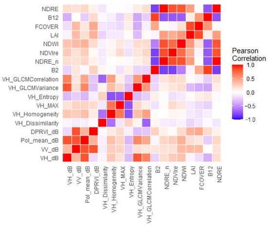
Figure 4.
Pearson’s correlation matrix between the predictor variables and field-measured total stem biomass (TSB) after collinearity rejection.
3.2. Total Stem Biomass Modelling
The performance of the developed RF models for TSB estimation using Sentinel-1, Sentinel-2, and their combination is presented in Table 5. In particular, among the employed single-sensor approaches, the developed SAR model provided a better performance for TSB estimation (i.e., R2 = 0.74, RMSE = 1.76 Mg/1000 m2, MAE = 1.48 Mg/1000 m2), compared to the optical model (i.e., R2 = 0.63, RMSE = 2.19 Mg/1000 m2 and MAE = 1.89 Mg/1000 m2). The SAR–optical model marginally underperformed compared to the SAR model, presenting an R2 of 0.73, an RMSE of 1.92 Mg/1000 m2, and an MAE equal to 1.63 Mg/1000 m2. Figure 5 depicts the performance of the developed regression models using scatterplots, explaining the relationship between the field-measured and predicted TSB values.
Table 5.
Cross-validation metrics derived separately for the models developed using Sentinel-1 and Sentinel-2 data and their combination.
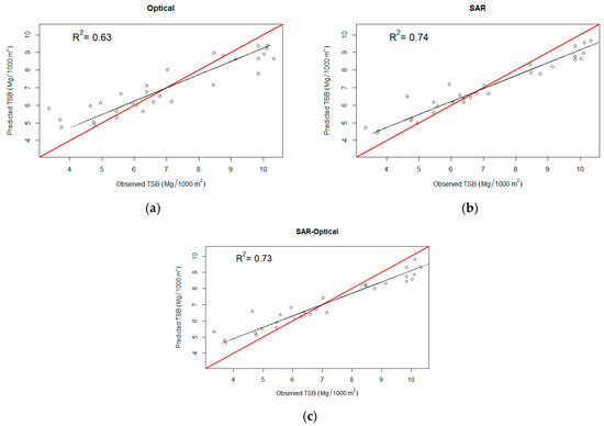
Figure 5.
Predicted vs. measured biomass graph for the developed (a) optical, (b) SAR, and (c) SAR–optical predictive models for total stem biomass (TSB) estimation. The black line represents the fitted line, and the red line represents the 1:1 line.
With regard to the relative predictors’ importance for the TSB estimation (Figure 6), the SAR model indicated that VH_GLCMVariance was the most important variable, followed by the VH_MAX, VH polarization channel and Pol_mean. The VH_GLCMVariance texture was also considered the most important variable for the SAR–optical model, followed by the NDVI index and VH polarization channels (VH_dB and VH_MAX). Regarding the optical model, the B11 spectral band, which was highly correlated with B12 (r = 0.99), was identified as the most important variable, presenting the highest frequency of occurrence, followed by the NDVIre, B2, and NDWI indices.
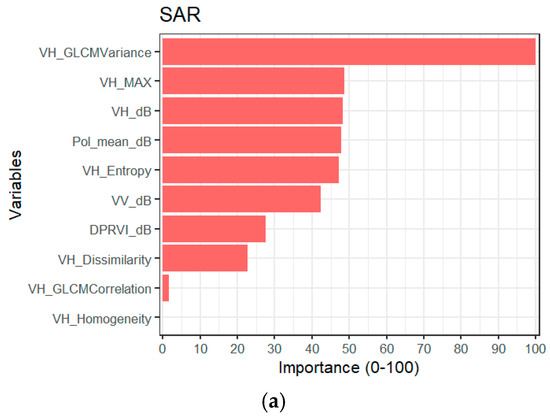
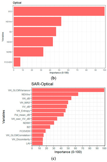
Figure 6.
Predictors’ importance for each developed regression model (i.e., (a) SAR, (b) optical, (c) SAR–optical).
4. Discussion
In this study, SAR and optical satellite data were evaluated for their potential in reliable TSB estimation in an uneven-aged structured coniferous forest (Abies borisii-regis), characterized by a dense canopy and topographically complex terrain. More specifically, Sentinel-1 and -2 images were employed in an individual and combined manner for the estimation of TSB at the plot-level, using RF modelling. As a result, three predictive models (i.e., SAR, optical, and SAR–optical) were developed and evaluated for their accuracy using field measurements and the k-fold CV method. SAR backscatter, SAR image texture, spectral bands, and spectral vegetation indices were used as predictor variables for the RF models’ development, considering that each of them reflects different properties of the tree canopy. The predictive performance of the developed models was evaluated using the 10 fold CV method and intercompared. Overall, the results showcased that the individual use of the Sentinel-1 data contributed to the production of the most accurate plot-level TSB estimates, compared to the use of Sentinel-2 data individually and the Sentinel-1 and -2 combination. In fact, the synergistic use of optical and SAR data led to the generation of an RF model which only marginally underperformed the SAR model (R2 = 0.73 and R2 = 0.72, respectively).
Regarding the Sentinel-2 variable importance in the plot-level TSB estimation, the results of this work showed that the SWIR band (i.e., B11) was the variable of highest importance in our study area, which is characterized by a dense multi-layered canopy and intense topography (Figure 6b). This is consistent with previous research that indicated a strong correlation between SWIR and biomass, especially in areas with complicated stand canopy structures, such as in our area of interest [70]. For instance, Lu et al. (2004) examined the relationships between spectral responses (e.g., bands, indices, transformed images) and biomass in three study areas in the Brazilian Amazon with various forest conditions and soil properties [71]. The research concluded that in complex stand structures SWIR-based vegetation indices have a stronger relationship with biomass than NIR. Accordingly, in the research results of Wang et al. (2021), the SWIR band (i.e., B12) presented a stronger correlation with AGB than the other spectral bands, due to its strong ability to reflect the complexity of the forest stand structure [72]. In addition, SWIR contributes to biomass estimation, since it reflects the moisture content of vegetation and presents a lower sensitivity to atmospheric conditions compared to the other spectral bands [71,72,73,74].
As far as the Sentinel-1 variables are concerned, SAR texture, namely the VH_GLCMVariance, showed the highest explanatory power in the respective TSB predictive model (Figure 6a). This can be attributed to the fact that texture parameters are more effective in TSB estimation over areas of high local variance [75] and provide more information in forests with multiple layers and complex structures, as in our case [76]. Argamosa et al. (2018) examined the AGB modelling of mangrove forest using Sentinel-1 indices and texture, and found VH_GLCMVariance to be the best performing variable [31]. However, Zhao et al. (2016) found that textures depend on the vegetation types and remote sensing data sources and that no single texture is optimal for biomass estimation in different study areas [77]. According to the results of our study, the texture features (e.g., VH_GLCMVariance, VH_MAX, and VH_Entropy) were identified as the most significant variables for TSB estimation compared to the spectral bands, which agrees with Lu (2005), who found that texture images present a better performance than spectral bands in biomass estimation (i.e., R2 = 0.708 and 0.404, respectively), particularly for forests with complex stand structures [78]. On the contrary, this was not the case in the study of Ghosh and Behera (2018) conducted over homogeneous sites, where the SAR texture presented a lower performance than vegetation indices [17].
A saturation effect can be observed in the scatterplots of Figure 5 for plots where the biomass was over 7.5 Mg/1000 m2, which applies to all three predictive models (i.e., the SAR, the optical, and the SAR–optical model). This can be attributed to the inability of optical sensors to directly measure bole biomass (i.e., trunk and branches), which intensifies in dense mature forests, where even less information about the uppermost part of the canopy can be retrieved from spectral responses [59,79]. As a consequence, optical-derived predictors underestimate biomass in dense forest stands, while in sparse forest the biomass is overestimated due to the influence of the forest understory [80]. Regarding the Sentinel-1 data, the observed saturation level was also consistent with a previous study that revealed saturation at about 60–70 tons/ha [81]. More specifically, SAR data saturation was a result of C-band’s low penetrating power into the forest canopy [81]. Therefore, in densely forested areas, the sensitivity to biomass remains stagnant after a certain biomass value, leading to its underestimation. Moreover, several factors influence SAR signal saturation, such as vegetation type, soil moisture, especially for low biomass areas, leaf type and presence, weather conditions, canopy unevenness, and SAR polarization [82]. A study on biomass estimation over tropical broadleaf evergreen forests in Hawaii and coniferous forests in North America and Europe reported higher saturation levels of around 20 tons/ha for C-band for both forest types [83]. In order to extend the saturation levels of backscatter at higher biomass values, we made use of texture images that do not depend on backscatter itself but instead local variance and that thus can be more sensitive to mature heterogeneous forests [17]. However, in order to evaluate the saturation points of the study area with higher confidence, a larger sample size should be examined in the future.
With regard to the predictive performance of the developed RF models, the CV results indicated the superiority of the SAR model (i.e., R2 = 0.74, RMSE = 1.76 Mg/1000 m2, MAE = 1.48 Mg/1000 m2) over the models produced using the optical and SAR–optical data (R2 = 0.63, RMSE = 2.19 Mg/1000 m2, and MAE = 1.89 Mg/1000 m2; and R2 = 0.73, RMSE = 1.92 Mg/1000 m2, and MAE = 1.63 Mg/1000 m2, respectively). The combination of SAR and optical products also effectively, and only marginally worse compared to the individual use of Sentinel-1, captured the information of multi-layered stand structure. Nevertheless, among the single-sensor approaches, SAR performed noticeably better than the optical model. This finding is consistent with previous studies that used Sentinel-based predictors for biomass estimation. More specifically, a revised study for the Mediterranean region [84] agreed with our findings, stating that biomass estimates based on optical sensors present lower accuracy (R2 ≈ 0.70) than those conducted with radar sensors (R2 ≥ 0.80). Furthermore, Chrysafis et al. (2017) examined the relationships between growing stock volume (GSV) and Sentinel-2 products (bands and vegetation indices) in a mixed Mediterranean forest dominated by black pine, oaks, and beech trees, using an RF model [85]. Although the direct comparison of regression analysis results derived from different studies requires particular caution, it is worth mentioning that the R2 between the GSV and Sentinel-2 of the above research work was calculated to be 0.63, which is almost identical to the respective result in our study. However, the majority of the existing literature in biomass estimation [17,20,32,64,86,87] has made the opposite conclusion (i.e., the optical data overperformed the SAR in biomass estimation). The reason for this major deviation in research findings may be related to the different ecosystems under investigation. For instance, a significant part of the existing literature refers to tropical biomes [84], which are characterized by much higher air humidity, compared to Mediterranean ones, as well as plain terrain, resulting in a higher SAR signal saturation and unhindered recording of the canopy surface by the optical sensor.
Despite the fact that our study achieved its aims, there were some noteworthy and unavoidable limitations. Although the selection of plots was based on different forest conditions, so that the samples were as representative as possible, the sample size could be characterized as rather limited. As such, the reliability of the predictive models was assessed using the k-fold CV method, as suggested by Hastie et al. (2001) [65], to remove overfitting and avoid additional uncertainty in the predictions [88]. Overall, the importance of the samples capturing the biomass variability across the study area gained the most attention in our work and was considered a priority [34]. Finally, it should also be noted that the application of the developed predictive models to ecosystems of different vegetation compositions and topographic conditions would negatively influence the prediction results, since diverse relationships would be identified between the response and LiDAR-derived predictive variables.
5. Conclusions
The present research focused on the investigation of the potential of Sentinel-1 and Sentinel-2 data in estimating plot-level TSB in a dense uneven-aged structured fir forest using RF modelling. Three RF regression models were constructed based on individual and synergistic use of the Sentinel data, and their predictive performance was evaluated using the 10 fold CV approach and inter-compared. The validation results suggested that the combined use of Sentinel-1 data alone contributed best to the reliable prediction of plot-level TSB in our study area, which is characterized by multi-layered canopy and complex terrain. More specifically:
- The RF regression model produced by the individual use of Sentinel-1 data overperformed (R2 = 0.74) those derived from Sentinel-2 and the combination of Sentinel-1 and -2 data (R2 = 0.63 and R2 = 0.73, respectively).
- The predictive performance of the model produced by the synergistic use of Sentinel-1 and Sentinel-2 data was marginally lower than that generated by Sentinel-1 alone (R2 = 0.73, RMSE = 1.92 Mg/1000 m2, and MAE = 1.63 Mg/1000 m2; and R2 = 0.74, RMSE = 1.76 Mg/1000 m2, and MAE = 1.48 Mg/1000 m2, respectively).
- The observed difference in terms of predictive performance between the SAR and the SAR–optical model cannot be considered significant. Consequently, the use of SAR data individually for accurate TSB estimation can be considered more efficient, in terms both of the prediction accuracy and computational time.
- Sentinel-1 texture parameters and the Sentinel-2 SWIR band (B11) were the variables with the highest importance for plot-level TSB estimation.
- Both SAR and optical data presented the limitation of signal saturation when sensing high biomass values. A saturation effect was introduced over 7.5 Mg/1000 m2 for the SAR, optical, and combined RF models.
In summary, the results of the present study suggest the capability of Sentinel-1 and Sentinel-2 data to effectively contribute to TSB estimation using the RF regression method in a forest environment of complex vegetation structure and topography. Nevertheless, the RF model produced using Sentinel-1 data presented a better predictive performance compared to those generated using Sentinel-2 and the synergistic use of Sentinel-1 and -2 data. Considering the limitations of the present study, it would be of great interest to collect more sample plots, in order to validate the results. Further research could also examine ANNs and XGBoost approaches in estimating TSB at the plot-level in our study area.
Author Contributions
Conceptualization, N.G., A.S. and I.Z.G.; Methodology, C.S., N.G. and A.S.; Software, N.G.; Validation, C.S. and N.G.; Formal analysis, N.G. and C.S.; Investigation, C.S. and N.G.; Resources, I.Z.G.; Data curation, A.S.; Writing—original draft preparation, C.S. and A.S.; Writing—review and editing, A.S., N.G. and I.Z.G.; Visualization, C.S.; Supervision, I.Z.G.; Project administration, I.Z.G. All authors have read and agreed to the published version of the manuscript.
Funding
This research received no external funding. The APC was funded by the Laboratory of Forest Management and Remote Sensing, School of Forestry and Natural Environment, Aristotle University of Thessaloniki.
Institutional Review Board Statement
Not applicable.
Informed Consent Statement
Not applicable.
Data Availability Statement
Not applicable.
Conflicts of Interest
The authors declare no conflict of interest.
References
- Wani, A.A.; Joshi, P.K.; Singh, O. Estimating Biomass and Carbon Mitigation of Temperate Coniferous Forests Using Spectral Modeling and Field Inventory Data. Ecol. Inform. 2015, 25, 63–70. [Google Scholar] [CrossRef]
- Hoover, K.; Riddle, A.A. Forest Carbon Primer; Congressional Research Service: Washington, DC, USA, 2020. [Google Scholar]
- Yusuf, H.A.; Oludipe, J.J.; Adeoye, O.O.; Olorunfemi, I.E. Carbon Stocks in Aboveground and Belowground Biomass of Sub-Humid Tropical Forest in Southwestern Nigeria. Open Access Libr. J. 2019, 6, 1–12. [Google Scholar] [CrossRef]
- Ravindranath, N.H.; Ostwald, M. Methods for Estimating Above-Ground Biomass. In Carbon Inventory Methods: Handbook for Greenhouse Gas Inventory, Carbon Mitigation and Roundwood Production Projects; Springer: Berlin/Heidelberg, Germany, 2008. [Google Scholar]
- Cairns, M.A.; Brown, S.; Helmer, E.H.; Baumgardner, G.A. Root Biomass Allocation in the World’s Upland Forests. Oecologia 1997, 111, 1–11. [Google Scholar] [CrossRef]
- Chen, L.; Ren, C.; Zhang, B.; Wang, Z.; Xi, Y. Estimation of Forest Above-Ground Biomass by Geographically Weighted Regression and Machine Learning with Sentinel Imagery. Forests 2018, 9, 582. [Google Scholar] [CrossRef]
- Sessa, R.; Dolman, H. Terrestrial essential climate variables for climate change assessment, mitigation and adaptation. FAO/GTOS 2008, 44. [Google Scholar]
- Georgopoulos, N.; Gitas, I.Z.; Stefanidou, A.; Korhonen, L.; Stavrakoudis, D. Estimation of Individual Tree Stem Biomass in an Uneven-Aged Structured Coniferous Forest Using Multispectral LiDAR Data. Remote Sens. 2021, 13, 4827. [Google Scholar] [CrossRef]
- Lourenço, P. Biomass Estimation Using Satellite-Based Data. Forest Biomass-From Trees to Energy; IntechOpen: London, UK, 2021. [Google Scholar]
- Deo, R.K.; Domke, G.M.; Russell, M.B.; Woodall, C.W.; Andersen, H.-E. Evaluating the Influence of Spatial Resolution of Landsat Predictors on the Accuracy of Biomass Models for Large-Area Estimation across the Eastern USA. Environ. Res. Lett. 2018, 13, 055004. [Google Scholar] [CrossRef]
- Mauya, E.W.; Madundo, S. Modelling and Mapping Above Ground Biomass Using Sentinel 2 and Planet Scope Remotely Sensed Data in West Usambara Tropical Rainforests, Tanzania. Res. Sq. 2021. Preprint. [Google Scholar] [CrossRef]
- Forkuor, G.; Dimobe, K.; Serme, I.; Tondoh, J.E. Landsat-8 vs. Sentinel-2: Examining the Added Value of Sentinel-2’s Red-Edge Bands to Land-Use and Land-Cover Mapping in Burkina Faso. GIScience Remote Sens. 2018, 55, 331–354. [Google Scholar] [CrossRef]
- Qiu, S.; He, B.; Yin, C.; Liao, Z. Assessments of Sentinel-2 Vegetation Red-Edge Spectral Bands For Improving Land Cover Classification. In Proceedings of the the International Archives of the Photogrammetry, Remote Sensing and Spatial Information Sciences, Virtual, 13 September 2017; Copernicus GmbH: Gottingen, Germany; Volume XLII-2-W7, pp. 871–874. [Google Scholar]
- Li, C.; Zhou, L.; Xu, W. Estimating Aboveground Biomass Using Sentinel-2 MSI Data and Ensemble Algorithms for Grassland in the Shengjin Lake Wetland, China. Remote Sens. 2021, 13, 1595. [Google Scholar] [CrossRef]
- Mutanga, O.; Skidmore, A.K. Narrow Band Vegetation Indices Overcome the Saturation Problem in Biomass Estimation. Int. J. Remote Sens. 2004, 25, 3999–4014. [Google Scholar] [CrossRef]
- Pandit, S.; Tsuyuki, S.; Dube, T. Estimating Above-Ground Biomass in Sub-Tropical Buffer Zone Community Forests, Nepal, Using Sentinel 2 Data. Remote Sens. 2018, 10, 601. [Google Scholar] [CrossRef]
- Ghosh, S.M.; Behera, M.D. Aboveground Biomass Estimation Using Multi-Sensor Data Synergy and Machine Learning Algorithms in a Dense Tropical Forest. Appl. Geogr. 2018, 96, 29–40. [Google Scholar] [CrossRef]
- Pham, T.D.; Le, N.N.; Ha, N.T.; Nguyen, L.V.; Xia, J.; Yokoya, N.; To, T.T.; Trinh, H.X.; Kieu, L.Q.; Takeuchi, W. Estimating Mangrove Above-Ground Biomass Using Extreme Gradient Boosting Decision Trees Algorithm with Fused Sentinel-2 and ALOS-2 PALSAR-2 Data in Can Gio Biosphere Reserve, Vietnam. Remote Sens. 2020, 12, 777. [Google Scholar] [CrossRef]
- Jha, N.; Tripathi, N.K.; Barbier, N.; Virdis, S.G.; Chanthorn, W.; Viennois, G.; Brockelman, W.Y.; Nathalang, A.; Tongsima, S.; Sasaki, N. The Real Potential of Current Passive Satellite Data to Map Aboveground Biomass in Tropical Forests. Remote Sens. Ecol. Conserv. 2021, 7, 504–520. [Google Scholar] [CrossRef]
- Forkuor, G.; Zoungrana, J.-B.B.; Dimobe, K.; Ouattara, B.; Vadrevu, K.P.; Tondoh, J.E. Above-Ground Biomass Mapping in West African Dryland Forest Using Sentinel-1 and 2 Datasets-A Case Study. Remote Sens. Environ. 2020, 236, 111496. [Google Scholar] [CrossRef]
- Powell, S.L.; Cohen, W.B.; Healey, S.P.; Kennedy, R.E.; Moisen, G.G.; Pierce, K.B.; Ohmann, J.L. Quantification of Live Aboveground Forest Biomass Dynamics with Landsat Time-Series and Field Inventory Data: A Comparison of Empirical Modeling Approaches. Remote Sens. Environ. 2010, 114, 1053–1068. [Google Scholar] [CrossRef]
- Avitabile, V.; Baccini, A.; Friedl, M.A.; Schmullius, C. Capabilities and Limitations of Landsat and Land Cover Data for Aboveground Woody Biomass Estimation of Uganda. Remote Sens. Environ. 2012, 117, 366–380. [Google Scholar] [CrossRef]
- Achard, F.; Stibig, H.-J.; Eva, H.D.; Lindquist, E.J.; Bouvet, A.; Arino, O.; Mayaux, P. Estimating Tropical Deforestation from Earth Observation Data. Carbon Manag. 2010, 1, 271–287. [Google Scholar] [CrossRef]
- Shimada, M. Ortho-Rectification and Slope Correction of SAR Data Using DEM and Its Accuracy Evaluation. IEEE J. Sel. Top. Appl. Earth Obs. Remote Sens. 2010, 3, 657–671. [Google Scholar] [CrossRef]
- Ban, Y.; Zhang, P.; Nascetti, A.; Bevington, A.R.; Wulder, M.A. Near Real-Time Wildfire Progression Monitoring with Sentinel-1 SAR Time Series and Deep Learning. Sci. Rep. 2020, 10, 1322. [Google Scholar] [CrossRef] [PubMed]
- Ouchi, K. Recent Trend and Advance of Synthetic Aperture Radar with Selected Topics. Remote Sens. 2013, 5, 716–807. [Google Scholar] [CrossRef]
- Lucas, R.; Armston, J.; Fairfax, R.; Fensham, R.; Accad, A.; Carreiras, J.; Kelley, J.; Bunting, P.; Clewley, D.; Bray, S. An Evaluation of the ALOS PALSAR L-Band Backscatter—Above Ground Biomass Relationship Queensland, Australia: Impacts of Surface Moisture Condition and Vegetation Structure. IEEE J. Sel. Top. Appl. Earth Obs. Remote Sens. 2010, 3, 576–593. [Google Scholar] [CrossRef]
- Englhart, S.; Keuck, V.; Siegert, F. Aboveground Biomass Retrieval in Tropical Forests—The Potential of Combined X-and L-Band SAR Data Use. Remote Sens. Environ. 2011, 115, 1260–1271. [Google Scholar] [CrossRef]
- Reiche, J.; Lucas, R.; Mitchell, A.L.; Verbesselt, J.; Hoekman, D.H.; Haarpaintner, J.; Kellndorfer, J.M.; Rosenqvist, A.; Lehmann, E.A.; Woodcock, C.E. Combining Satellite Data for Better Tropical Forest Monitoring. Nat. Clim. Change 2016, 6, 120–122. [Google Scholar] [CrossRef]
- Nasirzadehdizaji, R.; Balik Sanli, F.; Abdikan, S.; Cakir, Z.; Sekertekin, A.; Ustuner, M. Sensitivity Analysis of Multi-Temporal Sentinel-1 SAR Parameters to Crop Height and Canopy Coverage. Appl. Sci. 2019, 9, 655. [Google Scholar] [CrossRef]
- Argamosa, R.J.L.; Blanco, A.C.; Baloloy, A.B.; Candido, C.G.; Dumalag, J.B.L.C.; Dimapilis, L.L.C.; Paringit, E.C. MODELLING ABOVE GROUND BIOMASS OF MANGROVE FOREST USING SENTINEL-1 IMAGERY. ISPRS Ann. Photogramm. Remote Sens. Spat. Inf. Sci. 2018, IV–3, 13–20. [Google Scholar] [CrossRef]
- Ronoud, G.; Fatehi, P.; Darvishsefat, A.A.; Tomppo, E.; Praks, J.; Schaepman, M.E. Multi-Sensor Aboveground Biomass Estimation in the Broadleaved Hyrcanian Forest of Iran. Can. J. Remote Sens. 2021, 47, 818–834. [Google Scholar] [CrossRef]
- Cutler, M.E.J.; Boyd, D.S.; Foody, G.M.; Vetrivel, A. Estimating Tropical Forest Biomass with a Combination of SAR Image Texture and Landsat TM Data: An Assessment of Predictions between Regions. ISPRS J. Photogramm. Remote Sens. 2012, 70, 66–77. [Google Scholar] [CrossRef]
- Fassnacht, F.E.; Neumann, C.; Forster, M.; Buddenbaum, H.; Ghosh, A.; Clasen, A.; Joshi, P.K.; Koch, B. Comparison of Feature Reduction Algorithms for Classifying Tree Species with Hyperspectral Data on Three Central European Test Sites. IEEE J. Sel. Top. Appl. Earth Obs. Remote Sens. 2014, 7, 2547–2561. [Google Scholar] [CrossRef]
- Ou, G.; Li, C.; Lv, Y.; Wei, A.; Xiong, H.; Xu, H.; Wang, G. Improving Aboveground Biomass Estimation of Pinus Densata Forests in Yunnan Using Landsat 8 Imagery by Incorporating Age Dummy Variable and Method Comparison. Remote Sens. 2019, 11, 738. [Google Scholar] [CrossRef]
- Luo, M.; Wang, Y.; Xie, Y.; Zhou, L.; Qiao, J.; Qiu, S.; Sun, Y. Combination of Feature Selection and Catboost for Prediction: The First Application to the Estimation of Aboveground Biomass. Forests 2021, 12, 216. [Google Scholar] [CrossRef]
- Martins-Neto, R.P.; Tommaselli, A.M.G.; Imai, N.N.; David, H.C.; Miltiadou, M.; Honkavaara, E. Identification of Significative LiDAR Metrics and Comparison of Machine Learning Approaches for Estimating Stand and Diversity Variables in Heterogeneous Brazilian Atlantic Forest. Remote Sens. 2021, 13, 2444. [Google Scholar] [CrossRef]
- Belgiu, M.; Drăguţ, L. Random Forest in Remote Sensing: A Review of Applications and Future Directions. ISPRS J. Photogramm. Remote Sens. 2016, 114, 24–31. [Google Scholar] [CrossRef]
- Vauhkonen, J.; Korpela, I.; Maltamo, M.; Tokola, T. Imputation of Single-Tree Attributes Using Airborne Laser Scanning-Based Height, Intensity, and Alpha Shape Metrics. Remote Sens. Environ. 2010, 114, 1263–1276. [Google Scholar] [CrossRef]
- Corte, A.P.D.; Souza, D.V.; Rex, F.E.; Sanquetta, C.R.; Mohan, M.; Silva, C.A.; Zambrano, A.M.A.; Prata, G.; Alves de Almeida, D.R.; Trautenmüller, J.W.; et al. Forest Inventory with High-Density UAV-Lidar: Machine Learning Approaches for Predicting Individual Tree Attributes. Comput. Electron. Agric. 2020, 179, 105815. [Google Scholar] [CrossRef]
- Silveira, E.M.O. Object-Based Random Forest Modelling of Aboveground Forest Biomass Outperforms a Pixel-Based Approach in a Heterogeneous and Mountain Tropical Environment. Int. J. Appl. Earth Obs. Geoinf. 2019, 78, 175–188. [Google Scholar] [CrossRef]
- Schlund, M.; Davidson, M.W.J. Aboveground Forest Biomass Estimation Combining L- and P-Band SAR Acquisitions. Remote Sens. 2018, 10, 1151. [Google Scholar] [CrossRef]
- Lebedev, A.; Kuzmichev, V. Changes of Tree Stem Biomass in European Forests since 1950. J. For. Sci. 2022, 68, 107–115. [Google Scholar] [CrossRef]
- Zhang, L.; Deng, X.; Lei, X.; Xiang, W.; Peng, C.; Lei, P.; Yan, W. Determining Stem Biomass of Pinus Massoniana L. through Variations in Basic Density. Forestry 2012, 85, 601–609. [Google Scholar] [CrossRef]
- Leite, R.V.; Amaral, C.H.D.; Pires, R.D.P.; Silva, C.A.; Soares, C.P.B.; Macedo, R.P.; Silva, A.A.L.D.; Broadbent, E.N.; Mohan, M.; Leite, H.G. Estimating Stem Volume in Eucalyptus Plantations Using Airborne LiDAR: A Comparison of Area- and Individual Tree-Based Approaches. Remote Sens. 2020, 12, 1513. [Google Scholar] [CrossRef]
- Xu, X.; Lin, H.; Liu, Z.; Ye, Z.; Li, X.; Long, J. A Combined Strategy of Improved Variable Selection and Ensemble Algorithm to Map the Growing Stem Volume of Planted Coniferous Forest. Remote Sens. 2021, 13, 4631. [Google Scholar] [CrossRef]
- Tomppo, E.; Antropov, O.; Praks, J. Boreal Forest Snow Damage Mapping Using Multi-Temporal Sentinel-1 Data. Remote Sens. 2019, 11, 384. [Google Scholar] [CrossRef]
- Solberg, S. Estimating Spruce and Pine Biomass with Interferometric X-Band SAR. Remote Sens. Environ. 2010, 114, 2353–2360. [Google Scholar] [CrossRef]
- Rahman, M.M.; Tetuko Sri Sumantyo, J. Retrieval of Tropical Forest Biomass Information from ALOS PALSAR Data. Geocarto Int. 2013, 28, 382–403. [Google Scholar] [CrossRef]
- Burkhart, H.E.; Tomé, M. Modeling Forest Trees and Stands; Springer Science & Business Media: Berlin/Heidelberg, Germany, 2012; ISBN 978-90-481-3170-9. [Google Scholar]
- Dobrowolska, D.; Bončina, A.; Klumpp, R. Ecology and Silviculture of Silver Fir (Abies Alba Mill.): A Review. J. For. Res. 2017, 22, 326–335. [Google Scholar] [CrossRef]
- Romero, F.M.B.; Jacovine, L.A.G.; Ribeiro, S.C.; Torres, C.M.M.E.; Silva, L.F.D.; Gaspar, R. de O.; Rocha, S.J.S.S. da; Staudhammer, C.L.; Fearnside, P.M. Allometric Equations for Volume, Biomass, and Carbon in Commercial Stems Harvested in a Managed Forest in the Southwestern Amazon: A Case Study. Forests 2020, 11, 874. [Google Scholar] [CrossRef]
- Freeman, A. SAR Calibration: An Overview. IEEE Trans. Geosci. Remote Sens. 1992, 30, 1107–1121. [Google Scholar] [CrossRef]
- Weiß, T. SenSARP Documentation 2022. Available online: https://readthedocs.org/projects/multiply-sar-pre-processing/downloads/pdf/latest/ (accessed on 13 November 2022).
- Li, H.; Zhao, J. Evaluation of the Newly Released Worldwide AW3D30 DEM Over Typical Landforms of China Using Two Global DEMs and ICESat/GLAS Data. IEEE J. Sel. Top. Appl. Earth Obs. Remote Sens. 2018, 11, 4430–4440. [Google Scholar] [CrossRef]
- Florinsky, I.V.; Skrypitsyna, T.N.; Luschikova, O.S. Comparative Accuracy of the AW3D30 DSM, ASTER GDEM, and SRTM1 DEM: A Case Study on the Zaoksky Testing Ground, Central European Russia. Remote Sens. Lett. 2018, 9, 706–714. [Google Scholar] [CrossRef]
- Giri Ananto, W.H.; Putri, A.F.S.; Hadi, H.A.; Hanum, D.N.; Wiryawan, B.K.P.; Prabaswara, R.R.; Arjasakusuma, S. Performance of Various Speckle Filter Methods in Modelling Forest Aboveground Biomass Using Sentinel-1 Data: Case Study of Barru Regency, South Sulawesi. In Proceedings of the Sixth Geoinformation Science Symposium, Yogyakarta, Indonesia, 21 November 2019; Wibowo, S.B., Rimba, A.B., Aziz, A., Phinn, S., Sri Sumantyo, J.T., Widyasamratri, H., Arjasakusuma, S., Eds.; SPIE: Yogyakarta, Indonesia, 2019; p. 38. [Google Scholar]
- Prakash, A.J.; Behera, M.D.; Ghosh, S.M.; Das, A.; Mishra, D.R. A New Synergistic Approach for Sentinel-1 and PALSAR-2 in a Machine Learning Framework to Predict Aboveground Biomass of a Dense Mangrove Forest. Ecol. Inform. 2022, 72, 101900. [Google Scholar] [CrossRef]
- Li, H.; Kato, T.; Hayashi, M.; Wu, L. Estimation of Forest Aboveground Biomass of Two Major Conifers in Ibaraki Prefecture, Japan, from PALSAR-2 and Sentinel-2 Data. Remote Sens. 2022, 14, 468. [Google Scholar] [CrossRef]
- Sarker, M.L.R.; Nichol, J.; Ahmad, B.; Busu, I.; Rahman, A.A. Potential of Texture Measurements of Two-Date Dual Polarization PALSAR Data for the Improvement of Forest Biomass Estimation. ISPRS J. Photogramm. Remote Sens. 2012, 69, 146–166. [Google Scholar] [CrossRef]
- Chen, S.; Useya, J.; Mugiyo, H. Decision-Level Fusion of Sentinel-1 SAR and Landsat 8 OLI Texture Features for Crop Discrimination and Classification: Case of Masvingo, Zimbabwe. Heliyon 2020, 6, e05358. [Google Scholar] [CrossRef]
- Tavasoli, N.; Arefi, H. Comparison of Capability of SAR and Optical Data in Mapping Forest above Ground Biomass Based on Machine Learning. Environ. Sci. Proc. 2020, 5, 13. [Google Scholar] [CrossRef]
- European Space Agency. Sentinel-2 User Handbook; European Space Agency: Paris, France, 2015. [Google Scholar]
- Nuthammachot, N.; Askar, A.; Stratoulias, D.; Wicaksono, P. Combined Use of Sentinel-1 and Sentinel-2 Data for Improving above-Ground Biomass Estimation. Geocarto Int. 2022, 37, 366–376. [Google Scholar] [CrossRef]
- Hastie, T.; Friedman, J.; Tibshirani, R. The Elements of Statistical Learning; Springer Series in Statistics; Springer: New York, NY, USA, 2001; ISBN 978-1-4899-0519-2. [Google Scholar]
- Breiman, L. Bagging Predictors. Mach Learn 1996, 24, 123–140. [Google Scholar] [CrossRef]
- Benesty, J.; Chen, J.; Huang, Y.; Cohen, I. Pearson Correlation Coefficient. In Noise Reduction in Speech Processing; Springer Topics in Signal Processing; Springer: Berlin/Heidelberg, Germany, 2009; Volume 2, pp. 1–4. ISBN 978-3-642-00295-3. [Google Scholar]
- Kuhn, M. Building Predictive Models in R Using the Caret Package. J. Stat. Softw. 2008, 28, 1–26. [Google Scholar] [CrossRef]
- Liaw, A.; Wiener, M. Classification and Regression by RandomForest. R News 2002, 2, 5. [Google Scholar]
- Gao, Y.; Lu, D.; Li, G.; Wang, G.; Chen, Q.; Liu, L.; Li, D. Comparative Analysis of Modeling Algorithms for Forest Aboveground Biomass Estimation in a Subtropical Region. Remote Sens. 2018, 10, 627. [Google Scholar] [CrossRef]
- Lu, D.; Mausel, P.; Brondıízio, E.; Moran, E. Relationships between Forest Stand Parameters and Landsat TM Spectral Responses in the Brazilian Amazon Basin. For. Ecol. Manag. 2004, 198, 149–167. [Google Scholar] [CrossRef]
- Wang, Y.; Zhang, X.; Guo, Z. Estimation of Tree Height and Aboveground Biomass of Coniferous Forests in North China Using Stereo ZY-3, Multispectral Sentinel-2, and DEM Data. Ecol. Indic. 2021, 126, 107645. [Google Scholar] [CrossRef]
- Nandy, S.; Singh, R.; Ghosh, S.; Watham, T.; Kushwaha, S.P.S.; Kumar, A.S.; Dadhwal, V.K. Neural Network-Based Modelling for Forest Biomass Assessment. Carbon Manag. 2017, 8, 305–317. [Google Scholar] [CrossRef]
- Zhao, P.; Lu, D.; Wang, G.; Wu, C.; Huang, Y.; Yu, S. Examining Spectral Reflectance Saturation in Landsat Imagery and Corresponding Solutions to Improve Forest Aboveground Biomass Estimation. Remote Sens. 2016, 8, 469. [Google Scholar] [CrossRef]
- Woodcock, C.E.; Strahler, A.H. The Factor of Scale in Remote Sensing. Remote Sens. Environ. 1987, 21, 311–332. [Google Scholar] [CrossRef]
- Han, H.; Wan, R.; Li, B. Estimating Forest Aboveground Biomass Using Gaofen-1 Images, Sentinel-1 Images, and Machine Learning Algorithms: A Case Study of the Dabie Mountain Region, China. Remote Sens. 2022, 14, 176. [Google Scholar] [CrossRef]
- Zhao, P.; Lu, D.; Wang, G.; Liu, L.; Li, D.; Zhu, J.; Yu, S. Forest Aboveground Biomass Estimation in Zhejiang Province Using the Integration of Landsat TM and ALOS PALSAR Data. Int. J. Appl. Earth Obs. Geoinf. 2016, 53, 1–15. [Google Scholar] [CrossRef]
- Lu, D. Aboveground Biomass Estimation Using Landsat TM Data in the Brazilian Amazon. Int. J. Remote Sens. 2005, 26, 2509–2525. [Google Scholar] [CrossRef]
- Isbaex, C.; Coelho, A.M. The Potential of Sentinel-2 Satellite Images for Land-Cover/Land-Use and Forest Biomass Estimation: A Review; IntechOpen: London, UK, 2021; ISBN 978-1-83962-971-6. [Google Scholar]
- Li, C.; Li, M.; Li, Y.; Qian, P. Estimating Aboveground Forest Carbon Density Using Landsat 8 and Field-Based Data: A Comparison of Modelling Approaches. Int. J. Remote Sens. 2020, 41, 4269–4292. [Google Scholar] [CrossRef]
- Nizalapur, V.; Jha, C.; Madugundu, R. Estimation of above Ground Biomass in Indian Tropical Forested Area Using Multi-Frequency DLR-ESAR Data. Int. J. Geomat. Geosci. 2010, 1, 167–178. [Google Scholar]
- Laurin, G.V.; Balling, J.; Corona, P.; Mattioli, W.; Papale, D.; Puletti, N.; Rizzo, M.; Truckenbrodt, J.; Urban, M. Above-Ground Biomass Prediction by Sentinel-1 Multitemporal Data in Central Italy with Integration of ALOS2 and Sentinel-2 Data. J. Appl. Rem. Sens. 2018, 12, 016008. [Google Scholar] [CrossRef]
- Imhoff, M.L. Radar Backscatter and Biomass Saturation: Ramifications for Global Biomass Inventory. IEEE Trans. Geosci. Remote Sens. 1995, 33, 511–518. [Google Scholar] [CrossRef]
- Galidaki, G.; Zianis, D.; Gitas, I.; Radoglou, K.; Karathanassi, V.; Tsakiri–Strati, M.; Woodhouse, I.; Mallinis, G. Vegetation Biomass Estimation with Remote Sensing: Focus on Forest and Other Wooded Land over the Mediterranean Ecosystem. Int. J. Remote Sens. 2017, 38, 1940–1966. [Google Scholar] [CrossRef]
- Chrysafis, I.; Mallinis, G.; Siachalou, S.; Patias, P. Assessing the Relationships between Growing Stock Volume and Sentinel-2 Imagery in a Mediterranean Forest Ecosystem. Remote Sens. Lett. 2017, 8, 508–517. [Google Scholar] [CrossRef]
- Li, Y.; Li, M.; Li, C.; Liu, Z. Forest Aboveground Biomass Estimation Using Landsat 8 and Sentinel-1A Data with Machine Learning Algorithms. Sci Rep 2020, 10, 9952. [Google Scholar] [CrossRef]
- Theofanous, N.; Chrysafis, I.; Mallinis, G.; Domakinis, C.; Verde, N.; Siahalou, S. Aboveground Biomass Estimation in Short Rotation Forest Plantations in Northern Greece Using ESA’s Sentinel Medium-High Resolution Multispectral and Radar Imaging Missions. Forests 2021, 12, 902. [Google Scholar] [CrossRef]
- Lever, J.; Krzywinski, M.; Altman, N. Points of Significance: Model Selection and Overfitting. Nat. Methods 2016, 13, 703–704. [Google Scholar] [CrossRef]
Publisher’s Note: MDPI stays neutral with regard to jurisdictional claims in published maps and institutional affiliations. |
© 2022 by the authors. Licensee MDPI, Basel, Switzerland. This article is an open access article distributed under the terms and conditions of the Creative Commons Attribution (CC BY) license (https://creativecommons.org/licenses/by/4.0/).