Abstract
The hydrological connectivity below the soil surface can influence the forest structure and function, especially soil and plant productivity. However, few studies have determined the changes in the hydrological connectivity below the soil surface with increasing soil depth and have quantified the effects of root systems on the hydrological connectivity in forest ecosystems. In this study, we evaluated the index of the hydrological connectivity (IHC) below the soil surface using a field dye tracing method and compared the difference in the index of hydrological connectivity in two subtropical forest stands (i.e., pine trees [SS] and bamboo [ZL]). We analyzed the interactions between the parameters of root system architecture and the index of hydrological connectivity. Back propagation (BP) neural networks were used to quantify which parameter can contribute the most relative importance to the changes of the IHC. The results revealed that the maximum value of the index of hydrological connectivity occurs at the soil surface, and it exhibits a non-linear decreasing trend with increasing soil depth. The parameters of root system architecture (root length, root projected area, root surface area, root volume, and root biomass) were rich in the top soil layers (0–20 cm) in the two sites. Those parameters were positively correlated with the IHC and the root length had the largest positive influence on the hydrological connectivity. Furthermore, we found that root system architecture with different root diameters had different degrees of influence on the index of hydrological connectivity. The very fine root systems (0 < D < 1 mm) had the greatest effect on the hydrological connectivity (p < 0.01). The results of this study provide more information for the assessment of the hydrological connectivity below the soil surface and a better understanding of the effects of root systems in soil hydrology within the rhizosphere.
1. Introduction
Different types of forests have different forest structures and hydrological functions [1]. The blockage or limited development of forest hydrological functions affects the facilitation of the exchange of water, materials, energy, organisms, and solutes between different forest patches and eventually affects the hydrological connectivity within the forest patches. Therefore, strengthening forest management is important for improving the structure and functions of forests. However, unsustainable forest management practices are leading to a decline in forest soil quality [2]. The hydrological functions of forest soil are being impaired [3]. Therefore, there is concern regarding the hydrological responses in forested areas. Gaining a better understanding of the hydrological responses in forested catchments is beneficial for the development of forest structure and functions.
Currently, the term hydrological connectivity is more frequently referred to and applied to a more comprehensive understanding of complex ecosystems [4]. Hydrological connectivity refers to the movement of matter, energy, solutes, and organisms through water flow within or between elements of the hydrological cycle [5]. Several studies have reported the effects of hydrological connectivity on ecosystem functions, e.g., the increased hydrological connectivity at the soil surface of semi-arid mountain slopes increases soil erosion potential and may cause desertification [6]. Higher hydrological connectivity at the soil surface of floodplain wetlands may contribute more to the improvement of the water quality [7]. The hydrological connectivity below the soil surface is also an important component that can significantly influence hydrological landscape processes [8]. Water cycling and connectivity within the soils rely more on root channels and soil pore space [9,10]. The transport of water and solutes influences the hydrological response within the soils [11]. Plant root channels and root-soil interfaces are important factors influencing soil hydrodynamics [12,13]. Water passes through the narrow space between the roots and the soil matrix under capillary action [14]. Root growth, pore spaces formed by decay, burrows created by the activities of soil organisms, and soil fissures can provide preferential transport paths for water and facilitate the redistribution of soil water. The water absorption of root systems promotes the redistribution of water within the soils and balances the potential difference between the wet and dry areas of soil [15], improving the hydrological connectivity within the rhizosphere. Many methods have been used to evaluate the hydrological connectivity of different ecosystems. Dai et al. [16] evaluated the function of wetland water resources using the dye tracing technique. Several scholars have evaluated the hydrological connectivity in certain types of ecosystems by building models or using parameters, such as a one-way linked subsurface-surface model [17], the network index [18], and the index of hydrological connectivity [19]. Hydrological connectivity has been studied for decades, and some methods, such as soil water content and topography, are developed to evaluate the hydrological connectivity. However, the index of hydrological connectivity can provide a better understanding to indicate the hydrological processes at micro- and macroscales compared to the existing traditional methods [20]. Furthermore, the index of hydrological connectivity can effectively indicate the changes in plant community both in space and time instead of a simple soil water content or topography [20]. The index of hydrological connectivity using the flow-length index is estimated in the previous case at macroscales based on remote sensing observations [21]. However, the index of hydrological connectivity below the soil surface using the dye tracing methods is not fully considered [22]. In fact, the index of hydrological connectivity below the soil surface can be obtained by field dye tracing experiments, which can actually reflect the hydrological connectivity within the soils, which is a novel method to evaluate the conditions and characteristics of water flow and solute transport. In fact, previous studies have applied the hydrological connectivity at the soil surface to the evaluation of the hydrological function of wetlands and watersheds [20,23] and have studied the factors influencing the hydrological connectivity, but the hydrological connectivity below the soil surface in forest soils has not been sufficiently studied.
In this study, we quantified the hydrological connectivity below the soil surface in forest soils based on the principle of the index of hydrological connectivity [11]. Several studies have applied back propagation (BP) neural networks to the study of soil hydrology, especially in the assessment of the main influencing factors contributing to hydrological processes. For example, Licznar and Nearing [24] used BP to predict soil erosion and surface runoff generation processes. Naz et al. [25] adopted BP to predict the changes in the effluent concentration in a constructed wetland. Wen et al. [26] evaluated the thermal conductivity of fine soils based on BP. Zhang et al. [27] used BP to assess the impact of the root-soil mixture on the index of hydrological connectivity and proved that compared with the root systems, the soil properties have a larger impact on the index of hydrological connectivity. Based on the above studies, in this study we (i) quantified the index of hydrological connectivity below the soil surface in subtropical forest ecosystems; (ii) determined the parameters of root system architecture with increasing soil depth in subtropical forest ecosystems; and (iii) investigated the relationships between the parameters of root system architecture and the index of hydrologic connectivity (IHC). The results of this study provide guidance help for the evaluation of forest eco-hydrological functions.
2. Materials and Methods
2.1. Study Area
The study area is located in the Xiashu scientific research base in Jiangsu Province, China (32°7′ N, 119°13′ E). This base covers an area of 3.144 km2. The proportion of vegetation cover is greater than 90%. The main types of vegetation are sawtooth oak (Quercus acutissima), pine (Pinus taeda), bamboo (Phyllostachys edulis), oil camellia (Camellia oleifera), ash (Fraxinus chinensis), and Chinese sweetgum (Liquidambar formosana). The research base is located in the north subtropical monsoon climate zone, with a mean annual precipitation of 1048.3 mm, which varies greatly throughout the year. The climate characteristics include four distinctive seasons and sufficient sunlight and water resources.
2.2. Experimental Plots
The experiments were conducted in September 2021. For the experiments, we selected pine (Pinus taeda) forest (SS) sampling plots and bamboo (Phyllostachys edulis) forest (ZL) sampling plots. Among them, oil camellia grew under the major pine trees in the SS site, while the ZL site was the pure bamboo forest. These two forest stands were typical plantations in the Xiashu scientific research base, with an age of about 40 years and a similar soil thickness of up to 50 cm. The soils were predominantly yellow-brown soil and mountainous yellow-brown soil. The characteristics of the basic experimental plots are presented in Table 1. In this study, a 10.0 × 10.0 m quadrat was selected under each of the two sites, and three replicates were randomly selected within the quadrat, resulting in a total of six experimental plots.

Table 1.
The basic situation of the two sites.
2.3. Soil Analysis
Soil samples were collected from each of the two sample plots to measure the bulk weight and soil water content. Following standard core methods, the samples were collected using iron rings at three different depths in two different locations (chosen to be more than 2 m away from the tree trunks) in each sample plot. The rings were 10 cm high and had a volume of 400 cm3. To obtain a soil sample, the ring was slowly pushed down into the soil, the surrounding soil was carefully removed, a knife was inserted under the bottom of the ring, the ring was removed and the soil outside the ring was trimmed away. The ring was covered with a lid to make it airtight and avoid water evaporation, and then, it was transported back to the laboratory and weighed to obtain the soil capacity and to measure parameters such as the soil bulk density [28,29]. The data obtained are presented in Table 2.
Table 2.
Soil physical properties of the two sites.
2.4. Root System Architecture Parameters Acquisition
Before the dye-tracing experiments were conducted, the soil profile was excavated to a depth of 50 cm, and the profile was divided into five 10 cm sections from top to bottom. A soil sampling core was collected from the middle of each section using a ring knife (5 cm in diameter, 5.046 cm in height, volume of 100 cm3), and these soil sampling cores were transported back to the laboratory for processing. The soil sampling cores were placed in a basin with water to separate the soil particles from the roots, and the roots were placed on a 5 mm sieve under running water to rinse off the soil remaining on the root surfaces. The roots were scanned and analyzed using the WinRHIZO Pro root analysis system [30] to obtain the root length (RL); projected area (RPA); surface area (RSA); average diameter (RAD); and volume (RV). Then, the roots were dried in paper bags and weighed to obtain the root biomass (RB). The measured data are presented in Table 3.
Table 3.
The parameters of the root system architecture of the two sites.
2.5. Field Dye-Tracing Experiments
The stain tracing method was used to obtain stained images of the soil profiles to characterize the pathways and spatial distribution of the preferential flow within the soils [31]. Experimental sample plots with an area of 10.0 × 10.0 m were selected in the pine (SS) and bamboo (ZL) forests, and three dye tracing experiments were conducted in each experimental sample plot. Each experimental site was set up more than 3 m away from the other sites and more than 2 m away from the tree trunks. A hollow square iron frame (0.7 × 0.7 × 0.7 m) was placed in the experimental plot, and the frame was carefully hammered into the soil, exposing 20 cm of the surface. The soil on both sides of the frame was hammered solid to avoid the dye from penetrating the soil along the frame. A total volume of 50 L of brilliant blue dye solution (4 g/L) was uniformly applied to the experimental plot. The frame was covered with plastic film for 24 h after the dye solution was applied, and a vertical soil profile was excavated every 10 cm to determine the maximum dyeing depth (Figure 1). The vertical soil profiles in the two sites were prepared for photography using a digital camera. The stained profile photos were cropped using Photoshop, and the brightness, contrast, and exposure of the images were adjusted. The stained areas were replaced with black and the unstained areas were replaced with white. The images were binarized using Image-Pro Plus, and the dye coverage (DC) and fractal dimension (FD) were determined using ImageJ.
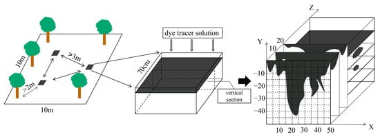
Figure 1.
Dye-tracing experiment.
The DC is defined as the ratio of the dye-stained area to the total area of the vertical profile [19].
where DC is dye coverage (%), D is the area of the stained region (cm2), and ND is the area of the unstained region (cm2).
The FD is used to reflect the complexity of the stained area in the soil profile. The higher the value is, the more complex the stained area is [27].
where FD is the fractal dimension, ε is the length of one side of the small cube, and N(ε) is the number of measured forms covered by this small cube.
2.6. IHC Characterization
The hydrological connectivity describes the transport of matter, energy, solutes, and information between the hydrological elements through water movement [32]. To compare and evaluate the hydrological connectivity of the two different tree species in the subtropics, the dye coverage (DC) and fractal dimension (FD) were used to construct the index of hydrologic connectivity (IHC) [27]. The dye coverage (DC) is a very important parameter in dye tracing experiments, and it reflects the degree of diffusion of water and solutes in the soil [33]. The fractal dimension (FD) of the dye image reflects the complexity of the wetting front of the soil water movement [34]. Even when the stained regions are identical, the degree of inconsistent fragmentation of the stained regions may lead to unequal IHC value. If the DC of the profile is the same, there is less hydrological connectivity between the stained regions when the FD is higher, so this region has more complex stained regional patches. In contrast, there are few complex staining patches at lower FD values, implying a high degree of hydrological connectivity in each stained region. The range of the IHC values is 0–1. The larger the IHC value is, the better the hydrological connectivity of this region is. When the IHC value is close to 1, the water exchange between the stained and unstained regions of the soil occurs more easily in this region. When the IHC value is close to 0, the forest has a weaker hydrological connectivity within the soils. The formula for calculating IHC is as follows [27].
where IHC is the index of the hydrological connectivity below the soil surface, DC is the dye coverage (%), FD is the fractal dimension, and n is the number of vertical soil staining profiles at a specific depth.
2.7. Back Propagation (BP) Neural Networks
In this study, the back propagation (BP) neural network has a simple structure and better performance, which has better applicability. Back propagation neural networks computed using the Neuralnet package in R were used to predict the relationships between the different factors (i.e., the parameters of root system architecture) affecting the IHC. The BP neural network contains an input layer, a hidden layer, and an output layer [35]. The structure of the BP neural network is shown in Figure 2. The number of nodes in the input layer is 6. In the model, the number of nodes in the first hidden layer is 8, and that in the second hidden layer is 8. The number of nodes in the output layer is 1. The generalized weight (GW) was calculated using the Neuralnet package in R to estimate the relative importance of the variables for the changes in IHC.
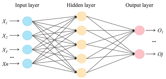
Figure 2.
The structure of the BP neural network.
The input and output data are normalized. The formula is as follows [27]:
where Xmin and Xmax are the minimum and maximum values of the input matrix and output vector quantity, respectively, and Xi is the real value of each vector quantity.
The input value of the BP neural network is expressed as . The implicit layer excitation function f selected in this study is:
The output of the hidden layer can be obtained as follows:
where is the connection weight between the input layer and the output layer, is the hidden layer threshold, f is the activation function of the hidden layer, is the input of the hidden layer node, and l is the number of nodes in the hidden layer.
The predicted output of the BP neural network can be obtained as follows:
where is the connection weight, is the output layer threshold.
The goodness of fit (R2) of the BP model, which reflects the difference between the predicted output and the expected output , are calculated as follows:
The generalized weight (GW) values were used to estimate the relative importance of the different factors of IHC [28]. The GW is calculated as follows:
2.8. Data Analysis
In this study, Pearson correlation coefficient analysis was performed using SPSS (Statistical Product Service Solutions) 27.0 software (SPSS Inc., Chicago, IL) to determine the correlation between each parameter of root system architecture. The analysis was also used to quantify the correlation between each parameter of root system architecture and the IHC in pine (SS) and bamboo (ZL) forests. The results were statistically significant at the 5% significance level, and the r value was obtained from the analysis [36]. The mean values of each parameter of root system architecture and the IHC of each soil depth were calculated in the 95% confidence interval (CI). The differences between each root parameter in the two sites were analyzed using independent samples T-test, and also for the difference in the IHC. Two-way ANOVA was used to compare the differences in the IHC value at different depths in the two sites.
The Origin 2021 software (OriginLab Corp., Northampton, MA) was considered to simulate the quantitative correlations between root system architecture and the IHC [37,38]. Based on the results of this study, the logarithm equation was considered to better characterize their correlations. Back propagation (BP) neural networks using the Neuralnet package in R 4.1.3 (R Foundation for Statistical Computing, Vienna, Austria) were used to predict the relative importance of the variables (i.e., the parameters of root system architecture) for the changes of the IHC on the basis of the values of general weight (GW) [27].
3. Results
3.1. Calculation of IHC within the Soils Using DC and FD
The results revealed that the change trends of the DC and FD were similar, that is, in the pine (SS) and bamboo (ZL) forests, both the DC and FD decreased with increasing soil depth (Figure 3), and the IHC value also decreased with increasing soil depth (Figure 4). The IHC value in the SS site decreased slowly at the surface soils (10–20 cm) and rapidly at the deeper depths (Figure 4). For the surface soil layer (0–10 cm), the IHC value was 0.467 (95%CI, 0.435 to 0.500) in the SS site and 0.483 (95%CI, 0.432 to 0.535) in the ZL site. For the 10–20 cm soil layer, the IHC value was 0.453 (95%CI, 0.439 to 0.467) in the SS site and 0.420 (95%CI, 0.331 to 0.509) in the ZL site. For the deeper soils (20–30 cm), the IHC value was 0.290 (95%CI, 0.162 to 0.418) in the SS site and 0.336 (95%CI, 0.160 to 0.511) in the ZL site. When the soil depth reached 30–40 cm, the IHC value was 0.146 (95%CI, 0.041 to 0.250) in the SS site and 0.198 (95%CI, 0.002 to 0.394) in the ZL site. In the 40–50 cm soil layer, the IHC value reached a minimum value of 0.045 (95%CI, −0.034 to 0.124) in the SS site and 0.109 (95%CI, −0.025 to 0.243) in the ZL site. There was no significant difference in the IHC values between pine (SS) and bamboo (ZL) forests (p > 0.05), but the IHC values at different depths both in the SS site and the ZL site showed a significant difference (p < 0.05).
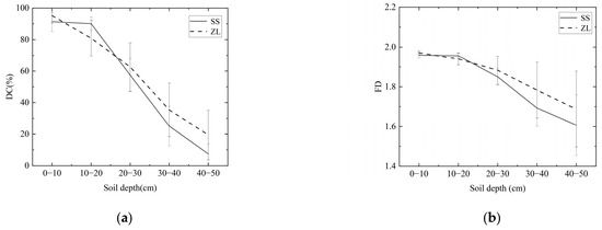
Figure 3.
Change trend of DC and FD with increasing soil depth in the two sites: (a) Change trend of DC with increasing soil depth; (b) Change trend of FD with increasing soil depth.
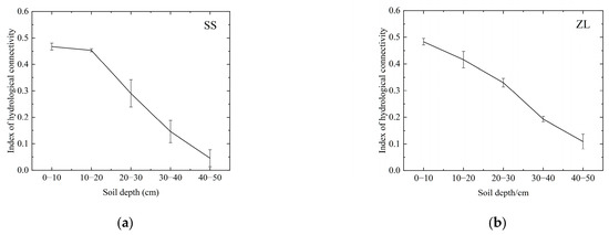
Figure 4.
Change trend of IHC with increasing soil depth in the two sites: (a) Change trend of the IHC values in the SS site with increasing soil depth; (b) Change trend of the IHC values in the ZL site with increasing soil depth.
3.2. Interaction between the Root System and IHC
The parameters of root system architecture decreased with increasing soil depth in the SS and ZL sites, and the parameters in the bamboo forest (ZL) were significantly higher than that in the pine forest (SS) (p < 0.05) (Table 3). It was found that root systems were rich at the soil surface. Top soil layers (0–20 cm) got the maximum root systems content. Taking the root length as an example, the value of the root length was 198.87 (95%CI, 103.85 to 275.89) cm/100 cm3 in the 0–10 cm soil layer in the SS site, but it was 699.28 (95%CI, 69.65 to 1328.90) cm/100 cm3 in the ZL site. In the 40–50 cm soil layer, the value of the root length was 25.84 (95%CI, 11.29 to 40.40) cm/100 cm3 in the SS site, and it was 93.40 (95%CI, −39.36 to 226.16) cm/100 cm3 in the ZL site. Each root parameter was fitted to the IHC values using the logarithm equation. The results obtained were shown in Figure 5 and Figure 6. The results showed that each parameter of root system architecture (the root length, projected root area, root surface area, root volume, and root biomass) was well fitted with the IHC, which showed that these parameters of root system architecture and the IHC were positively correlated. The IHC values increased with increasing parameters of root system architecture.
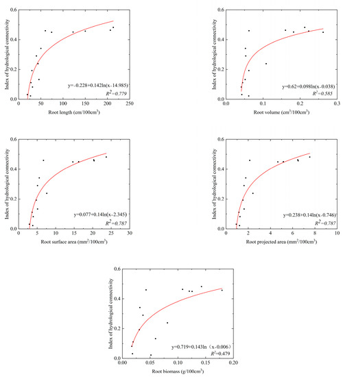
Figure 5.
The relationship between the parameters of roots system architecture and IHC in the SS site.
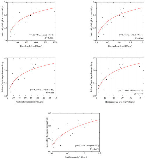
Figure 6.
The relationship between the parameters of roots system architecture and IHC in the ZL site.
Pearson correlation analysis was conducted between the IHC and the various parameters of root system architecture. The results were presented in Figure 7. The results showed that the parameters of root system architecture were significantly positively correlated with each other (p < 0.05). Among those parameters, the RL was more correlated with the IHC (r = 0.57, p < 0.01), whereas the relationship between the RAD and the IHC was not significantly different (r = 0.21, p > 0.05).
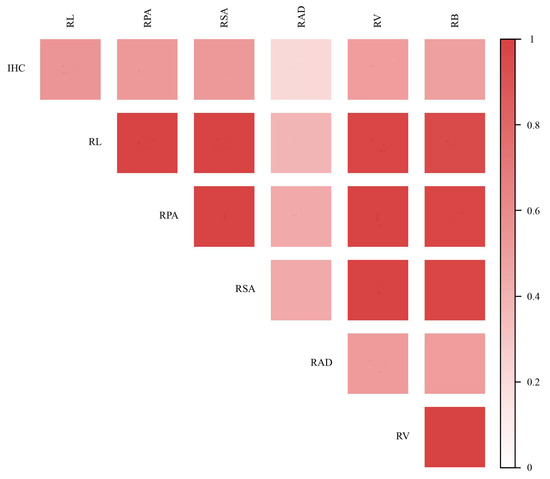
Figure 7.
Correlation between root parameters and IHC.
A BP neural network was used to predict the correlations between the different factors and the IHC. The BP neural network had an accurate simulation as the results were assessed (R2 = 0.76). The values of the GW in this study indicated that the RL was more sensitive and important to the IHC (Figure 8). The values of the GW for the RL were the highest among those parameters (Figure 8), which showed the highest importance of the RL for the changes in the IHC values. As the root length increased, the lengths of the channels within the soils formed by root production also increased, and the water circulation within the soils became easier [38]. In addition, the pore channels formed within the soils were expanded by the growth of the roots, which affected the water movement to a certain extent.
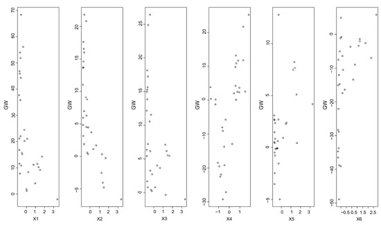
Figure 8.
The GW of different input factors’ contribution to the predicted output IHC (X1: root length; X2: root projected area; X3: root surface area; X4: root average diameter; X5: root volume; X6: root biomass).
As can be seen from Table 4, there was a significant correlation between the IHC and the root parameters with different root diameters, and the results showed that the very fine root systems (0 < D < 1 mm) [39] had a greater effect on the IHC both in the ZL and the SS sites (p < 0.01). From Table 4, it was found that root system architecture with root diameters D > 4 mm had no significant effects on the changes in the IHC. The correlation between the root parameters with different root diameters and the IHC was higher in the ZL sites than in the SS sites.
Table 4.
Analysis of the correlation between the IHC and root systems with different diameters.
4. Discussion
4.1. Hydrological Connectivity Evaluation Based on IHC
In this study, we used the IHC based on the DC and FD to characterize the strength of the hydrological connectivity below the soil surface in forest ecosystems. The results of this study demonstrate that the index of hydrological connectivity below the soil surface decreased with increasing soil depth, with the top layer of the soil exhibiting stronger connectivity. The result is consistent with the findings of Zhang et al. [19]. The transport and connectivity of the water within the soils are influenced by the physical properties of the soil and vegetation characteristics [40]. In general, forested areas have a more abundant litter and humus than other land cover types [41,42], and the litter at the soil surface can store precipitation during the initial stages of rainfall [43]. In addition, litter increases the roughness of the ground surface and increases the soil porosity [44], which can inhibit the occurrence of runoff and promote water infiltration to some extent [45,46]. The preferential channels generated by soil pores effectively promote the connectivity of water within the soils. The pine forest (SS) in this study had lower hydrological connectivity in the surface soil than the bamboo forest (ZL). This was probably due to the slower decomposition of coniferous forest litter [47], which did not have a positive effect on surface soil properties in the SS site compared with the litter in the ZL site [48]. Therefore, the IHC value at the soil surface region was higher in the bamboo forest (ZL) than in the pine forest (SS), which had better hydrological connectivity.
The soil’s physical properties, including the soil bulk density, soil porosity, and initial soil water content, affect the rate of water infiltration [49]. The lower initial water content of the surface soil increases the infiltration capacity of the water [50], which may explain the stronger hydrological connectivity of the surface soils in the pine forest (SS) compared to that in the bamboo forest (ZL). The total soil porosity is proportional to the rate of water infiltration, while the soil bulk density and initial water content are usually inversely proportional to the rate of water infiltration. Due to the high hydrological connectivity in the surface soil, the water infiltration into the top soil layer was more repaid. However, deeper soil layers with low water infiltration can lead to decreased hydrological connectivity. Furthermore, due to the lower root content in the deep soil, the soil capacity increases, the soil porosity decreases, and there are fewer preferential channels within the soils, so the connectivity of the water decreases. Finally, the amount of water that can infiltrate into the deeper layers of the soil is small and the IHC reaches a minimum value.
4.2. Root Systems and Hydrological Connectivity
The results of this study revealed that the parameters of root system architecture (the root length, projected root area, root surface area, root volume, and root biomass) and the IHC values were significantly positively correlated (Figure 7), which is consistent with the results of Zhang et al. [19] and Dai et al. [16]. Among them, the effect of the root length on the IHC values was the strongest. That is, among the various root parameters, the root length was the key factor influencing the water movement within the soils [51]. Many studies have shown that root characteristics, including root length, root diameter, and root biomass, influence the infiltration of soil water to some extent [52,53], enhancing the hydrological connectivity of the soil [54]. Roots can influence the hydrological response not only by changing the soil properties but also by forming preferential root channels. Complex root systems improve the soil porosity and create interconnected root channels, enhancing the infiltration capacity [55,56]. There is a richer network of root systems in the surface soil in pine and bamboo forests (Table 2), so it is possible for water to be transported more rapidly within the soils, leading to greater hydrological connectivity. When the root content was low and the characteristic parameters of the root systems were small, the IHC value was also low. The IHC increased as the values of the root parameters increased (Figure 5 and Figure 6). This is similar to the results of other studies because the root growth activity forms pore space and connects with the original pore space in the soil to form a pore network [12], which promotes water transport, and the root content of the soil in the surface layer is relatively higher, which has a significant effect on the promotion of water movement and improves the hydrological connectivity.
Our results show that the very fine root systems (0 < D < 1 mm) play an important role in the variation of the IHC. This is similar to the findings of Cui et al. [52]. Compared with thicker roots, fine roots can penetrate the soil better by using the pore space, and they have a stronger contact with the soil [57], which allows water to move along these small pores. Moreover, root diameter is a key factor in root decay and decomposition [52]. Thick roots decompose more slowly than fine roots, and the decay of thick roots is more dependent on climate, especially temperature [58]. The life cycle of fine roots is shorter, and they decay more quickly [59], with new roots replacing decaying roots [58]. The water connectivity is stronger in areas with fine root decay than in areas with thick roots [60]. However, Zhang et al. found that the thick root systems (3 < D < 5 mm) had a greater effect on the index of hydrological connectivity [19]. Dai et al. concluded that the thick roots (D > 5 mm) were positively correlated with the hydrological connectivity [16]. Having a thick root system with a high stiffness causes strong movement of soil particles, which increases the aggregated void space [57,61] and the decomposition of soil organic carbon [62]. In addition, the growth of thick roots leads to disruption of the soil aggregates and may form new pore spaces within the aggregates. A more developed root system forms a complex network of soil channels, resulting in better soil hydrological connectivity.
5. Conclusions
The results of this study show that in subtropical forest ecosystems, the index of the hydrological connectivity below the soil surface decreases with increasing soil depth. There was no significant difference in the IHC values between pine (SS) and bamboo (ZL) forests, but the IHC values at different depths both in the SS site and the ZL site showed a significant difference. The parameters of root system architecture (i.e., the root length, root projected area, root surface area, root volume, and root biomass) were rich in the surface soil (0–20 cm) and the parameters in the ZL site were significantly higher than that in the SS site. The root parameters were positively correlated with the changes in the IHC. Among those parameters, the root length had the largest positive influence on the hydrological connectivity. Furthermore, we found that the root system architecture with different root diameters had different degrees of influence on the index of hydrological connectivity. The very fine roots (0 < D < 1 mm) had the greatest effect on the hydrological connectivity.
Author Contributions
Conceptualization, Y.Z.; methodology, W.Z.; software, W.Z.; formal analysis, W.Z.; investigation, W.Z., L.W. and Z.T.; writing—original draft preparation, W.Z.; writing—review and editing, Y.Z.; funding acquisition, Y.Z. All authors have read and agreed to the published version of the manuscript.
Funding
This research was supported by the Postgraduate Research and Practice Innovation Program of Jiangsu Province (KYCX22_1123), the National Natural Science Foundation of China (41907007), and the Jiangsu Province Natural Science Foundation for Youth (BK20190747).
Data Availability Statement
Data are available from the authors on request.
Acknowledgments
We thank all staff of Xiashu scientific research base in Jiangsu Province, China for their assistance in our field experiments.
Conflicts of Interest
The authors declare no conflict of interest.
References
- Zhang, M.; Liu, N.; Harper, R.; Li, Q.; Liu, K.; Wei, X.; Ning, D.; Hou, Y.; Liu, S. A global review on hydrological responses to forest change across multiple spatial scales: Importance of scale, climate, forest type and hydrological regime. J. Hydrol. 2017, 546, 44–59. [Google Scholar] [CrossRef]
- Guo, G.; Li, X.; Zhu, X.; Xu, Y.; Dai, Q.; Zeng, G.; Lin, J. Effect of Forest Management Operations on Aggregate-Associated SOC Dynamics Using a 137Cs Tracing Method. Forests 2021, 12, 859. [Google Scholar] [CrossRef]
- Bruijnzeel, L. Hydrological functions of tropical forests: Not seeing the soil for the trees? Agric. Ecosyst. Environ. 2004, 104, 185–228. [Google Scholar] [CrossRef]
- Lexartza-Artza, I.; Wainwright, J. Hydrological connectivity: Linking concepts with practical implications. CATENA 2009, 79, 146–152. [Google Scholar] [CrossRef]
- Freeman, M.C.; Pringle, C.M.; Jackson, C.R. Hydrologic Connectivity and the Contribution of Stream Headwaters to Ecological Integrity at Regional Scales1. J. Am. Water Resour. Assoc. 2007, 43, 5–14. [Google Scholar] [CrossRef]
- Wainwright, J.; Turnbull, L.; Ibrahim, T.G.; Lexartza-Artza, I.; Thornton, S.F.; Brazier, R.E. Linking environmental régimes, space and time: Interpretations of structural and functional connectivity. Geomorphology 2011, 126, 387–404. [Google Scholar] [CrossRef]
- Li, Y.; Zhang, Q.; Cai, Y.; Tan, Z.; Wu, H.; Liu, X.; Yao, J. Hydrodynamic investigation of surface hydrological connectivity and its effects on the water quality of seasonal lakes: Insights from a complex floodplain setting (Poyang Lake, China). Sci. Total. Environ. 2019, 660, 245–259. [Google Scholar] [CrossRef]
- Nanda, A.; Sen, S.; McNamara, J.P. How spatiotemporal variation of soil moisture can explain hydrological connectivity of infiltration-excess dominated hillslope: Observations from lesser Himalayan landscape. J. Hydrol. 2019, 579, 124146. [Google Scholar] [CrossRef]
- Beven, K.; Germann, P. Macropores and water flow in soils revisited. Water Resour. Res. 2013, 49, 3071–3092. [Google Scholar] [CrossRef]
- Van Noordwijk, M.; Widianto; Heinen, M.; Hairiah, K. Old tree root channels in acid soils in the humid tropics: Important for crop root penetration, water infiltration and nitrogen management. Plant Soil 1991, 134, 423–430. [Google Scholar] [CrossRef]
- Zhang, Y.H.; Huang, C.Y.; Zhang, W.Q.; Chen, J.H.; Wang, L. The concept, approach, and future research of hydrological connectivity and its assessment at multiscales. Environ. Sci. Pollut. Res. 2021, 28, 52724–52743. [Google Scholar] [CrossRef]
- Alaoui, A.; Caduff, U.; Gerke, H.H.; Weingartner, R. Preferential Flow Effects on Infiltration and Runoff in Grassland and Forest Soils. Vadose Zone J. 2011, 10, 367–377. [Google Scholar] [CrossRef]
- Wilson, G.V.; Nieber, J.L.; Fox, G.; Dabney, S.M.; Ursic, M.; Rigby, J.R. Hydrologic connectivity and threshold behavior of hillslopes with fragipans and soil pipe networks. Hydrol. Process. 2017, 31, 2477–2496. [Google Scholar] [CrossRef]
- Wine, M.L.; Ochsner, T.E.; Sutradhar, A.; Pepin, R. Effects of eastern redcedar encroachment on soil hydraulic properties along Oklahoma’s grassland-forest ecotone. Hydrol. Process. 2012, 26, 1720–1728. [Google Scholar] [CrossRef]
- Hildebrandt, A. Root-Water Relations and Interactions in Mixed Forest Settings. For.-Water Interact. 2020, 240, 319–348. [Google Scholar] [CrossRef]
- Liyi, D.; Yinghu, Z.; Ying, L.; Lumeng, X.; Shiqiang, Z.; Zhenming, Z. Thick roots and less microaggregates improve hydrological connectivity. Chemosphere 2021, 266, 129008. [Google Scholar] [CrossRef] [PubMed]
- Ameli, A.A.; Creed, I.F. Quantifying hydrologic connectivity of wetlands to surface water systems. Hydrol. Earth Syst. Sci. 2017, 21, 1791–1808. [Google Scholar] [CrossRef]
- Shore, M.; Murphy, P.; Jordan, P.; Mellander, P.-E.; Kelly-Quinn, M.; Cushen, M.; Mechan, S.; Shine, O.; Melland, A. Evaluation of a surface hydrological connectivity index in agricultural catchments. Environ. Model. Softw. 2013, 47, 7–15. [Google Scholar] [CrossRef]
- Zhang, Y.H.; Jiang, J.; Zhang, J.C.; Zhang, Z.M.; Zhang, M.X. Effects of roots systems on hydrological connectivity below the soil surface in the Yellow River Delta wetland. Ecohydrology 2021, 15, e2393. [Google Scholar] [CrossRef]
- Liu, J.; Engel, B.A.; Zhang, G.; Wang, Y.; Wu, Y.; Zhang, M.; Zhang, Z. Hydrological connectivity: One of the driving factors of plant communities in the Yellow River Delta. Ecol. Indic. 2020, 112, 106150. [Google Scholar] [CrossRef]
- Saco, P.M.; Rodríguez, J.F.; Moreno-De Las Heras, M.; Keesstra, S.; Azadi, S.; Sandi, S.; Baartman, J.; Rodrigo-Comino, J.; Rossi, M.J. Using hydrological connectivity to detect transitions and degradation thresholds: Applications to dryland systems. CATENA 2020, 186, 104354. [Google Scholar] [CrossRef]
- Schwärzel, K.; Ebermann, S.; Schalling, N. Evidence of double-funneling effect of beech trees by visualization of flow pathways using dye tracer. J. Hydrol. 2012, 470–471, 184–192. [Google Scholar] [CrossRef]
- James, A.; Roulet, N.T. Investigating hydrologic connectivity and its association with threshold change in runoff response in a temperate forested watershed. Hydrol. Process. 2007, 21, 3391–3408. [Google Scholar] [CrossRef]
- Licznar, P.; Nearing, M. Artificial neural networks of soil erosion and runoff prediction at the plot scale. Catena 2003, 51, 89–114. [Google Scholar] [CrossRef]
- Naz, M.; Uyanik, S.; Yesilnacar, M.I.; Sahinkaya, E. Side-by-side comparison of horizontal subsurface flow and free water surface flow constructed wetlands and artificial neural network (ANN) modelling approach. Ecol. Eng. 2009, 35, 1255–1263. [Google Scholar] [CrossRef]
- Wen, H.; Bi, J.; Guo, D. Calculation of the thermal conductivities of fine-textured soils based on multiple linear regression and artificial neural networks. Eur. J. Soil Sci. 2020, 71, 568–579. [Google Scholar] [CrossRef]
- Zhang, Y.H.; Chen, J.H.; Zhang, J.C.; Zhang, Z.; Zhang, M. Novel indicator for assessing wetland degradation based on the index of hydrological connectivity and its correlation with the root-soil interface. Ecol. Indic. 2021, 133, 108392. [Google Scholar] [CrossRef]
- Li, J.; Wang, Y.K.; Guo, Z.; Li, J.B.; Tian, C.; Hua, D.W.; Shi, C.D.; Wang, H.Y.; Han, J.C.; Xu, Y. Effects of Conservation Tillage on Soil Physicochemical Properties and Crop Yield in an Arid Loess Plateau, China. Sci. Rep. 2020, 10, 4716. [Google Scholar] [CrossRef] [PubMed]
- Liu, Y.L.; Li, C.L.; Gao, M.X.; Zhang, M.; Zhao, G.X. Effect of different land-use patterns on the physical characteristics of the soil in the Yellow River delta region. Acta Ecol. Sin. 2015, 35, 5183–5190. [Google Scholar] [CrossRef][Green Version]
- Wang, M.B.; Zhang, Q. Issues in using the WinRHIZO system to determine physical characteristics of plant fine roots. Acta Ecol. Sin. 2009, 29, 136–138. [Google Scholar] [CrossRef]
- Ghodrati, M.; Jury, W.A. A Field Study Using Dyes to Characterize Preferential Flow of Water. Soil Sci. Soc. Am. J. 1990, 54, 1558–1563. [Google Scholar] [CrossRef]
- Bracken, L.J.; Wainwright, J.; Ali, G.A.; Tetzlaff, D.; Smith, M.W.; Reaney, S.M.; Roy, A.G. Concepts of hydrological connectivity: Research approaches, pathways and future agendas. Earth-Sci. Rev. 2013, 119, 17–34. [Google Scholar] [CrossRef]
- Gjettermann, B.; Nielsen, K.; Petersen, C.; Jensen, H.; Hansen, S. Preferential flow in sandy loam soils as affected by irrigation intensity. Soil Technol. 1997, 11, 139–152. [Google Scholar] [CrossRef]
- Ogawa, S.; Baveye, P.; Boast, C.W.; Parlange, J.Y.; Steenhuis, T. Surface fractal characteristics of preferential flow patterns in field soils: Evaluation and effect of image processing. Geoderma 1999, 88, 109–136. [Google Scholar] [CrossRef]
- Rumelhart, D.E.; Hinton, G.E.; Williams, R.J. Learning representations by back-propagating errors. Nature 1986, 323, 533–536. [Google Scholar] [CrossRef]
- Zhu, L.; Gong, H.; Dai, Z.; Xu, T.; Su, X. An integrated assessment of the impact of precipitation and groundwater on vegetation growth in arid and semiarid areas. Environ. Earth Sci. 2015, 74, 5009–5021. [Google Scholar] [CrossRef]
- Ebel, B.A.; Martin, D.A. Meta-analysis of field-saturated hydraulic conductivity recovery following wildland fire: Applications for hydrologic model parameterization and resilience assessment. Hydrol. Process. 2017, 31, 3682–3696. [Google Scholar] [CrossRef]
- Leslie, I.N.; Heinse, R.; Smith, A.M.S.; McDaniel, P.A. Root Decay and Fire Affect Soil Pipe Formation and Morphology in Forested Hillslopes with Restrictive Horizons. Soil Sci. Soc. Am. J. 2014, 78, 1448–1457. [Google Scholar] [CrossRef]
- Karimi, Z.; Abdi, E.; Deljouei, A.; Cislaghi, A.; Shirvany, A.; Schwarz, M.; Hales, T.C. Vegetation-induced soil stabilization in coastal area: An example from a natural mangrove forest. CATENA 2022, 216, 106410. [Google Scholar] [CrossRef]
- Leung, A.K.; Boldrin, D.; Liang, T.; Wu, Z.Y.; Kamchoom, V.; Bengough, A.G. Plant age effects on soil infiltration rate during early plant establishment. Géotechnique 2018, 68, 646–652. [Google Scholar] [CrossRef]
- Fung, T.K.; Richards, D.R.; Leong, R.A.T.; Ghosh, S.; Tan, C.W.J.; Drillet, Z.; Leong, K.L.; Edwards, P.J. Litter decomposition and infiltration capacities in soils of different tropical urban land covers. Urban Ecosyst. 2022, 25, 21–34. [Google Scholar] [CrossRef]
- Jordán, A.; Martínez-Zavala, L.; Bellinfante, N. Heterogeneity in soil hydrological response from different land cover types in southern Spain. CATENA 2008, 74, 137–143. [Google Scholar] [CrossRef]
- Dunkerley, D. Percolation through leaf litter: What happens during rainfall events of varying intensity? J. Hydrol. 2015, 525, 737–746. [Google Scholar] [CrossRef]
- Pavão, L.L.; Sanches, L.; Júnior, O.B.P.; Spolador, J. The influence of litter on soil hydro-physical characteristics in an area of Acuri palm in the Brazilian Pantanal. Ecohydrol. Hydrobiol. 2019, 19, 642–650. [Google Scholar] [CrossRef]
- Xia, L.; Song, X.; Fu, N.; Cui, S.; Li, L.; Li, H.; Li, Y. Effects of forest litter cover on hydrological response of hillslopes in the Loess Plateau of China. CATENA 2019, 181, 104076. [Google Scholar] [CrossRef]
- Zhou, Q.; Keith, D.; Zhou, X.; Cai, M.; Cui, X.; Wei, X.; Luo, Y. Comparing the Water-holding Characteristics of Broadleaved, Coniferous, and Mixed Forest Litter Layers in a Karst Region. Mt. Res. Dev. 2018, 38, 220–229. [Google Scholar] [CrossRef]
- Guo, P.; Jiang, H.; Yu, S.; Ma, Y.; Dou, R.; Song, X. Comparason of Litter Decomposition of Six Species of Coniferous and Broad-leaved Trees in Subtropical China. Chin. J. Appl. Environ. Biol. 2009, 2009, 655–659. [Google Scholar] [CrossRef]
- Osono, T. Leaf litter decomposition of 12 tree species in a subtropical forest in Japan. Ecol. Res. 2017, 32, 413–422. [Google Scholar] [CrossRef]
- Sun, D.; Yang, H.; Guan, D.; Yang, M.; Wu, J.; Yuan, F.; Jin, C.; Wang, A.; Zhang, Y. The effects of land use change on soil infiltration capacity in China: A meta-analysis. Sci. Total. Environ. 2018, 626, 1394–1401. [Google Scholar] [CrossRef] [PubMed]
- Alaoui, A. Modelling susceptibility of grassland soil to macropore flow. J. Hydrol. 2015, 525, 536–546. [Google Scholar] [CrossRef]
- Lange, B.; Lüescher, P.; Germann, P.F. Significance of tree roots for preferential infiltration in stagnic soils. Hydrol. Earth Syst. Sci. 2009, 13, 1809–1821. [Google Scholar] [CrossRef]
- Cui, Z.; Wu, G.L.; Huang, Z.; Liu, Y. Fine roots determine soil infiltration potential than soil water content in semi-arid grassland soils. J. Hydrol. 2019, 578, 124023. [Google Scholar] [CrossRef]
- Wu, G.L.; Yang, Z.; Cui, Z.; Liu, Y.; Fang, N.F.; Shi, Z.H. Mixed artificial grasslands with more roots improved mine soil infiltration capacity. J. Hydrol. 2016, 535, 54–60. [Google Scholar] [CrossRef]
- Cui, Y.; Zhang, Y.H.; Zhou, S.J.; Pan, Y.Y.; Wang, R.Q.; Li, Z.; Zhang, Z.M.; Zhang, M.X. Cracks and root channels promote both static and dynamic vertical hydrological connectivity in the Yellow River Delta. J. Clean. Prod. 2022, 367, 132972. [Google Scholar] [CrossRef]
- van Schaik, N.L.M.B. Spatial variability of infiltration patterns related to site characteristics in a semi-arid watershed. CATENA 2009, 78, 36–47. [Google Scholar] [CrossRef]
- Ghestem, M.; Sidle, R.C.; Stokes, A. The Influence of Plant Root Systems on Subsurface Flow: Implications for Slope Stability. Bioscience 2011, 61, 869–879. [Google Scholar] [CrossRef]
- Bodner, G.; Leitner, D.; Kaul, H.-P. Coarse and fine root plants affect pore size distributions differently. Plant Soil 2014, 380, 133–151. [Google Scholar] [CrossRef] [PubMed]
- Zhang, X.; Wang, W. The decomposition of fine and coarse roots: Their global patterns and controlling factors. Sci. Rep. 2015, 5, 9940. [Google Scholar] [CrossRef] [PubMed]
- Liu, Y.; Guo, L.; Huang, Z.; López-Vicente, M.; Wu, G.L. Root morphological characteristics and soil water infiltration capacity in semi-arid artificial grassland soils. Agric. Water Manag. 2020, 235, 106153. [Google Scholar] [CrossRef]
- Yavitt, J.B.; Harms, K.E.; Garcia, M.N.; Mirabello, M.J.; Wright, S.J. Soil fertility and fine root dynamics in response to 4 years of nutrient (N, P, K) fertilization in a lowland tropical moist forest, Panama. Austral Ecol. 2011, 36, 433–445. [Google Scholar] [CrossRef]
- Cui, L.L.; Li, X.; Lin, J.; Guo, G.; Zhang, X.; Zeng, G.R. The mineralization and sequestration of soil organic carbon in relation to gully erosion. CATENA 2022, 214, 106218. [Google Scholar] [CrossRef]
- Guan, X.; Jiang, J.; Jing, X.; Feng, W.T.; Luo, Z.K.; Wang, Y.G.; Xu, X.; Luo, Y.Q. Optimizing duration of incubation experiments for understanding soil carbon decomposition. GEODERMA 2022, 428, 116225. [Google Scholar] [CrossRef]


Publisher’s Note: MDPI stays neutral with regard to jurisdictional claims in published maps and institutional affiliations. |
© 2022 by the authors. Licensee MDPI, Basel, Switzerland. This article is an open access article distributed under the terms and conditions of the Creative Commons Attribution (CC BY) license (https://creativecommons.org/licenses/by/4.0/).