Using Advanced Machine-Learning Algorithms to Estimate the Site Index of Masson Pine Plantations

Abstract

The rapid development of non-parametric machine learning methods, such as random forest (RF), extreme gradient boosting (XGBoost), and the light gradient boosting machine (LightGBM), provide new methods to predict the site index (SI). However, few studies used these methods for SI modeling of Masson pine, and there is a lack of comparison of model performances. The purpose of this study was to compare the performance of different modeling approaches and the variability between models with different variables. We used 84 samples from the Guangxi Tropical Forestry Experimental Centre. Five-fold cross-validation was used and linear regression models were established to assess the relationship between the dominant height of the stand and different types of variables. The optimal model was used to predict the SI. The results show that the LightGBM model had the highest accuracy. The root mean square error (RMSE) was 3.4055 m, the relative RMSE (RMSE%) was 20.95, the mean absolute error (MAE) was 2.4189 m, and the coefficient of determination (R²) was 0.5685. The model with climatic and soil chemical variables had an RMSE of 2.7507 m, an RMSE% of 17.18, an MAE of 2.0630 m, and an R² of 0.6720. The soil physicochemical properties were the most important factors affecting the SI, whereas the ability of the climatic factors to explain the variability in the SI in a given range was relatively low. The results indicate that the LightGBM is an excellent SI estimation method. It has higher efficiency and prediction accuracy than the other methods, and it considers the key factors determining site productivity. Adding climate and soil chemical variables to the model improves the prediction accuracy of the SI and the ability to evaluate site productivity. The proposed Masson pine SI model explains 67.2% of the SI variability. The model is suitable for the scientific management of unevenly aged Masson pine plantations.

1. Introduction

Masson pine (Pinus massoniana Lamb.) is a light-loving and deep-rooted tree species. It has strong adaptability and tolerance to arid and barren soil [1,2]. Masson pine is the most widely distributed, resourceful, and versatile coniferous species in subtropical China and has great economic and ecological value. In the Guangxi Zhuang Autonomous Region, China, Masson pine is a major timber and silvicultural species used for afforestation of difficult sites because of its high adaptability [3]. It is also used to produce essential oils [4]; thus, it is crucial for local development. Therefore, the appropriate management of Guangxi Masson pine plantations is critical to ensuring local scientific development.

Site quality is the productive potential of land with an established forest or other vegetation type. It is an important tool for assessing the influence of the environment on forest productivity [5,6]. Site quality assessment provides an accurate and timely assessment of stand productivity and is a prerequisite for scientific silviculture and subsequent management [7,8,9]. The site index (SI) is the average height of the dominant trees at the baseline age. It has been widely used to evaluate stand quality [8,10,11]. This indicator is correlated with productivity [12,13], and stand density has a negligible effect on the height of the dominant tree species [14,15,16]. More importantly, the SI integrates the most important factors affecting tree growth, including topography, soil characteristics, and climate [17].

Early SI prediction methods have primarily focused on growth models, which have a number of drawbacks, i.e., low accuracy, a small number of variables, low robustness, and the tendency to fall into local minima [18,19]. Some authors have improved the accuracy of model estimation by adding key variables [20,21,22]; however, the improvement is not very significant.

Due to the limitations of growth models, many traditional regression modeling approaches with varying degrees of complexity have been used to predict the SI of various forests, such as multiple linear regression [23,24,25,26,27,28,29,30,31,32,33,34,35,36], partial least squares, lasso regression, and stepwise regression [37]. Due to the rapid development of artificial intelligence, several sophisticated machine-learning methods have also been used to model the SI, including random forests (RF) [38,39], boosted regression trees (BRTs) [40,41], support vector machines (SVMs) [42], artificial neural networks (ANNs) [40,41], generalized additive models (GAMs) [40,41,43], Cubist [44], and multivariate adaptive regression splines (MARS) [37]. In contrast to traditional statistical models, machine-learning methods can detect complex, nonlinear interactions between predictor and response variables without requiring statistical assumptions and predetermined mathematical equations [45]. It should be noted that RF and BRTs can quantify the relative importance of variables with relatively high accuracy [40,44]. RF performs better than ANNs and SVMs for regression problems [46,47].

Advanced machine learning methods, such as extreme gradient boosting (XGBoost) and the light gradient boosting machine (LightGBM), have recently emerged as powerful algorithms based on BRTs. XGBoost and LightGBM have provided accuracies exceeding 80% in engineering [48], transportation [48,49], and gene recognition [50,51]. They also have been successfully used in biology and ecology for carbon measurements [52,53], forest biomass estimation [54], and species distribution [55,56]. These methods have recently been applied to assess stand productivity, particularly in studies comparing non-parametric and parametric models [57,58,59]. RF and XGBoost have been used to establish non-parametric SI models and achieved good prediction results [57,58]. However, the LightGBM has not been used to predict SIs.

Climate factors and soil conditions substantially influence stand productivity and site quality because they affect water, nutrients, temperature, and other conditions necessary for the growth of forest trees and their functions. Temperature and precipitation, the most prevalent climatic factors, significantly impact SIs [23,60,61]. Soil physical properties, such as soil type, layer thickness, and moisture content were initially used to predict SIs [62,63,64]. Similarly, soil chemical properties have also been widely used for SI estimation [60,65].

Therefore, the purpose of this study was to use linear regression and machine-learning algorithms to predict an SI and its range using multiple factors. Our objectives were to (1) compare and evaluate the performance of linear regression, RF, XGBoost, and LightGBM for SI modeling, (2) determine the variable importance, (3) compare machine-learning models and classical SI models to determine the advantages and disadvantages of incorporating climatic and soil chemical variables, and (4) use the optimal model to predict the SI of unevenly aged Masson pine plantations.

2. Materials and Methods

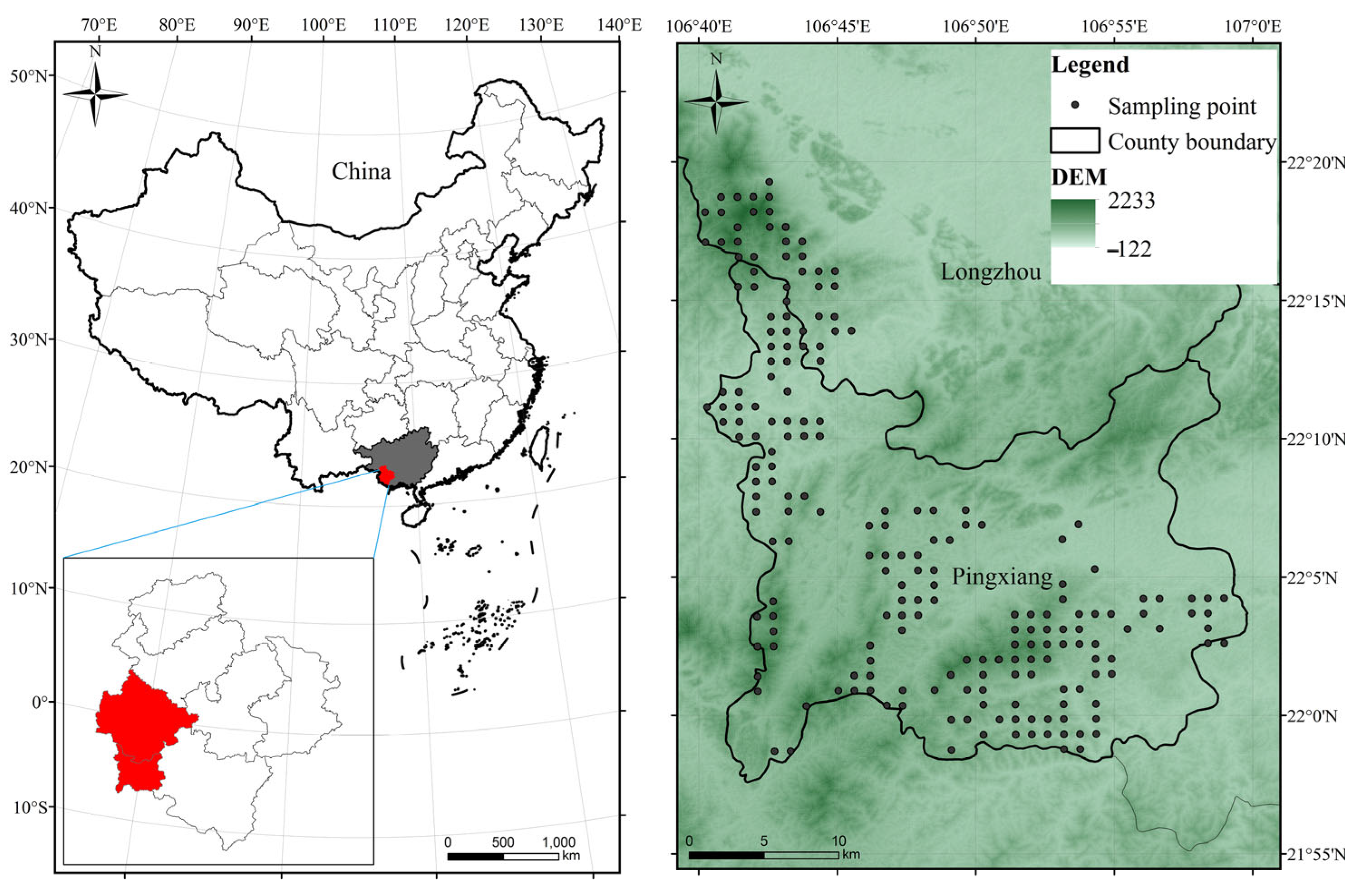
2.1. Study Area

The study area was the Tropical Forestry Experimental Centre of the Chinese Academy of Forestry Science (hereinafter referred to as TFC (21°57′47″–22°19′27″ N, 106°39′50″–106°59′30″ E) in Pingxiang and Longzhou City, Guangxi Zhuang Autonomous Region. The area has a semi-humid monsoon climate and is located in the southern subtropical zone, with abundant sunshine and rainfall. The annual precipitation is 1062–1772 mm, annual evaporation is 1261–1388 mm, and the annual average temperature of 21–23 °C, with a maximum temperature of 40.3 °C and a minimum temperature of −1.5 °C. The terrain is predominantly hilly, with an average altitude of 500–800 m, and the dominant soil types are brick red loam and red soil.

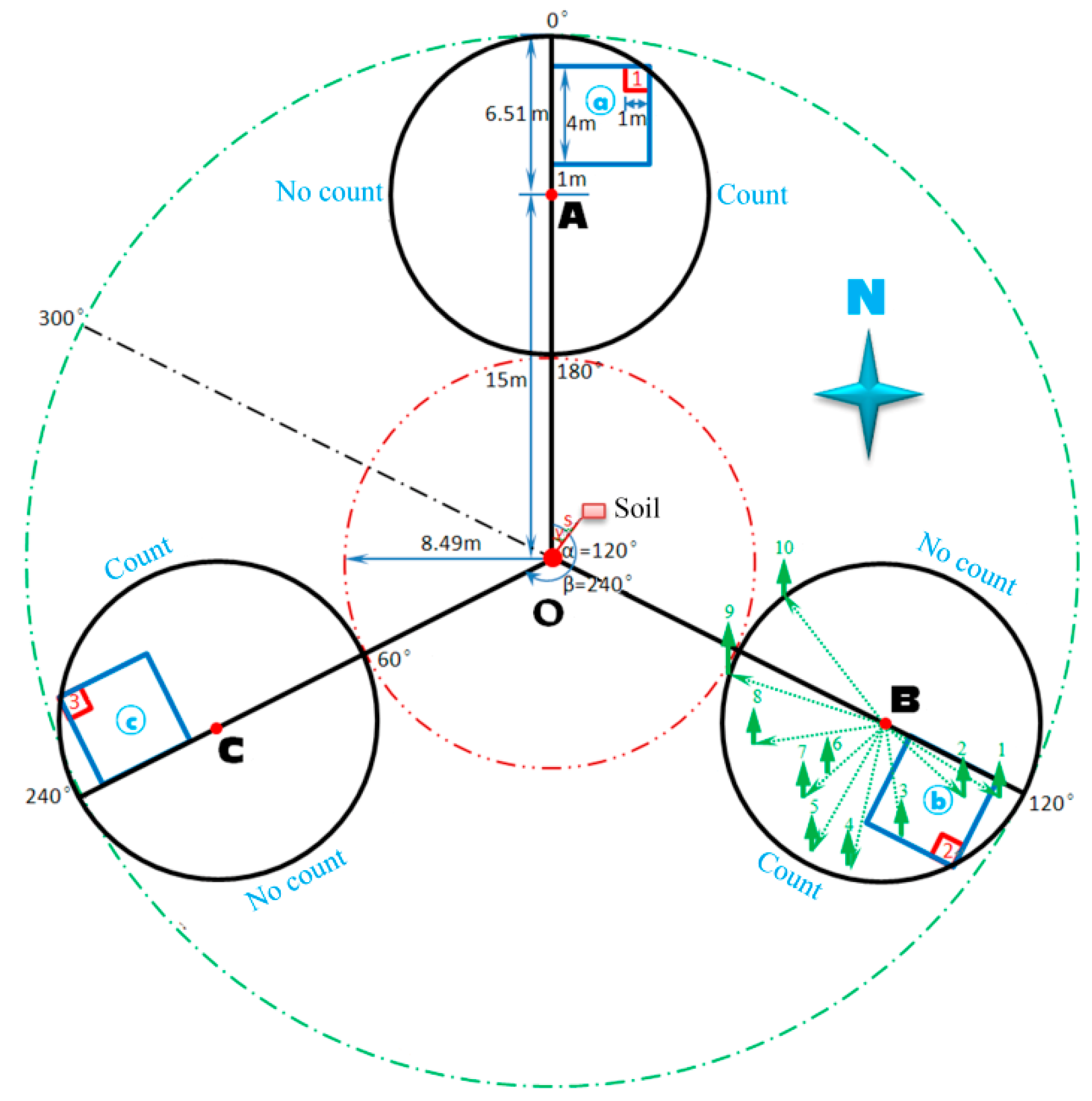
2.2. Plot Layout and Data Collection

In this study, field measurement data were obtained with traditional measuring instruments in the forest inventory such as the diameter tape for DBH measurement and Ultrasonic Height Gauge VLP-5 for tree height measurement. We used 238 sample plots (Figure 1) established in 2015 at the TFC. Each circular plot had an area of 400 m² (Figure 2) and contained three circular subsamples (A, B, C) with a radius of R = 6.51 m. Within these subsamples, 4 m × 4 m plots were used to measure young shrub (a, b, c), and 1 m × 1 m plots were used to measure young herbaceous plants (1, 2, 3). At the center of the sample plots (O), stand factors were recorded, such as elevation, slope, and slope orientation. In the three circular sample plots, the tree species, diameter at breast height, tree height, depression, origin, and stem quality of all trees with a diameter at breast height ≥5 cm were recorded. The average height, number, and cover of shrubs were recorded in the young shrub layer plots, and the number of seedlings, height, and cover of herbaceous species were recorded in the young herbaceous sample plots. Soil samples from layers O, A, and B were obtained within 8.49 m² near the center of each tree sample plot. We carefully removed the litter layer and took three soil samples from each layer with a ring knife and mixed them together in the sampling bags. We selected 84 plantation sample plots from the 238 systematically sampled plots. Masson pine was the dominant species. The summary statistics of the plot data are listed in

Table 1. Summary statistics of plot data stand investigation factors.

Variable	Description	Minimum	Maximum	Mean	Sd
Age (a)	Average stand age	3.0	38.0	19.4	8.6
N (trees∙hm−2)	Number of trees per hectare	250	1750	827	340
H (m)	Average stand height	4.1	22.2	10.8	3.2
Hd (m)	Dominant height of stand	5.5	29.1	15.2	4.7

.

2.3. Data and Preliminary Analysis

2.3.1. Dominant Height of the Stand

The data for the SI require time-resolved data for Masson pine, whereas the measurements in this study were stand age and tree height. Therefore, we predicted the SI using a dominant-height-based SI model, which reflects the relationship between the dominant height of a stand and the stand age. The arithmetic mean of the heights of the four tallest trees per 400 m² was used to calculate the dominant height of the stand (Table 1); this approach has been used in similar studies in Guangxi [19].

2.3.2. Soil Data

The site factors required for the evaluation included three categories: geographical, climatic, and soil factors. Geographical factors (altitude, slope, slope aspect, and slope position) were measured in the field survey. Soil factors included the physicochemical properties of the soil. The physical factors, such as soil type, soil layer thickness, and humus thickness, were obtained from field surveys and measurements, whereas the chemical factors were obtained from analyzing the soil samples collected in the field. The collected samples were taken to the laboratory and allowed to air dry before being weighed and ground. The milled soil samples were placed in soil sieves of 0.149 mm and 2 mm pore size, and the sieved samples were analyzed. The soil chemical indicators measured in this study were soil pH and elemental content, i.e., total nitrogen, total phosphorus, total potassium, hydrolyzed nitrogen, effective phosphorus, fast-acting potassium, and total organic carbon content.

2.3.3. Climate Data

The climate data were provided by ClimateAP, an application for dynamic surface temperature and precipitation calculations applied to historical and future climate data in the Asia–Pacific region [66,67,68]. Several climate variables, such as precipitation, temperature [60], air humidity [69], air CO₂ content [61], and solar radiation [57], have been used to study the effects of climate change on forests. We chose the mean annual temperature (MAT) and mean annual precipitation (MAP) [70,71,72,73] as the climatic variables for this study.

Table A1. Description of quantitative variables.

Variable Type	Number	Variable	Variable Definition
Geographical variables	4	Altitude	Vertical distance above sea level
		Aspect	Orientation of the slope
		Slope	Slope value
		Position	Slope position
Soil physical variables	3	ST	Soil type
		St	Soil thickness
		Ht	Soil humus layer thickness
Soil chemical variables	8	PH	Soil pH value
		TOC	Total soil organic carbon content
		TN	Total soil nitrogen content
		TP	Total soil phosphorus content
		TK	Total soil potassium content
		N	Soil available nitrogen content
		P	Soil available phosphorus content
		K	Soil available potassium content
Climate variables	2	MAT	Mean annual temperature
		MAP	Mean annual precipitation
Forest variables	1	Age	Average stand age

provides a description of all categories of quantitative variables.

2.4. Quantification of Category Characteristics

Since most regression models cannot use qualitative categorical variables, the categorical variables must be converted into numerical variables. The qualitative factors in this study were soil type, slope aspect, and slope position, and the categories of the three variables were assigned numbers from 1 to 5.

Table 2. Conversion of categorical variables into numerical variables (soil type, aspect, slope position).

Feature	Ⅰ	Ⅱ	Ⅲ	Ⅳ	Ⅴ
Soil type	reddish yellow	brick red	red	crimson	purple
Aspect	no slope	shady slope	semi-shady slope	semi-sunny slope	sunny slope
Slope position	flat slope	gentle slope	ramp	steep slope	dangerous slope

shows the results.

2.5. Modelling Methods

All modeling in this study was carried out with Python version 3.7.6. We used linear regression and three machine learning algorithms, i.e., RF, XGBoost, and LightGBM. We designed four data scenarios: (1) basic data (geographic factors and soil physical properties), (2) basic data with climate data, (3) basic data with soil data, and (4) all data. The data with added climatic and soil chemical properties and the basic data were randomly divided into training and test sets with a ratio of 7:3, respectively, and the training set was divided into sub-training and sub-validation sets using 5-fold cross-validation. The choice of hyperparameters determines the upper limit of the accuracy of machine-learning models. The machine-learning algorithm was based on cross-validation with a grid search method to obtain the optimal combination of hyperparameters and improve the performance and prediction accuracy of the model. The library used for the grid search was scikit-learn version 0.24.2.

Table A2. Hyperparametric variables of machine learning algorithm models (RF, XGBoost, LightGBM) and its grid search range.

Variable Name	Variable Definition	Method
		RF	XGBoost	LightGBM
N_estimators	Number of trees	500–1500	500–1500	500–1500
Max_depth	Maximum depth of the tree	3–15	3–15	−1–15
Min_samples_split	Minimum sample size required to split nodes	1–4	—	—
Min_samples_leaf	Minimum value of samples on leaf node	1,2	—	—
Min_child_weight	Minimum sample weight sum of leaf nodes	—	1–6	1–6
Gamma (min_gain_to_split)	Decreasing value of minimum loss function required for node splitting	—	0–1	0–1
Num_leaves	Number of leaf nodes of the tree	—	5–100	5–100
Subsample	Proportion of tree random sampling	—	0.6–1	0.6–1
Colsample_bytree	Feature sampling scale	—	0.1–1	0.1–1
Learning_rate	Tree model learning rate	—	0.01–0.2	0.01–0.2
Lambda_l1	L1 regularization term	—	10−5–1	10−5–1
Lambda_l2	L2 regularization term	—	10−5–1	10−5–1

shows the combinations of hyperparameter variables for each model and their grid search ranges.

2.5.1. Multiple Linear Regression

The model in Equation (1) is a multivariate linear model. The objective of least squares fitting is to determine the set of parameters that minimize the objective function. An estimate of the parameter vector can be obtained by finding the derivative of the function with respect to each parameter [22]. The main steps of the linear regression model are variable identification, parameter estimation, and precision testing. Since the objective of his study is to assess the model’s predictive ability, the multicollinearity between variables is not considered.

$$y={\beta }_0+{\beta }_1{x}_1+{\beta }_2{x}_2+\dots +{\beta }_m{x}_m$$

(1)

where x_i denotes the observations of the independent variable, y_i denotes the observations of the dependent variable, y is the vector of observations of the dependent variable, and β is the vector of the model parameters.

2.5.2. Random Forest

The RF algorithm was proposed by Leo Breiman in 2001. It is a machine-learning algorithm based on decision trees [74] with a bagging algorithm and an ensemble learning method. An RF consists of multiple uncorrelated regression trees; the final output of the model is based on all decision trees in the forest [40,41]. The model is constructed by randomly selecting m sample points from the training sample set S to obtain a new S1...Sn sub-training set that is used to train the regression tree (CART). During execution, k features are selected randomly, and the optimal cut point is selected at each node before performing left and right subtree partitioning. Multiple CARTs are obtained, and the final prediction of each regression tree is the mean of the leaf nodes at that sample point. The final prediction of the RF is the mean of the predictions of all regression trees.

2.5.3. Extreme Gradient Boosting

The XGBoost algorithm was developed by Tianqi Chen in 2016 and has proven to be a very reliable, efficient, and accurate regression method [75]. Boosting is also an ensemble learning method, but the classifiers are not equally weighted, unlike in the bagging algorithm. Boosting is performed using multiple simple weak classifiers. Each step produces a weak predictive model, which is then weighted and incorporated into the final model to construct a strong classifier with high accuracy that can be used for regression and classification problems [76,77]. If each step of the weak predictive model generation is based on the direction of the loss function’s gradient, it is called gradient boosting. The objective of approximating the local minimum of the loss function is achieved after several steps. XGBoost is based on gradient boosting decision trees (GBDTs). Weak models are added sequentially to a tree model to create a strong model in a region where the gradient descent algorithm generates the model’s objective function to predict the outcome. XGBoost is superior to GBDT in terms of model complexity, learning rate, overfitting prevention, missing value handling, and parallel computing.

2.5.4. Light Gradient Boosting Machine

The LightGBM algorithm is a boosting algorithm developed by the Microsoft DMTK team in 2017. It uses a tree algorithm [78]. This algorithm has few reading resources and is mainly used in online machine-learning competitions because of its good performance. It differs from other tree-based algorithms in that it grows the tree in a leafy manner (hierarchically) rather than horizontally. LightGM uses less memory than XGBoost. Thus, a single machine can operate at high speed, and the efficiency is improved when multiple machines are run in parallel, reducing the hardware requirements for data analysis. LightGBM provides a robust baseline and high efficiency without requiring feature selection methods [56]. It has not been used for assessing forest site productivity.

2.6. Variable Importance

This study used the relative importance of the variables to describe the degree of influence of the characteristic variables on the dominant height of the stand. The magnitude of the parameters of each variable reflects the variable importance in a linear model. The variable importance of the machine learning algorithm models was determined using the feature importance functions in RF, XGBoost, and LightGBM. A comprehensive analysis was carried out using feature visualization and by ranking the variables according to their importance.

2.7. Model Evaluation

The coefficient of determination (R²), root mean square error (RMSE), relative root mean square error (RMSE%), and mean absolute error (MAE) are commonly used evaluation metrics for regression problems. Thus, they were chosen for the accuracy evaluation of the model based on cross-validation. Min-max normalization of the data to a range of 0 to 1 was performed to improve the convergence speed and accuracy of the linear regression models. RF, XGBoost, and LightGBM models are based on decision trees; thus, they require no normalization. The min-max normalization is defined in Equation (2), and the evaluation metrics are defined in Equations (3)–(6).

$$x_j=\frac{x_i-x_{\min }}{x_{\max }-x_{\min }}$$

(2)

$$R^2=1-{\displaystyle \sum }_{i=1}^n\frac{{\left(Y_i-{\widehat{Y}}_i\right)}^2}{{\left(Y_i-\overline{Y}\right)}^2}$$

(3)

$$RMSE=\sqrt{\frac{{\displaystyle {\displaystyle \sum }_{i=1}^n}{\left(Y_i-{\widehat{Y}}_i\right)}^2}{n}}$$

(4)

$$RMSE\%=\frac{RMSE}{\overline{Y}}\ast 100$$

(5)

$$MAE=\frac{1}{n}{\displaystyle \sum }_{i=1}^n\left|Y_i-{\widehat{Y}}_i\right|$$

(6)

where x_i is the value of the variable before normalization, x_j is the normalized value of the variable, x_min is the minimum value of the sample data, x_max is the maximum value of the sample data, n is the number of observed samples, Ȳ is the mean of all samples of the dominant height, Y_i is the observed value of the dominant height of the ith sample, and Ŷ_i is the predicted value of the dominant height of the ith sample.

2.8. SI Prediction

The SI is the height of the dominant trees of the stand at the baseline age, which is the age at which stand growth has stabilized [13,14]. Most international scholars use the age of the tree when it reaches a height of 1.37 m or 30 a as the baseline age for model establishment. Most Chinese scholars have used 20 a or 30 a as the baseline age for stand growth models [7,11,19]. In this study, a baseline age of 30 a was used by referring to previous studies and considering the conditions in the study area and the growth characteristics of the Masson pine plantation. The model with the best prediction results was used to predict the SI in the study area based on the baseline age of the Masson pine plantation.

3. Results

3.1. Modeling Results

3.1.1. Machine-Learning Model Hyperparameters

The hyperparameters were tuned according to the hyperparameter combinations using a grid search method. Since the scenarios had different variables, the same modeling method required separate hyperparameter tuning depending on the type of variables in the model.

Table 3. Optimal hyperparameters for the machine learning models (RF, XGBoost, LightGBM) with different variable types.

Model	Optimal Hyperparameter Value
Models without climate and soil chemical variables
RF	N_estimators = 1000, Max_depth = 8, Min_samples_split = 2, Min_samples_leaf = 2
XGBoost	N_estimators = 950, Max_depth = 5, Min_child_weight = 3, Gamma = 0.1, Num_leaves = 10, Subsample = 0.4, Colsample_bytree = 0.4, Learning rate = 0.01, Lambda_l1 = 0.01, Lambda_l2 = 0.2
LightGBM	N_estimators = 1000, Max_depth= −1, Min_child_weight = 3, Gamma = 0.2, Num_leaves = 10, Subsample = 0.5, Colsample_bytree = 0.6, Learning_rate = 0.01, Lambda_l1 = 0.05, Lambda_l2 = 0.5
Models with climate variables
RF	N_estimators = 950, Max_depth = 10, Min_samples_split = 2, Min_samples_leaf = 2
XGBoost	N_estimators = 850, Max_depth = 5, Min_child_weight = 3, Gamma = 0.1, Num_leaves = 12, Subsample = 0.6, Colsample_bytree = 0.6, Learning_rate = 0.01, Lambda_l1 = 0.011, Lambda_l2 = 0.1
LightGBM	N_estimators = 1050, Max_depth = 1, Min_child_weight = 5, Gamma = 0.5, Num_leaves = 9, Subsample = 0.5, Colsample_bytree = 0.8, Learning_rate = 0.01, Lambda_l1 = 0.1, Lambda_l2 = 1.0
Models with soil chemical variables
RF	N_estimators = 1000, Max_depth = 10, Min_samples_split = 4, Min_samples_leaf = 2
XGBoost	N_estimators = 950, Max_depth = 5, Min_child_weight = 5, Gamma = 0.01, Num_leaves = 12, Subsample = 0.6, Colsample_bytree = 1.0, Learning_rate = 0.01, Lambda_l1 = 0.01, Lambda_l2 = 0.01
LightGBM	N_estimators = 1050, Max_depth = 3, Min_child_weight = 8, Gamma = 0.8, Num_leaves = 5, Subsample = 0.6, Colsample_bytree = 0.8, Learning_rate = 0.01, Lambda_l1 = 0.01, Lambda_l2 = 0.8
Models with climate and soil chemical variables
RF	N_estimators = 750, Max_depth = 15, Min_samples_split = 4, Min_samples_leaf = 2
XGBoost	N_estimators = 1050, Max_depth = 5, Min_child_weight = 5, Gamma = 0.0, Num_leaves = 15, Subsample = 0.6, Colsample_bytree = 1.0, Learning_rate = 0.02, Lambda_l1 = 0.001, Lambda_l2 = 0.01
LightGBM	N_estimators = 1200, Max_depth = 3, Min_child_weight = 11, Gamma = 0.9, Num_leaves = 5, Subsample = 0.6, Colsample_bytree = 0.9, Learning_rate = 0.01, Lambda_l1 = 0.001, Lambda_l2 = 0.9

list the optimal hyperparameter combinations for the machine-learning algorithms with different variable types. There are four hyperparameters in RF. In addition to the usual number of trees and maximum tree depth, the minimum number of samples required to split a node and the minimum value of the samples at a node were also added for more comprehensive tuning. XGBoost and LightGBM each have 10 hyperparameters with the same meaning, and the optimal combination of parameters for the two models is significantly different.

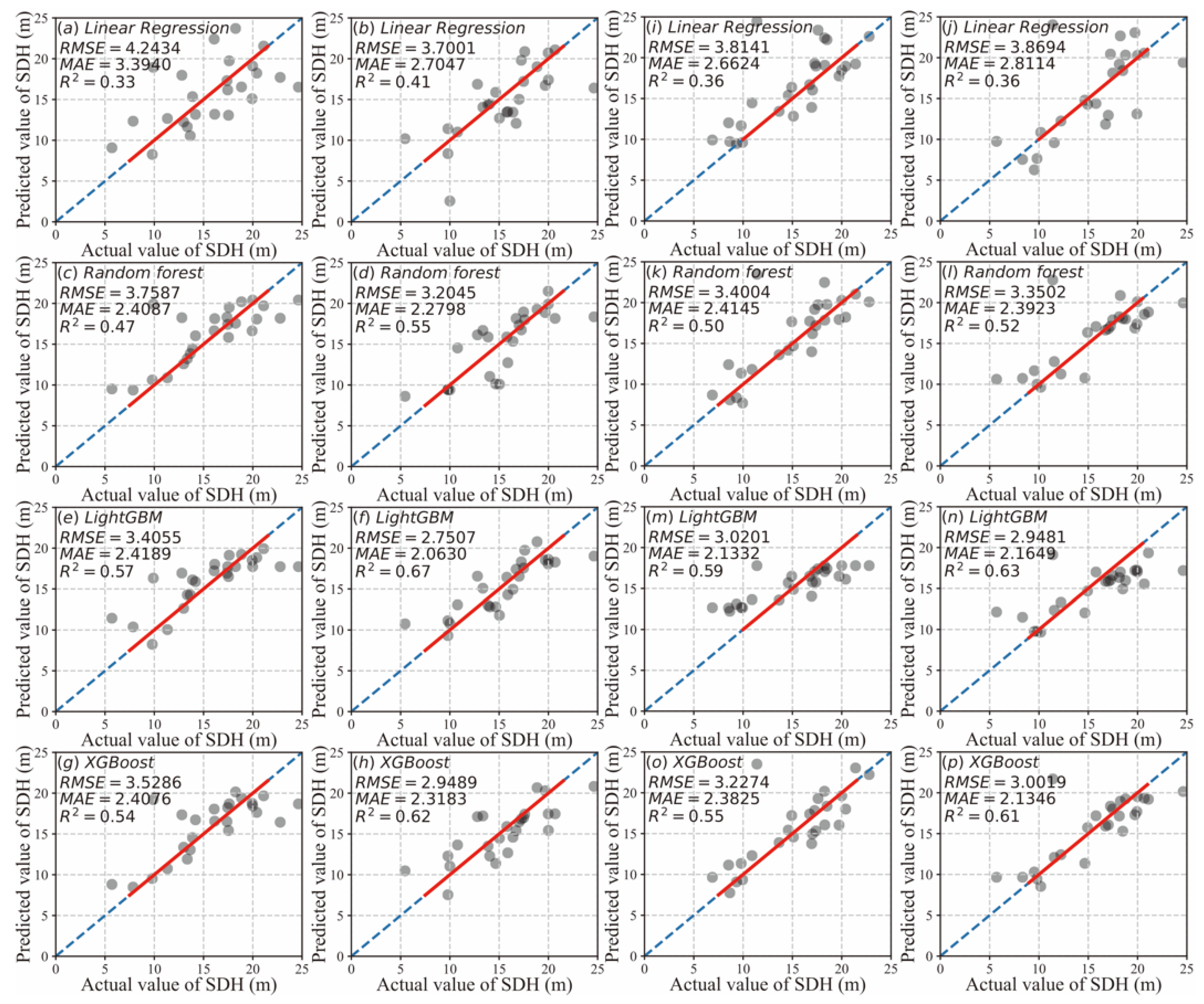
3.1.2. Model Comparison

Four parametric multiple linear regression models and twelve non-parametric machine-learning models were developed.

Table 4. The prediction accuracy of the SDH for different variable types obtained from parametric (linear regression) and non-parametric methods (RF, XGBoost, and LightGBM).

Variables	Model	RMSE	RMSE%	MAE	R2
		m	%	m
Without climate and soil chemical variables	Linear regression	4.2434	26.11	3.3940	0.3301
	RF	3.7587	23.12	2.4087	0.4744
	XGBoost	3.5286	21.71	2.4076	0.5368
	LightGBM	3.4055	20.95	2.4189	0.5685
With climate variables	Linear regression	3.8141	25.56	2.6624	0.3696
	RF	3.4004	22.79	2.4145	0.4989
	XGBoost	3.2274	21.63	2.3825	0.5486
	LightGBM	3.0201	19.66	2.1332	0.5951
With soil chemical variables	Linear regression	3.8694	26.61	2.8114	0.3564
	RF	3.3502	22.64	2.3923	0.5199
	XGBoost	3.0019	18.98	2.1346	0.6132
	LightGBM	2.9481	18.32	2.1649	0.6255
With climate and soil chemical variables	Linear regression	3.7001	23.10	2.7047	0.4065
	RF	3.2045	20.01	2.2798	0.5549
	XGBoost	2.9489	18.41	2.3183	0.6230
	LightGBM	2.7507	17.18	2.0630	0.6720

lists the prediction accuracy of the SDH for different variable types. The machine-learning models outperformed the linear regression models in the basic data scenarios (without climate and soil chemical variables). The models did not perform as well for these two types of data scenarios as for the scenarios with all data. The LightGBM model performed best for the basic scenario (RMSE = 3.4055, RMSE% = 20.95, MAE = 2.4189, and R² = 0.5685) and for the scenario with climate and soil chemical variables (RMSE = 2.7507, RMSE% = 17.18, MAE = 2.0630, and R² = 0.6720). It is worth mentioning that XGBoost and LightGBM outperformed RF according to all evaluation metrics, and the difference in the values of the evaluation metrics was small. Thus, LightGBM proved to be the most effective method for modeling the SI.

3.1.3. Model Bias

The MAE reflects the error between paired observations. It was the largest for the linear regression model and the smallest for the LightGBM (Table 4). The difference is that the models incorporating climatic conditions and soil chemical variables have lower errors than the basic models. The MAE between the LightGBM models was the largest (0.3559 m) among the machine-learning models. It is worth noting that the bias of RF is lower than that of LightGBM in some cases. One possible explanation is that the RF algorithm is insensitive to outliers [54].

Figure 3 shows the scatterplots of the predicted and observed dominant height of the stand for different types of models and the fitted results. The linear regression model (Figure 3a) had a large bias. Incorporating the soil data did not improve the predictive ability of the linear regression model as much as incorporating the climate data (Figure 3i,j). However, the addition of the climate and soil chemical variables to the model (Figure 3b,i,j) resulted in a significant reduction in model bias. The non-parametric machine learning models with the soil data outperformed those with only climate data. The model biases of the RF model (Figure 3c,d,k,l) and the XGBoost model (Figure 3g,h,o,p) were less influenced by the addition of the climate and soil chemical variables. The LightGBM model had the minimum bias when all variables were added, as demonstrated by the close correspondence between the 1:1 line of the model and the regression line of the observed and predicted values (Figure 3h). The machine-learning models with all variables showed good prediction accuracy where the dominant height ranged from 10 to 21 m. The results demonstrate that the addition of climate and soil chemical variables substantially reduced the model bias.

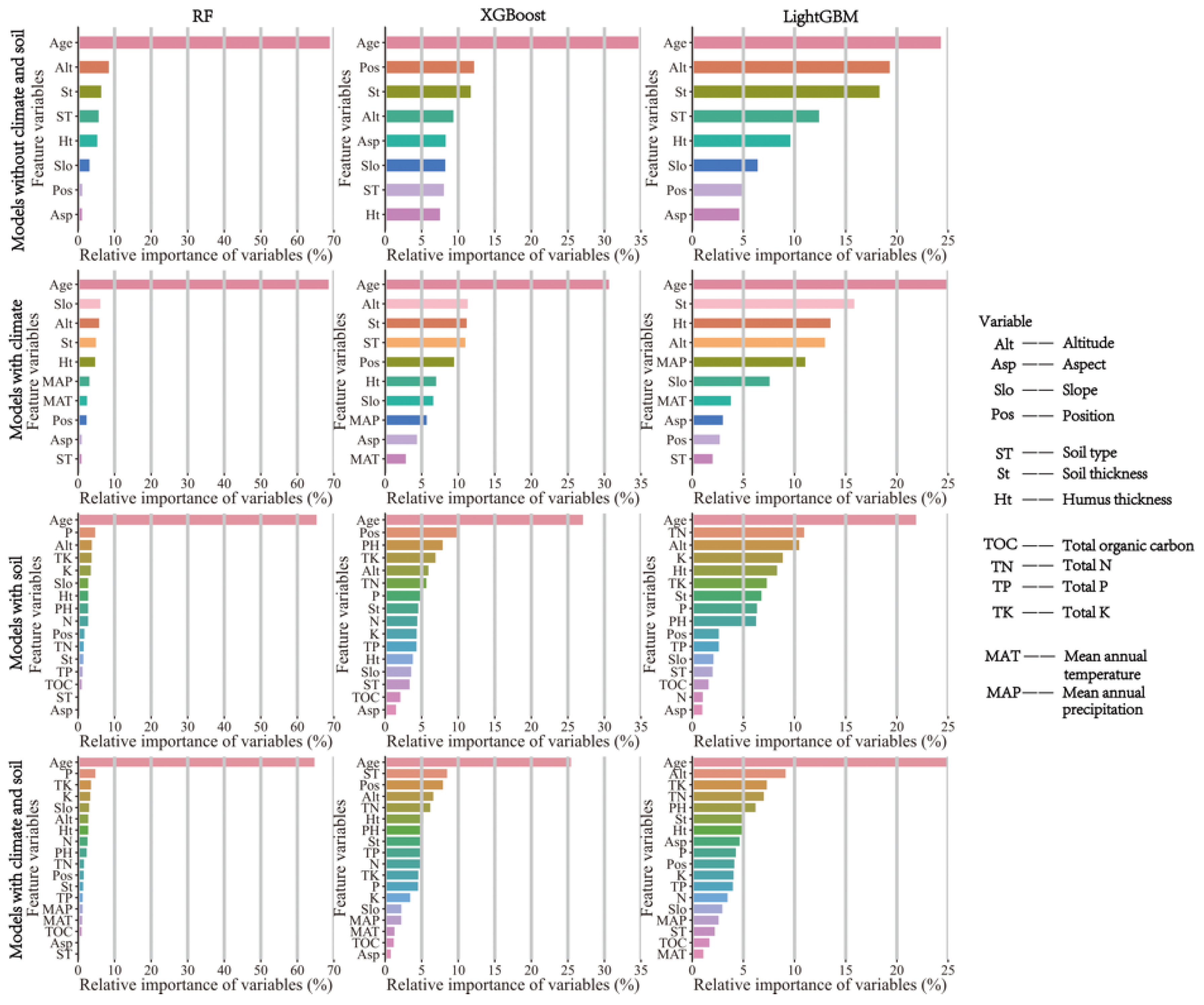
3.2. Variable Importance

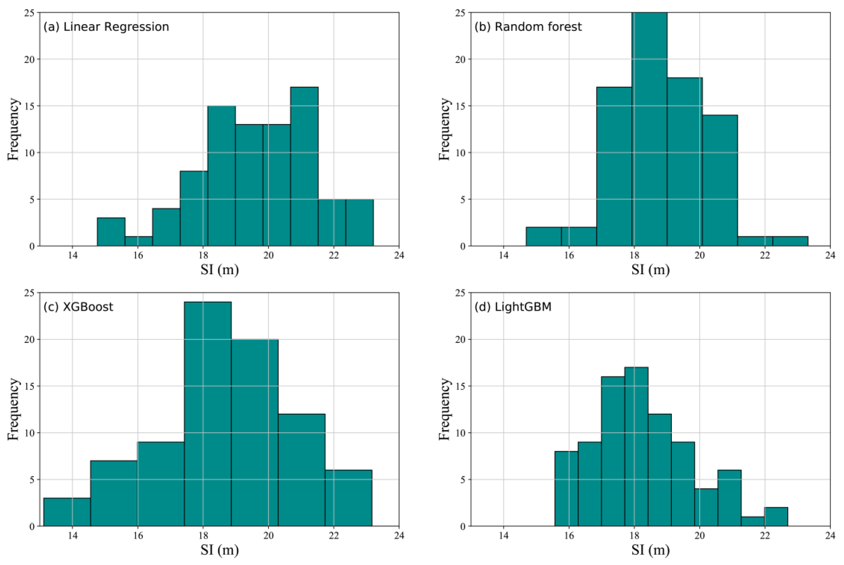
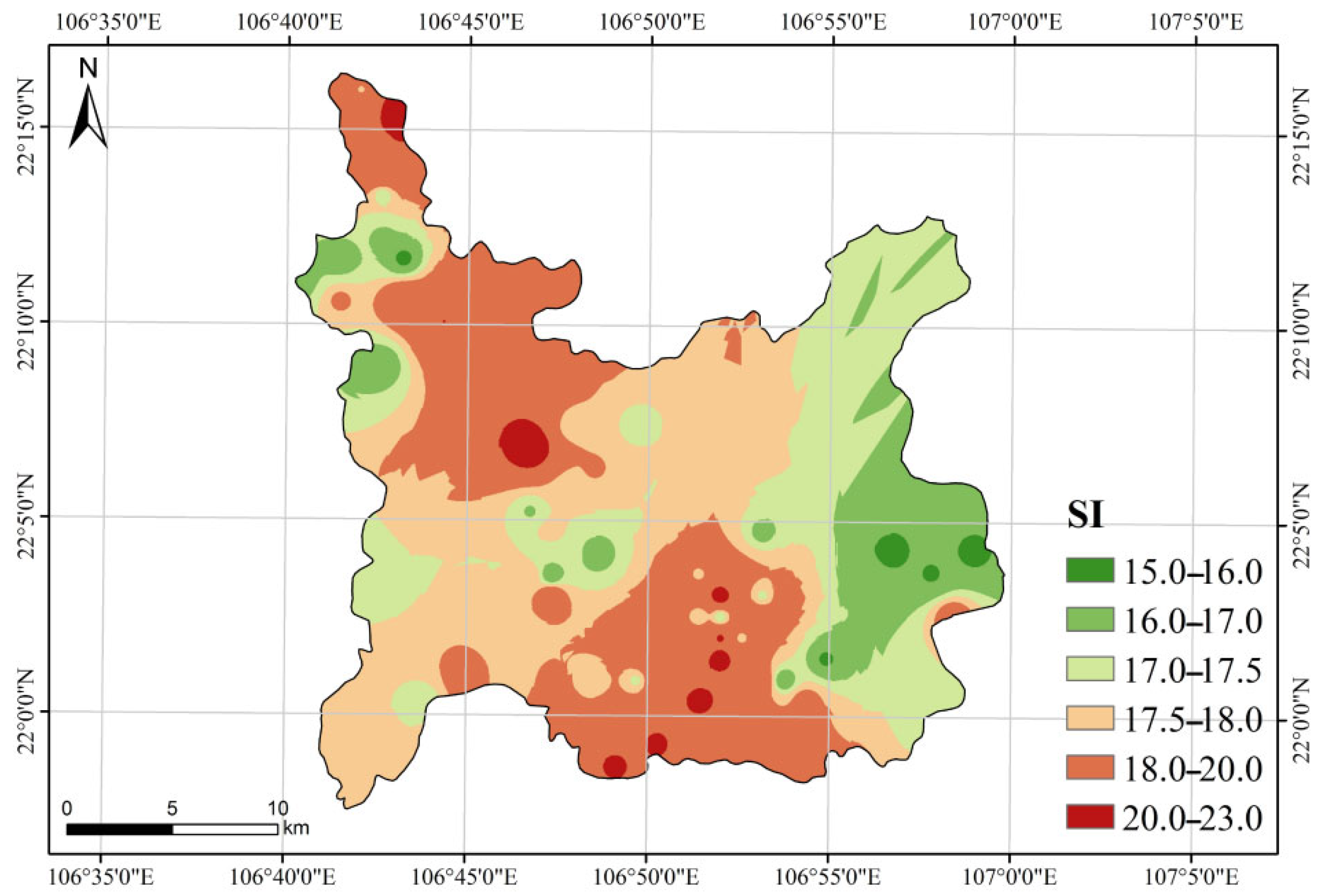
The magnitude of the parameters of each variable reflects the variable importance in a linear model (

Table A3. Parameter values of the variables of the linear regression models.

Variable	Model without Climate and Soil Chemical Variables	Model with Climatic Variables	Model with Soil Chemical Variables	Model with Climatic and Soil Chemical Variables
Age	3.6755	3.6700	3.5780	3.5415
Altitude	−0.6261	−1.0191	0.1406	−1.6870
Aspect	0.1985	0.4049	0.1837	0.2820
Slope	0.3899	0.1693	0.4051	0.1082
Position	0.4629	0.3591	0.3077	0.2520
ST	−0.5486	−0.5974	−0.0729	−0.1289
St	0.3970	0.3234	0.7566	0.8219
Ht	−0.3202	−0.4112	−0.4362	−0.5494
PH	—	—	−1.1538	−1.1094
TOC	—	—	−1.1817	1.1586
TN	—	—	1.6408	1.8775
TP	—	—	0.0050	0.0737
TK	—	—	−0.8459	−0.9823
N	—	—	−1.3421	1.4449
P	—	—	0.5487	0.4990
K	—	—	−0.4861	−0.4168
MAT	—	−0.7778	—	−1.4857
MAP	—	1.2172	—	0.5283

). In contrast, in a machine-learning model, the variable importance is calculated and ranked using a feature importance algorithm (Figure 4). The age ranked first in all models. Therefore, tree height growth models use age as the only variable. The relative importance of age exceeded 60% for all RF models. After the addition of other variables, the elemental content of the soil replaced elevation as the most important environmental variable in the RF models, and the relative importance of age decreased by 4.9%. The importance of age was less than 35% in all XGBoost and LightGBM models, and the environmental variables had more importance. In the XGBoost model that included climate and soil chemical variables, the importance of age was 10% lower, and slope position, soil type, and elevation were the most important environmental variables. The addition of the variables did not substantially change the importance of age in the LightGBM model. However, the importance of elevation and physical properties of the soil was higher in the model without soil chemical properties. The relative importance of age in all models was around 25%. The importance of the climatic variables was lower than that of the soil chemical variables. However, the accuracy of the models with climatic variables was higher than that of the models with only the base data (Table 4). This result suggests that incorporating climatic variables improves model performance and incorporating both climatic and soil chemical variables provides the highest accuracy. We found that the physicochemical properties of the soil had a critical influence on the dominant height of the stand, whereas the climatic variables had a negligible effect.

3.3. SI Prediction

The four models with the highest prediction accuracies using climatic and soil chemical variables were selected to predict the SI based on the baseline age. The width of the bars in Figure 5 indicates the group spacing between the data. The greater the number of groups and the smaller the group spacing, the stronger the continuity of the data. Compared with the other three models, the prediction results of the LightGBM show the most uniform and near-normal distribution (Figure 5). The LightGBM model predictions for the SI show a maximum value of 22.7 m, a minimum value of 15.6 m, a mean value of 18.3 m, a median of 18.1 m, a standard deviation of 1.6 m, a difference of 0.2 m between the median and the mean, and a range of 7.1 m. The SI prediction results (Figure 5) show a normal distribution, with the largest number of sample plots with SI values between 17 and 19 and the smallest number between 21 and 23. Based on the predictions of the LightGBM model, we have made a map of the spatial distribution of the study area for SI (Figure 6). The overall spatial distribution of SI shows a trend of high in the south-eastern and north-western regions and low in the eastern and north-eastern regions.

4. Discussion

Our findings suggest that the LightGBM is an effective method for predicting the SI. Climatic and soil chemical variables were added to the model, and the results were compared with the base scenario model to predict the SI in Masson pine plantations. Four methods (linear regression, RF, XGBoost, and LightGBM) were evaluated. Adding climatic and soil chemical variables to the models improved the prediction accuracy by 13%–20% compared to the base scenario. In models with the same variables, non-parametric models achieved significantly higher accuracy for predicting the SI than traditional parametric methods. These regression tree models are particularly effective for datasets containing a large number of environmental predictors with complex interactions and nonlinear relationships [79], as indicated by the high accuracy achieved in this study. This result is consistent with comparative studies that showed non-parametric models of the SI, such as RF [39], ANNs [41], and XGBoost [57,58], consistently outperformed parametric models. Although non-parametric machine learning models are often more accurate than parametric models, they do have some limitations. Since the prediction process is more closely linked to the data in machine-learning models than in parametric models, the results should not be extrapolated beyond the input conditions [39]. Conversely, regression models can be used to predict data beyond the input data if biologically realistic variables are used and the extrapolation is constrained [57]. In addition, the unsatisfactory performance of XGBoost and RF may also be related to the small sample size. It is well-known that RF and XGBoost tend to achieve satisfactory performance for a large sample size. However, studies in other fields have shown that LightGBM provided satisfactory regression predictions with larger sample sizes [80]. The LightGBM has higher prediction accuracy than XGBoost and RF for small sample sizes [81]. Overall, XGBoost and LightGBM performed better, and the latter was the most accurate model.

We found the LightGBM algorithm suitable for modeling various types of indicators in forestry. New machine learning algorithms have shown good potential for assessing ecological indicators [53,54,55,56]; however, few studies used them for SI prediction. In this study, the LightGBM algorithm outperformed XGBoost and RF but did not perform as well as RF in terms of model bias. RF is a parallel ensemble algorithm based on decision trees that is insensitive to noise during model learning [54,82,83]. XGBoost prevents overfitting by generating a new decision tree based on the previous tree and splitting the leaves of the same layer [54,84]. Unlike XGBoost, LightGBM selects the leaves with the greatest splitting gain and is better able to deal with normalized learning targets, preventing overfitting [78,85]. Predictions using decision tree algorithms are not affected by feature multicollinearity. As a result, the LightGBM not only performed well on the validation set but also had the highest operational efficiency. It saves only the discretized values of the features, significantly reducing memory use [56]. The LightGBM operates better than other machine-learning algorithms in computers with low hardware configurations. In practice, most machine-learning tools do not support categorical variables and require conversion to numerical variables, reducing space and time efficiency. The LightGBM allows for adding decision rules for categorical variables, enabling their direct input without the need for additional 0/n expansion [85]. This method works well for data with many categorical features and correlations between features, which is characteristic of forestry data.

This study used the dominant height of the stand to predict SI. Therefore, the model used the baseline age for determining SI. Several studies predicted SI by modeling environmental factors [38,39,41,57]. The direct acquisition of SI requires time-resolved data for the species in the stand; however, the amount of work required to obtain these data is considerably greater than the direct measurement of stand age. The use of parsed wood data also represents the whole in parts and is therefore subject to modeling errors. Chinese forests are predominantly mixed forests with many tree species rather than pure forests [19]. The influence of the proportions of different tree species on the baseline age of the stand and of the surrounding stands is significant, resulting in large differences in the SI. Therefore, the baseline age can be changed in the proposed SI model based on the dominant height. Thus, this approach is highly applicable to evaluating site productivity in Chinese forests.

Our results obtained from different models provide insights into the extent to which different factors affect the SI. Since machine-learning models do not provide positive or negative significance of the variables, the combination of parameters was based on linear regression models. The effect of different categories of factors are summarized as follows:

(1) Age was the most significant factor influencing the SI.

(2) Most predictors related to the soil layer thickness and soil chemistry were significant, and their incorporation into the model improved the model fit, confirming the importance of including soil physicochemical variables in the SI model [62,63,64,65]. The soil chemical variables had a higher significance level than the soil physical variables, consistent with previous studies [65]. The positive significance of soil nitrogen and phosphorus was attributed to the fact that these elements promote the growth of Masson pine needles [86,87] and affect the abundance of beneficial mycorrhizae [88]. Nitrogen deposition improves stand productivity, explaining the relationship between the age of the Masson pine stand and the SI [89]. The pH, another significant soil chemical variable, was negatively correlated with the SI, in line with the slightly acidic soil conditions common in Masson pine stands. Some interesting differences in the soil variables were observed. The addition of soil chemical variables to most models resulted in a significant reduction in the importance of the soil type variable, suggesting that aspects related to the soil type, e.g., the color, pH, and elemental content, rather than the soil type, were the influencing factors.

(3) The positive and negative significance of the climatic variables, including precipitation and temperature, was consistent with other studies of Masson pine in Guangxi, China [90,91]; however, the significance levels were low. The low significance levels of the climatic factors may be related to the number and distribution of the sample plots, which covered less than a quarter of the total area of the Guangxi region. Related studies have also shown that the larger the regional scale, the more significant the impact of climate change on forest ecosystems was [92,93].

(4) Elevation was the most critical geographical factor. We speculate this is related to the elevation gradient of the sample plots, whose elevation ranged from −122 m to 2233 m above sea level (Figure 1). We found a negative correlation between altitude and SI, corresponding to the elevation gradient of Masson pine. As the elevation increases, the temperature decreases, and low temperatures are not conducive to the growth of Masson pine. When precipitation information (mean annual precipitation) was included in the model, the reliability of the altitude for predicting the SI improved [69].

(5) The spatial distribution of the SI in the study area indicates high stand productivity in the southeast and northwest. It would seem that the cause of this phenomenon may be related to climate and altitude. The study area is located in southern China in the subtropical monsoon climate zone. This region is strongly influenced by the southeast monsoon, which brings suitable temperatures and plenty of moisture. Its path coincides with the SI trend from the southeastern region to the northwestern region. The monsoon does not reach the high-altitude areas in the northeastern and eastern part of the study area, resulting in spatial heterogeneity of the SI. Thus, the stand productivity may decrease in the long term in the eastern and northeastern regions.

Previous studies focused on the effects of stand age, topographic conditions, and soil physical properties on the SI [8,14,19,40] but did not consider the synergistic effects of climatic conditions and soil chemistry. We proposed the LightGMB algorithm to improve the SI prediction accuracy. However, this study has some limitations. First, the relatively small study area prevented us from using other climatic factors, such as air humidity [69], air CO₂ content [61], and solar radiation [57], which might improve the prediction accuracy of the model. Second, the correlation between the variables might have affected the explanatory power of the machine learning models. Using a single site productivity indicator may not be adequate. Combining other site productivity indicators and performing feature selection could improve model accuracy and improve the explanatory power of the variables. In a future study, we will combine the SI with new site productivity indicators, such as site form [94] and the 300 index [57], and use more powerful deep learning algorithms for productivity assessment. We will also be conducting future national scale studies to obtain additional grant funding and research samples to further validate the accuracy and applicability of the machine-learning approach.

5. Conclusions

In this study, we developed SI models with different variables using a parametric approach (multiple linear regression) and three non-parametric machine-learning algorithms (RF, XGBoost, and LightGBM) and compared their performance. The XGBoost and LightGBM models, which included climate and soil chemical variables, were the most suitable for predicting the SI using multiple variables. The LightGBM algorithm outperformed the XGBoost algorithm and explained 67.2% of the variation in the SI, indicating its potential for SI assessment. We considered the effects of climatic conditions and soil physicochemical properties on the SI. The soil physicochemical properties were more reliable than the climatic variables for predicting the SI in Masson pine plantations. The SI depended primarily on the physicochemical properties of the soil, i.e., the nitrogen, phosphorus, and potassium contents, the pH, and the soil layer thickness. We hope that the favorable results obtained from advanced machine-learning algorithms will inspire other studies to combine artificial intelligence with forestry modeling. The proposed SI model with climatic and soil physicochemical variables can also be used for managing unevenly aged Masson pine plantations.

References

1. Ge, X.G.; Xiao, W.F.; Zeng, L.X.; Huang, Z.L.; Lei, J.P.; Li, M.H. The Link Between Litterfall, Substrate Quality, Decomposition Rate, and Soil Nutrient Supply in 30-Year-Old Pinus massoniana Forests in the Three Gorges Reservoir Area, China. Soil Sci. 2013, 178, 442–451. [Google Scholar] [CrossRef]
2. Chen, F.; Yu, J.Y.; Shu, L.Y.; Tong, W.Z. Influence of climate warming and resin collection on the growth of Masson pine (Pinus massoniana) in a subtropical forest, southern China. Trees 2016, 30, 1017. [Google Scholar] [CrossRef] [Green Version]
3. Hu, W.; Yang, X.; Mi, B.; Fang, L.; Tao, Z.; Fei, B.; Jiang, Z.; Liu, Z. Investigating chemical properties and combustion characteristics of torrefied masson pine. Wood Fiber Sci. J. Soc. Wood Sci. Technol. 2017, 49, 33–42. [Google Scholar]
4. Shen, C.; Duan, W.; Cen, B.; Tan, J. Comparison of chemical components of essential oils in needles of Pinus massoniana Lamb and Pinus elliottottii Engelm from Guangxi. Se Pu = Chin. J. Chromatogr. 2006, 24, 619–624. [Google Scholar]
5. Tesch, S.D. The evolution of forest yield determination and site classification. For. Ecol. Manag. 1980, 3, 169–182. [Google Scholar] [CrossRef]
6. Burkhart, H.E.; Tomé, M. Modeling Forest Trees and Stands; Springer: Berlin, Germany, 2012. [Google Scholar]
7. Mcleod, S.D.; Running, S.W. Comparing site quality indices and productivity in ponderosa pine stands of western Montana. Can. J. For. Res. 1988, 18, 346–352. [Google Scholar] [CrossRef]
8. Curt, T.; Bouchaud, M.; Agrech, G. Predicting site index of Douglas-Fir plantations from ecological variables in the Massif Central area of France. For. Ecol. Manag. 2001, 149, 61–74. [Google Scholar] [CrossRef]
9. Louw, J.H.; Scholes, M. Forest site classification and evaluation: A South African perspective. For. Ecol. Manag. 2002, 171, 153–168. [Google Scholar] [CrossRef]
10. Fonweban, J.N.; Tchanou, Z.; Defo, M. Site index equations for Pinus kesiya in Cameroon. J. Trop. For. Sci. 1995, 8, 24–32. [Google Scholar]
11. Skovsgaard, J.P.; Vanclay, J.K. Forest site productivity: A review of the evolution of dendrometric concepts for even-aged stands. Forestry 2008, 81, 13–31. [Google Scholar] [CrossRef] [Green Version]
12. Eichhorn, F. Beziehungen zwischen bestandshöhe und bestandsmasse. Allg. Forst-Und Jagdztg. 1904, 80, 45–49. [Google Scholar]
13. Bontemps, J.D.; Bouriaud, O. Predictive approaches to forest site productivity: Recent trends, challenges and future perspectives. Forestry 2014, 87, 109–128. [Google Scholar] [CrossRef]
14. Pienaar, L.V.; Shiver, B.D. The effect of planting density on dominant height in unthinned slash pine plantations. For. Sci. 1984, 30, 1059–1066. [Google Scholar]
15. Lanner, R.M. On the insensitivity of height growth to spacing. For. Ecol. Manag. 1985, 13, 143–148. [Google Scholar] [CrossRef]
16. Maclaren, J.P.; Grace, J.C.; Kimberley, M.O.; Knowles, R.L.; West, G.G. Height growth of Pinus radiata as affected by stocking. New Zealand. New Zealand. J. Forest. Sci. 1995, 25, 73–90. [Google Scholar]
17. Perron, J. Inventaire forestier. In Manuel de Foresterie; Les Presses de l’Université Laval: Ste-Foy, QC, Canada, 1996; pp. 390–473. [Google Scholar]
18. Lockhart, B.R. Site Index Determination Techniques for Southern Bottomland Hardwoods. South. J. Appl. For. 2013, 37, 5–12. [Google Scholar] [CrossRef]
19. Shen, J.; Wang, Y.; Lei, X.; Lei, Y.; Wang, Q. Site quality evaluation of uneven-aged mixed coniferous and broadleaved stands in Guangdong Province of southern China based on BP neural network. J. Beijing For. Univ. 2019, 4, 38–47, (In Chinese with English abstract). [Google Scholar]
20. Wang, Y.; Lemay, V.M.; Baker, T.G. Modelling and prediction of dominant height and site index of Eucalyptus globulus plantations using a nonlinear mixed-effects model approach. Can. J. For. Res. 2007, 37, 1390–1403. [Google Scholar] [CrossRef]
21. Martin-Benito, D.; Gea-Izquierdo, G.; del Rio, M.; Canellas, I. Long-term trends in dominant-height growth of black pine using dynamic models. For. Ecol. Manag. 2008, 256, 1230–1238. [Google Scholar] [CrossRef]
22. Guo, Y.; Han, Y.; Wu, B.; Yang, L. Study on Modelling of Site Quality Evaluation and its Dynamic Update Technology for Plantation Forests. Nat. Environ. Pollut. Technol. 2013, 12, 591–597. [Google Scholar]
23. Wang, G.G. White spruce site index in relation to soil, understory vegetation, and foliar nutrients. Can. J. For. Res. 1995, 25, 29–38. [Google Scholar] [CrossRef]
24. Chen, H.Y.H.; Krestov, P.V.; Klinka, K. Trembling aspen site index in relation to environmental measures of site quality at two spatial scales. Can. J. For. Res. 2002, 32, 112–119. [Google Scholar] [CrossRef]
25. Sánchez-Rodrıguez, F.; Rodrıguez-Soalleiro, R.; Español, E.; López, C.A.; Merino, A. Influence of edaphic factors and tree nutritive status on the productivity of Pinus radiata D. Don plantations in northwestern Spain. For. Ecol. Manag. 2002, 171, 181–189. [Google Scholar] [CrossRef]
26. Hamel, B.; Bélanger, N.; Paré, D. Productivity of black spruce and Jack pine stands in Quebec as related to climate, site biological features and soil properties. For. Ecol. Manag. 2004, 191, 239–251. [Google Scholar] [CrossRef]
27. Nigh, G.D.; Ying, C.C.; Qian, H. Climate and productivity of major conifer species in the interior of British Columbia, Canada. For. Sci. 2004, 50, 659–671. [Google Scholar]
28. Wang, G.G.; Huang, S.; Monserud, R.A.; Klos, R.J. Lodgepole pine site index in relation to synoptic measures of climate, soil moisture and soil nutrients. For. Chron. 2004, 80, 678–686. [Google Scholar] [CrossRef]
29. Seynave, I.; Gégout, J.-C.; Hervé, J.-C.; Dhôte, J.-F.; Drapier, J.; Bruno, É.; Dumé, G. Picea abies site index prediction by environmental factors and understorey vegetation: A two-scale approach based on survey databases. Can. J. For. Res. 2005, 35, 1669–1678. [Google Scholar] [CrossRef]
30. Monserud, R.A.; Huang, S.; Yang, Y. Predicting lodgepole pine site index from climatic parameters in Alberta. For. Chron. 2006, 82, 562–571. [Google Scholar] [CrossRef]
31. Seynave, I.; Gégout, J.C.; Hervé, J.C.; Dhôte, J.F. Is the spatial distribution of European beech (Fagus sylvatica L.) limited by its potential height growth? J. Biogeogr. 2008, 35, 1851–1862. [Google Scholar] [CrossRef]
32. Socha, J. Effect of topography and geology on the site index of Picea abies in the West Carpathian, Poland. Scand. J. For. Res. 2008, 23, 203–213. [Google Scholar] [CrossRef]
33. Pinno, B.D.; Paré, D.; Guindon, L.; Bélanger, N. Predicting productivity of trem- bling aspen in the Boreal Shield ecozone of Quebec using different sources of soil and site information. For. Ecol. Manag. 2009, 257, 782–789. [Google Scholar] [CrossRef]
34. Watt, M.S.; Palmer, D.J.; Dungey, H.; Kimberley, M.O. Predicting the spatial distribution of Cupressus lusitanica productivity in New Zealand. For. Ecol. Manag. 2009, 258, 217–223. [Google Scholar] [CrossRef]
35. Watt, M.S.; Palmer, D.J.; Kimberley, M.O.; Hock, B.; Payn, T.; Lowe, D. Development of models to predict Pinus radiata productivity throughout New Zealand. Can. J. For. Res. 2010, 40, 488–499. [Google Scholar] [CrossRef]
36. Codilan, A.L.; Nakajima, T.; Tatsuhara, S.; Shiraishi, N. Estimating site index from ecological factors for industrial tree plantation species in Mindanao, Philippines. Bull. Univ. Tokyo For. 2015, 133, 19–41. [Google Scholar]
37. González-Rodríguez, M.A.; Diéguez-Aranda, U. Exploring the use of learning techniques for relating the site index of radiata pine stands with climate, soil and physiography. For. Ecol. Manag. 2020, 458, 117–803. [Google Scholar] [CrossRef]
38. Weiskittel, A.R.; Crookston, N.L.; Radtke, P.J. Linking climate, gross primary productivity, and site index across forests of the western United States. Can. J. For. Res. 2011, 41, 1710–1721. [Google Scholar] [CrossRef]
39. Sabatia, C.O.; Burkhart, H.E. Predicting site index of plantation loblolly pine from biophysical variables. For. Ecol. Manag. 2014, 326, 142–156. [Google Scholar] [CrossRef]
40. Aertsen, W.; Kint, V.; Van Orshoven, J.; Özkan, K.; Muys, B. Comparison and ranking of different modelling techniques for prediction of site index in Mediterranean mountain forests. Ecol. Model. 2010, 221, 1119–1130. [Google Scholar] [CrossRef]
41. Aertsen, W.; Kint, V.; Van Orshoven, J.; Muys, B. Evaluation of modelling techniques for forest site productivity prediction in contrasting ecoregions using stochastic multicriteria acceptability analysis (SMAA). Environ. Modell. Softw. 2011, 26, 929–937. [Google Scholar] [CrossRef] [Green Version]
42. Yu, L.; Lei, X.; Wang, Y.; Yang, Y.; Wang, Q. Impact of climate on individual tree radial growth based on generalized additive model. J. Beijing For. Univ. 2014, 36, 22–32, (In Chinese with English abstract). [Google Scholar]
43. Shen, C.; Lei, X.; Liu, H.; Wang, L.; Liang, W. Potential impacts of regional climate change on site productivity of Larix olgensis plantations in northeast China. iForest Biogeosci. For. 2015, 8, 642. [Google Scholar] [CrossRef]
44. Ou, Q.X.; Lei, X.D.; Shen, C.C. Individual Tree Diameter Growth Models of Larch-Spruce-Fir Mixed Forests Based on Machine Learning Algorithms. Forests 2019, 10, 187. [Google Scholar] [CrossRef] [Green Version]
45. De’Ath, G. Boosted trees for ecological modeling and prediction. Ecology 2007, 88, 243–251. [Google Scholar] [CrossRef]
46. Wu, D.; Jennings, C.; Terpenny, J. A Comparative Study on Machine Learning Algorithms for Smart Manufacturing: Tool Wear Prediction Using Random Forests. J. Manuf. Sci. Eng. Trans. Asme 2017, 139, 7. [Google Scholar] [CrossRef] [Green Version]
47. Wang, H.; Li, Y. Analyzing Variation of Soil Salinity Content in the Agricultural Areas: A Factorial Analysis Based Random Forest Estimation Method. IOP Conf. Ser. Earth Environ. Sci. 2021, 793, 012032. [Google Scholar] [CrossRef]
48. Qiu, Y.G.; Zhou, J.; Khandelwal, M.; Yang, H.T.; Yang, P.X.; Li, C.Q. Performance evaluation of hybrid WOA-XGBoost, GWO-XGBoost and BO-XGBoost models to predict blast-induced ground vibration. Eng. Comput. 2021, 1–18. [Google Scholar] [CrossRef]
49. Sun, B.; Sun, T.; Jiao, P.P. Spatio-Temporal Segmented Traffic Flow Prediction with ANPRS Data Based on Improved XGBoost. J. Adv. Transp. 2021, 1, 1–24. [Google Scholar] [CrossRef]
50. Zhan, Z.H.; You, Z.H.; Li, L.P.; Zhou, Y.; Yi, H.C. Accurate Prediction of ncRNA-Protein Interactions From the Integration of Sequence and Evolutionary Information. Front. Genet. 2018, 9, 458. [Google Scholar] [CrossRef]
51. Deng, X.S.; Li, M.; Deng, S.B.; Wang, L. Hybrid gene selection approach using XGBoost and multi-objective genetic algorithm for cancer classification. Med. Biol. Eng. Comput. 2021, 60, 663–681. [Google Scholar] [CrossRef]
52. Ahirwal, J.; Nath, A.; Brahma, B.; Deb, S.; Sahoo, U.K.; Nath, A.J. Patterns and driving factors of biomass carbon and soil organic carbon stock in the Indian Himalayan region. Sci. Total Environ. 2021, 770, 145292. [Google Scholar] [CrossRef]
53. Wang, Z.G.; Wang, G.C.; Zhang, G.H.; Wang, H.B.; Ren, T.Y. Effects of land use types and environmental factors on spatial distribution of soil total nitrogen in a coalfield on the Loess Plateau, China. Soil Tillage Res. 2021, 211, 105027. [Google Scholar] [CrossRef]
54. Luo, M.; Wang, Y.F.; Xie, Y.H.; Zhou, L.; Qiao, J.J.; Qiu, S.Y.; Sun, Y.J. Combination of Feature Selection and CatBoost for Prediction: The First Application to the Estimation of Aboveground Biomass. Forests 2021, 12, 216. [Google Scholar] [CrossRef]
55. Effrosynidis, D.; Tsikliras, A.; Arampatzis, A.; Sylaios, G. Species Distribution Modelling via Feature Engineering and Machine Learning for Pelagic Fishes in the Mediterranean Sea. Appl. Sci. 2020, 10, 8900. [Google Scholar] [CrossRef]
56. Effrosynidis, D.; Arampatzis, A. An evaluation of feature selection methods for environmental data. Ecol. Inform. 2021, 61, 101224. [Google Scholar] [CrossRef]
57. Watt, M.S.; Palmer, D.J.; Leonardo, E.; Bombrun, M. Use of advanced modelling methods to estimate radiata pine productivity indices. For. Ecol. Manag. 2021, 479, 118–557. [Google Scholar] [CrossRef]
58. Gavilán-Acuña, G.; Olmedo, G.F.; Mena-Quijada, P.; Guevara, M.; Barría-Knopf, B.; Watt, M.S. Reducing the Uncertainty of Radiata Pine Site Index Maps Using an Spatial Ensemble of Machine Learning Model. Forests 2021, 12, 77. [Google Scholar] [CrossRef]
59. Watt, M.S.; Dash, J.P.; Bhandari, S.; Watt, P. Comparing parametric and non-parametric methods of predicting Site Index for radiata pine using combinations of data derived from environmental surfaces, satellite imagery and airborne laser scanning. For. Ecol. Manag. 2015, 357, 1–9. [Google Scholar] [CrossRef]
60. Bravo-Oviedo, A.; Roig, S.; Bravo, F.; Montero, G.; Del-Rio, M. Environmental variability and its relationship to site index in Mediterranean maritine pine. For. Syst. 2011, 20, 50–64. [Google Scholar] [CrossRef]
61. Sharma, R.P.; Brunner, A.; Eid, T. Site index prediction from site and climate variables for Norway spruce and Scots pine in Norway. Scand. J. For. Res. 2012, 27, 619–636. [Google Scholar] [CrossRef]
62. Carmean, W.H. Forest site quality evaluation in the United States. Adv. Agron. 1975, 27, 209–269. [Google Scholar]
63. Turner, J.; Thompson, C.H.; Turvey, N.D.; Hopmans, P.; Ryan, P.J. A soil technical classification for Pinus radiata (D. Don) plantations. I. Development. Aust. J. Soil Res. 1990, 28, 797–811. [Google Scholar] [CrossRef]
64. Ritchie, M.W.; Hamann, J.D. Individual-tree height-, diameter- and crown-width increment equations for young Douglas-fir plantations. New For. 2008, 35, 173–186. [Google Scholar] [CrossRef]
65. Grigal, D.F. A soil-based aspen productivity index for Minnesota. For. Ecol. Manag. 2009, 257, 1465–1473. [Google Scholar] [CrossRef]
66. Wang, T.L.; Hamann, A.; Spittlehouse, D.L.; Murdock, T.Q. ClimateWNA—High-Resolution Spatial Climate Data for Western North America. J. Appl. Meteorol. Climatol. 2012, 51, 16–29. [Google Scholar] [CrossRef] [Green Version]
67. Hamann, A.; Wang, T.L.; Spittlehouse, D.L.; Murdock, T.Q. A comprehensive, high-resolution database of historical and projected climate surfaces for western north america. Bull. Am. Meteorol. Soc. 2013, 94, 1307–1309. [Google Scholar] [CrossRef]
68. Wang, T.L.; Innes, G.Y.; Seely, J.L.; Chen, B.Z. ClimateAP: An application for dynamic local downscaling of historical and future climate data in Asia Pacific. Front. Agr. Sci. Eng. 2017, 4, 448–458. [Google Scholar] [CrossRef] [Green Version]
69. Grant, J.C.; Nichols, J.D.; Smith, R.G.B.; Brennan, P.; Vanclay, J.K. Site index prediction of Eucalyptus dunnii Maiden plantations with soil and site parameters in sub-tropical eastern Australia. Aust. For. 2010, 73, 234–245. [Google Scholar] [CrossRef]
70. Merian, P.; Lebourgeois, F. Size-mediated climate-growth relationships in temperate forests: A multi-species analysis. For. Ecol. Manag. 2013, 261, 1382–1391. [Google Scholar] [CrossRef]
71. Lei, X.D.; Yu, L.; Hong, L.X. Climate-sensitive integrated stand growth model (CS-ISGM) of Changbai larch (Larix olgensis) plantations. For. Ecol. Manag. 2016, 376, 265–275. [Google Scholar] [CrossRef]
72. Xiang, W.; Lei, X.D.; Zhang, X.Q. Modelling tree recruitment in relation to climate and competition in semi-natural Larix-Picea-Abies forests in northeast China. For. Ecol. Manag. 2016, 382, 100–109. [Google Scholar] [CrossRef]
73. Danescu, A.; Albrecht, A.T.; Bauhus, J.; Kohnle, U. Geocentric alternatives to site index for modeling tree increment in uneven-aged mixed stands. For. Ecol. Manag. 2017, 392, 1–12. [Google Scholar] [CrossRef]
74. Breiman, L. Random Forests. Mach. Learn. 2001, 45, 5–32. [Google Scholar] [CrossRef]
75. Chen, T.; Guestrin, C. XGBoost: A Scalable Tree Boosting System. In Proceedings of the 22nd ACM SIGKDD International Conference on Knowledge Discovery and Data Mining, San Francisco, CA, USA, 13–17 August 2016; Association for Computing Machinery: New York, NY, USA, 2016; Volume 785, p. 794. [Google Scholar]
76. Jin, Q.; Fan, X.; Liu, J.; Xue, Z.; Jian, H. Estimating Tropical Cyclone Intensity in the South China Sea Using the XGBoost Model and FengYun Satellite Images. Atmosphere 2020, 11, 423. [Google Scholar] [CrossRef] [Green Version]
77. Samat, A.; Li, E.; Wang, W.; Liu, S.; Lin, C.; Abuduwaili, J. Meta-XGBoost for Hyperspectral Image Classification Using Extended MSER-Guided Morphological Profiles. Remote Sens. 2020, 12, 1973. [Google Scholar] [CrossRef]
78. Ke, G.; Meng, Q.; Finley, T.; Wang, T.; Chen, W.; Ma, W.; Ye, Q.; Liu, T.-Y. Lightgbm: A highly efficient gradient boosting decision tree. Adv. Neural Inf. Proces. Syst. 2017, 39, 3146–3154. [Google Scholar]
79. Strobl, C.; Malley, J.; Tutz, G. An introduction to recursive partitioning: Rationale, application, and characteristics of classification and regression trees, bagging, and random forests. Psychol. Meth. 2009, 14, 323. [Google Scholar] [CrossRef] [Green Version]
80. Shehadeh, A.; Alshboul, O.; Al Mamlook, E.; Hamedat, O. Machine learning models for predicting the residual value of heavy construction equipment: An evaluation of modified decision tree, LightGBM, and XGBoost regression. Autom. Constr. 2021, 129, 103827. [Google Scholar] [CrossRef]
81. Yan, F.; Song, K.; Liu, Y.; Chen, S.; Chen, J. Predictions and mechanism analyses of the fatigue strength of steel based on machine learning. J. Mater. Sci. 2020, 55, 15334–15349. [Google Scholar] [CrossRef]
82. Li, M.; Zhang, Y.; Wallace, J.; Campbell, E. Estimating annual runoff in response to forest change: A statistical method based on random forest. J. Hydrol. 2020, 589, 125168. [Google Scholar] [CrossRef]
83. Montorio, R.; Perez-Cabello, F.; Alves, D.B.; Garcia-Martin, A. Unitemporal approach to fire severity mapping using multispectral synthetic databases and Random Forests. Remote Sens. Environ. 2020, 249, 112025. [Google Scholar] [CrossRef]
84. Dong, H.; Xu, X.; Wang, L.; Pu, F. Gaofen-3 PolSAR Image Classification via XGBoost and Polarimetric Spatial Information. Sensors 2018, 18, 611. [Google Scholar] [CrossRef] [Green Version]
85. Bentejac, C.; Csorgo, A.; Martinez-Munoz, G. A comparative analysis of gradient boosting algorithms. Artif. Intell. Rev. 2021, 54, 1937–1967. [Google Scholar] [CrossRef]
86. Koerselman, W.; Meuleman, A.F.M. The vegetation N:P ratio: A new tool to detect the nature of nutrient limitation. J. Appl. Ecol. 1996, 33, 1441–1450. [Google Scholar] [CrossRef]
87. Wright, I.J.; Reich, P.B.; Westoby, M.; Ackerly, D.; Baruch, Z.; Bongers, F.; Cavender-Bares, J.; Chapin, T.; Cornelissen, J.; Diemer, M. 2004. The worldwide leaf economics spectrum. The worldwide leaf economics spectrum. Nature 2004, 428, 821–827. [Google Scholar]
88. Yu, H.; Chen, Z.; Shang, H.; Cao, J. Effects of ectomycorrhizal fungi on seedlings of Pinus massoniana under simulated acid rain. Acta Ecol. Sin. 2017, 37, 5418–5427, (In Chinese with English abstract). [Google Scholar]
89. Tyminska-Czabanska, L.; Socha, J.; Maj, M.; Cywicka, D.; Duong, X.V.H. Environmental Drivers and Age Trends in Site Productivity for Oak in Southern Poland. Forests 2021, 12, 209. [Google Scholar] [CrossRef]
90. Zhang, L.; Liu, X.; Su, Y.; Xia, W.; Liang, J. Research progress on the biomass and productivity of Pinus Massoniana plantation. Ecol. Sci. 2018, 37, 213–221, (In Chinese with English abstract). [Google Scholar]
91. Qin, J.; Li, Y.; Ma, J.; Lan, C.; Li, H. Biomass model construction and distribution pattern of Pinus Massoniana plantations under different climatic conditions in Guangxi. Guangxi Sci. 2020, 27, 165–174, (In Chinese with English abstract). [Google Scholar]
92. Mahlstein, I.; Knutti, R. Regional climate change patterns identified by cluster analysis. Clim. Dyn. 2010, 35, 587–600. [Google Scholar] [CrossRef] [Green Version]
93. Dunckel, K.; Weiskittel, A.; Fiske, G. Projected Future Distribution of Tsuga canadensis across Alternative Climate Scenarios in Maine, U.S. Forests 2017, 8, 285. [Google Scholar] [CrossRef]
94. Ahmadi, K.; Alavi, S.J.; Kouchaksaraei, M.T. Constructing site quality curves and productivity assessment for uneven-aged and mixed stands of oriental beech (Fagus oriental Lipsky) in Hyrcanian forest, Iran. For. Sci. Technol. 2017, 13, 41–46. [Google Scholar]
Figure 1. Distribution of sampling plots at the Tropical Forestry Experimental Centre.
Forests 13 01976 g001
Figure 2. Sample plot design of the Tropical Forestry Experimental Centre.
Forests 13 01976 g002
Figure 3. Scatterplot of the predicted and observed dominant height of the stand (SDH) obtained from linear regression, RF, XGBoost, and LightGBM for models with different variables. The dotted blue line is the 1:1 line, and the solid red line is the fitted line (only the best prediction interval line segment is retained). (a,c,e,g) are the basic models; (b,d,f,h) are the models with the climate and soil chemical variables; (i,k,m,o) are the models with the climate variables; (j,l,n,p) are the models with the soil variables.
Forests 13 01976 g003
Figure 4. Ranking of the importance of different types of variables affecting the dominant height of the stand of Pinus massoniana using machine-learning algorithms (RF, XGBoost, and LightGBM).
Forests 13 01976 g004
Figure 5. Frequency histogram of predicted SI for the four models using climatic and soil chemical variables.
Forests 13 01976 g005
Figure 6. Map of the SI.
Forests 13 01976 g006