Article

A Comparative Study of Shallow Machine Learning Models and Deep Learning Models for Landslide Susceptibility Assessment Based on Imbalanced Data

1
School of Information Engineering, Huzhou University, Huzhou 313000, China
2
School of Information Engineering, East China University of Technology, Nanchang 330013, China
*
Author to whom correspondence should be addressed.
Forests 2022, 13(11), 1908; https://doi.org/10.3390/f13111908
Submission received: 12 October 2022 / Revised: 9 November 2022 / Accepted: 11 November 2022 / Published: 14 November 2022
(This article belongs to the Special Issue Landslides in Forests around the World: Causes and Mitigation)

Abstract

:
A landslide is a type of geological disaster that poses a threat to human lives and property. Landslide susceptibility assessment (LSA) is a crucial tool for landslide prevention. This paper’s primary objective is to compare the performances of conventional shallow machine learning methods and deep learning methods in LSA based on imbalanced data to evaluate the applicability of the two types of LSA models when class-weighted strategies are applied. In this article, logistic regression (LR), random forest (RF), deep fully connected neural network (DFCNN), and long short-term memory (LSTM) neural networks were employed for modeling in the Zigui-Badong area of the Three Gorges Reservoir area, China. Eighteen landslide influence factors were introduced to compare the performance of four models under a class balanced strategy versus a class imbalanced strategy. The Spearman rank correlation coefficient (SRCC) was applied for factor correlation analysis. The results reveal that the elevation and distance to rivers play a dominant role in LSA tasks. It was observed that DFCNN (AUC = 0.87, F1-score = 0.60) and LSTM (AUC = 0.89, F1-score = 0.61) significantly outperformed LR (AUC = 0.89, F1-score = 0.50) and RF (AUC = 0.88, F1-score = 0.50) under the class imbalanced strategy. The RF model achieved comparable outcomes (AUC = 0.90, F1-score = 0.61) to deep learning models under the class balanced strategy and ran at a faster training speed (up to 63 times faster than deep learning models). The LR model performance was inferior to that of the other three models under the balanced strategy. Meanwhile, the deep learning models and the shallow machine learning models showed significant differences in susceptibility spatial patterns. This paper’s findings will aid researchers in selecting appropriate LSA models. It is also valuable for land management policy making and disaster prevention and mitigation.

1. Introduction

A landslide is one of the most destructive geological disasters around the world. Landslides are widely distributed in mountainous and reservoir bank areas, which seriously threaten people’s lives and property safety. Landslide susceptibility assessment (LSA) evaluates potential landslides spatially, which is an important tool for landslide prevention. LSA selects a series of landslide influence factors and estimates the probability of landslide occurrence. The LSA models typically work with the geographic information system (GIS) frameworks [1,2] and are grouped into two categories: model-driven and data-driven models. Model-driven LSA models can be expressed by mathematical formulas and are driven by physical theories; for instance, the shallow landslide stability model (SHALTAB) model assumes that the intensity of rainfalls remains constant and the rain seeps into the ground completely [3,4]. For model-driven LSA models, specific geotechnical parameters are necessary [5,6,7].
According to the literature review, data-driven models are the most common methods for LSA. The data-driven models are classified into two groups: knowledge-based models and machine learning models. For knowledge-based models [8], domain expertise is requested from the experts; they need to assign weights to landslide influence factors based on their expertise or available literature [9].
Machine learning techniques play a crucial role in data-driven models, and they are the most widely used approaches for LSA [10]. In general, machine learning approaches consist of two phases: training and testing. During the training phase, the input features and the targets are sent into the models, and the inner parameters of the models are fine-tuned according to some specified rules. The targets are predicted based on the trained models during the testing phase. The representative machine learning approaches involve frequency ratio [11], logistic regression (LR) [12,13], support vector machine (SVM) [14], Bayesian network (BN) [15], random forest (RF) [16,17], back propagation network (BP) [18,19], and ensemble learning techniques [20,21]. These models are the so-called shallow machine learning methods, which have the ability to handle more complex data than knowledge-based approaches [22]. These models can be integrated with other models to provide better performance [23]. Furthermore, it is observed that combining data-driven machine learning methods with qualitative analysis can improve the reliability of LSA models [24].
In recent years, deep learning approaches have demonstrated surprising feature extraction and data fitting capabilities and they are applied in the fields of computer vision [25], natural language processing [26], autopiloting [27], and intelligent medicine [28]. Recent literature describes deep learning approaches as a potent tool for LSA, attracting the interest of numerous researchers [29,30,31,32]. Prior research has demonstrated that LSA models based on deep learning techniques outperform LSA models based on shallow machine learning techniques [33,34]. The convolutional neural network (CNN) is the most widely used deep learning algorithm [33]. The authors of [35] applied CNN to Jiuzhaigou, Sichuan province, China, and verified that CNN achieved better performance compared with multi-layer perceptron (MLP). The authors of [36] developed a 1D-CNN with a high dropout rate to evaluate landslide susceptibility in South Korea. The results showed that 1D-CNN outperformed the artificial neural networks (ANN) and SVM because of its sophisticated architecture. Other deep learning approaches, including deep belief networks (DBN) and recurrent neural networks (RNNs), were also applied for LSA and achieved promising performances [30,32].
In the real world, the number of non-landslide samples is far more than the number of landslide samples. Many researchers have examined various LSA models, and most of them have utilized a balanced sampling technique in the training stage, which involves selecting an equal number of data from both landslide and non-landslide occurrences at random [37]. Without a doubt, this sampling technique is quite useful and effective [38,39]. However, the sampling technique introduces additional complexity to LSA models. A class-weighted strategy is a simple and effective solution to address the problem of imbalanced data in LSA [40]. The class-weighted strategies are mainly discussed in conventional machine learning LSA models and rarely reported in deep learning LSA models. Are the class-weighted strategies still effective for the deep learning LSA models? Additionally, in the scenario of extremely imbalanced data, do the deep learning LSA models outperform conventional shallow machine learning LSA models? To bridge this gap, the real-world matched imbalanced data were used as the training dataset to compare the landslide and the non-landslide evaluation performances based on shallow LSA models and deep LSA models. The Three Gorges reservoir area was chosen as the study area in this paper, which then employed the SRCC approach to assess the correlation between various landslide influence factors, and finally selected the informative factors to build LSA models. Two conventional shallow machine learning models, LR and RF, and two typical deep learning models, DFCNN and LSTM, were employed as LSA models. The performances of these models were assessed using the area under curve (AUC) and the F1-score for various landslide to non-landslide class-weight ratios. Finally, this research concludes with some insightful recommendations for the selection of LSA models based on the experimental findings.

2. Materials

2.1. Study Area

The study area is located in the Zigui-Badong section of the Three Gorges Reservoir area, Hubei Province, China, with a longitude between 110°15′51″ E and 110°52′33″ E and a latitude between 30°51′21″ N and 31°5′1″ N (Figure 1). There are a large number of mountains, valleys, and hills in the study area, with a total area of 662.671 km2 and a maximum altitude of 2004 m. The main stream of the Yangtze River flows through the whole area. Landslides are mainly distributed on both sides of the main stream and tributaries of the Yangtze River. According to the field survey data, there have been 332 identified slides (stable and unstable), with a total area of about 4210 m2. These historical landslides include soil landslides, rock landslides, rock and soil mixed landslides, and other types of landslides, which accounted for 53%, 37%, 2%, and 8% of the total area, respectively.
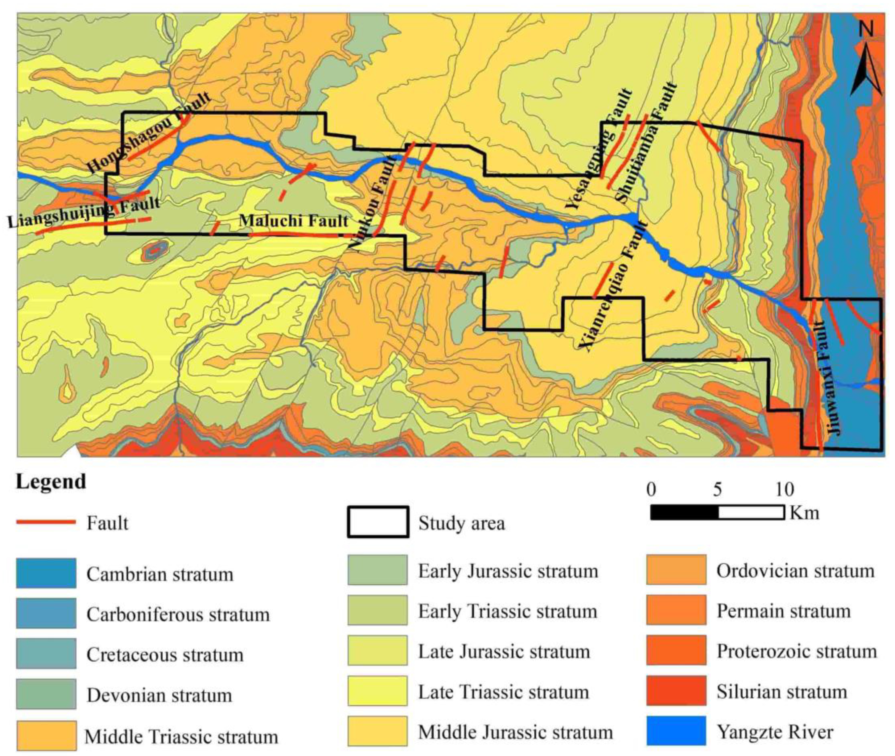
The study area is mainly located in the pre-Nanhua metamorphic basement area at the core of the Huangling dome and the surrounding sedimentary cover area in the south, which belongs to the Yangtze Craton core area in South China. The strata in the study area are well developed and gradually new from east to west. The strata are mainly composed of the Badong Formation. The principal composition of the Badong Formation is an argillaceous rock with low mechanical strength and weak weathering resistance, which makes the formation prone to geological disasters. The Badong Formation in the study area belongs to the middle Triassic (Figure 2). The overlying strata are the Xujiahe Formation, Jiuligang Formation, and Shazhenxi Formation of the Upper Triassic, and the underlying strata are the Jialingjiang Formation of the Lower Triassic.
The study area has abundant rainfall, and the monthly average rainfall can exceed 1000 mm. Heavy rainfall leads to a considerable increase of water content in soil, which is a key influence factor inducing landslides. Meanwhile, the Xiannvshan fault, the Niukou fault, and other small faults are also located in the study area. The rock stratum along the fault zone is squeezed and stretched, and the stratum instability increases, which controls the generation of landslides around the fault zone.

2.2. Data Source

In this research, Landsat 8 OLI remote sensing images (2013) were used to extract the land cover factor, and a 1:50,000 geological map was utilized to derive the geological and hydrological related factors. Elevation data were derived from an ASTER GDEM V2 image, and rainfall data were collected from Climate Hazards Group InfraRed Precipitation with Station data (CHIRPS) (2013). Seismic data were collected from 1978 to 2013. In addition, landslide inventory data from field surveys were available. On the basis of the original data, all influence factors were vectorized, rasterized, and converted into raster layers prior to model computation. All the influence raster layers were resampled to 30 × 30 m using the nearest neighbor sampling technique to match the resolution of elevation data and Landsat images.

3. Methodology

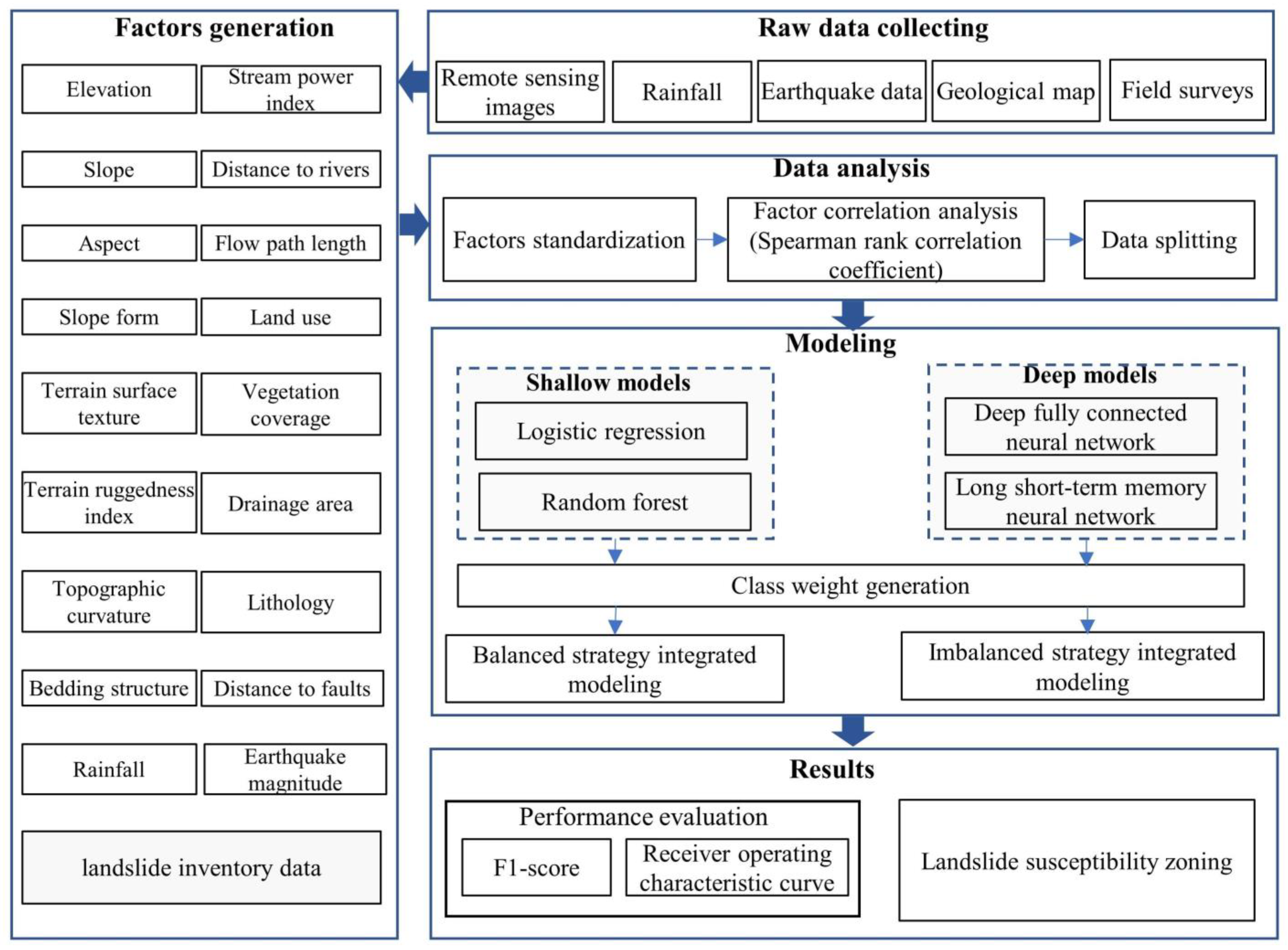
In the present study, the LSA modeling involves four principal steps (Figure 3): (1) collecting the raw data, (2) data preparation, which includes landslide influence factors generation, factors standardization, factor correlation analysis and data splitting, (3) modeling based on two shallow machine learning models and two deep learning models, (4) performance evaluation and landslide susceptibility zoning of the study areas.

3.1. Landslide Susceptibility Models

3.1.1. Logistic Regression

Logistic regression (LR) has been widely used in landslide susceptibility assessment [41,42,43]. In general, y = w 1 x 1 + w 2 x 2 + + w n x n + b is used for the linear fitting of data. Landslide susceptibility assessment is a nonlinear binary classification problem. Thus, a nonlinear mapping is required to be applied to y. The sigmoid function is generally used to add nonlinear characteristics to y. The sigmoid function is defined as Equation (1) [44].
g ( y ) = 1 1 + e y = 1 1 + e ( w 1 x 1 + w 2 x 2 + + w n x n )
The above equation will make the model’s output range from 0 to 1. An output value close to 0 means samples are classified as non-landslide. An output value close to 1 means samples are classified as landslides. To facilitate calculation, the logarithm of the above equation is usually taken.

3.1.2. Random Forest

Random forest (RF) [45,46,47] is an ensemble learning model that integrates multiple weak decision tree models to form a robust classification model. RF picks the input samples and features randomly, so it can avoid over-fitting problems to a certain extent and has good anti-noise abilities. The RF construction processes are summarized as following steps:
(1)
Random sample selection. Assume that the total number of samples is N and there are m decision trees in RF; to create subset N s , select s samples from N samples randomly; a total of m sample subsets are constructed.
(2)
Random feature selection. Assume that the total number of features is F , and h features are selected from the F to form a feature subset F h . The optimal feature is generated from the feature subset F h when the decision tree splits each time.
(3)
Classifier voting. m decision trees produce a total number of m classification results. The class with the highest votes is used as the final prediction class.

3.1.3. Deep Fully Connected Neural Network

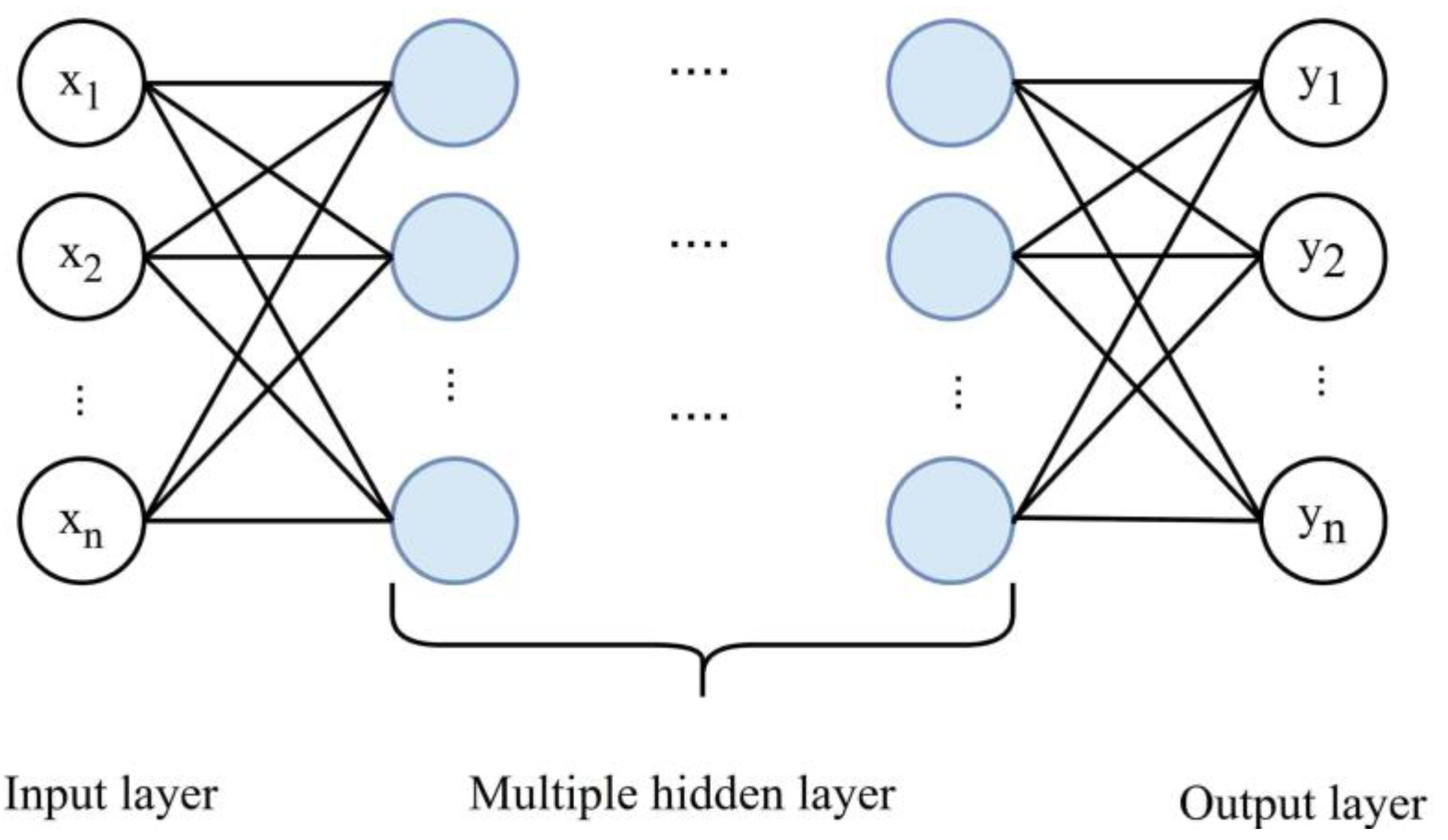
Conventional shallow neural networks generally consist of three layers, which are the input layer, the hidden layer, and the output layer [48]. There are connections between the nodes of the previous layer and those of the following layer. The data fitting ability of a three-layer neural network is limited due to its shallow structure in practice. The deep fully connected neural network (DFCNN) builds a deeper structure by adding extra hidden layers to the basic three-layer structure. The structure of the DFCNN is shown in Figure 4.
The input of the network is [ x 1 , x 2 , , x n ] , and the weights w and the bias b are generally applied to the inputs. To make the neurons have nonlinear mapping capabilities, it is common to send the outputs of the neurons to an activation function, σ . The process can be expressed by the following Equation (2) [49].
h = δ ( i = 1 n w i x i + b )
The commonly used activation functions are the sigmoid function, the tanh function, and the rectified linear units (ReLU) [50] function. Since the sigmoid function and tanh function have the problem of gradient vanishing, the ReLU function was adopted in this article. The derivative of ReLU is 1 while the inputs are greater than 0, which maintains the gradient without decay. The ReLU function alleviates the gradient vanishing problem to a certain extent. The definition of the ReLU function is indicated by Equation (3).
f ( x ) = { x , x 0 0 , x < 0
Since landslide susceptibility assessment is a binary classification problem, the last output layer is connected to a sigmoid function that outputs the probability value for each class.

3.1.4. Long Short-Term Memory Neural Network

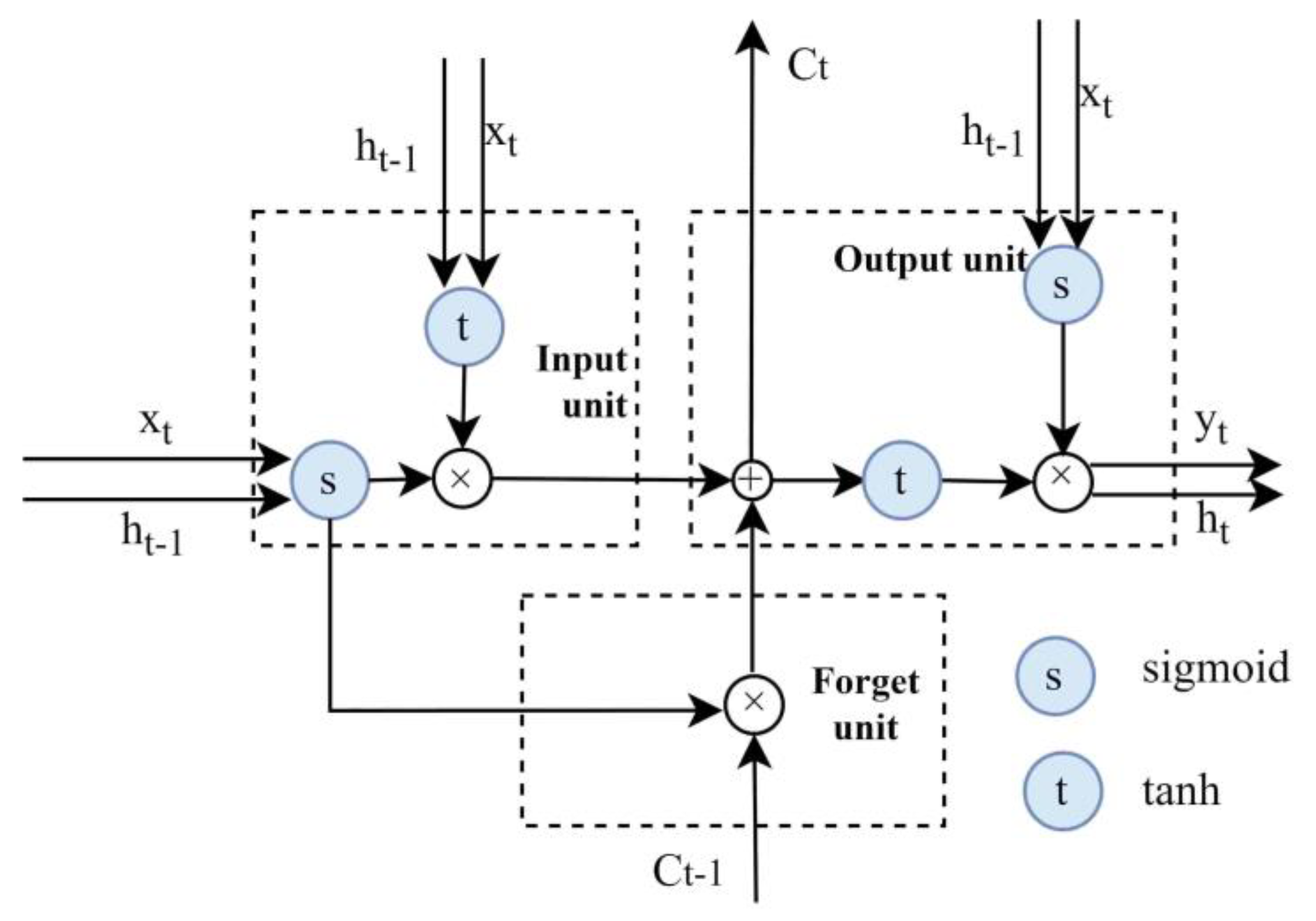
A long short-term memory (LSTM) neural network [51] is a special recurrent neural network (RNN) [52]. An RNN has a loop in the hidden layer, which sends the information from the previous hidden layer into the current hidden layer. It represents that there exists a connection between the nodes at different time points. However, for long sequences, a RNN still has the gradient vanishing problem. To address this problem, LSTM adopts a gating mechanism to control the state of information flow, which is called “memory block”. There are three types of gating units in the memory block: input gate, forget gate, and output gate. The input gate selectively retains the essential information, the forget gate filters the irrelevant or interfering information, and the output gate integrates information together and outputs them. The architecture of the memory block is indicated in Figure 5.
In Figure 5, x t represents the original input at time step t , h t 1 is the hidden layer state transmitted from time step t 1 , and C t 1 is the memory block state transmitted at time step t 1 . After passing through the memory block, three results, y t , h t and C t , are generated, which are the class output at time step t , the hidden layer output at time step t , and the memory block state output at time step t , respectively. Sigmoid and tanh activation functions are used in memory blocks to obtain nonlinear mapping abilities.

3.2. Landslide Influence Factors

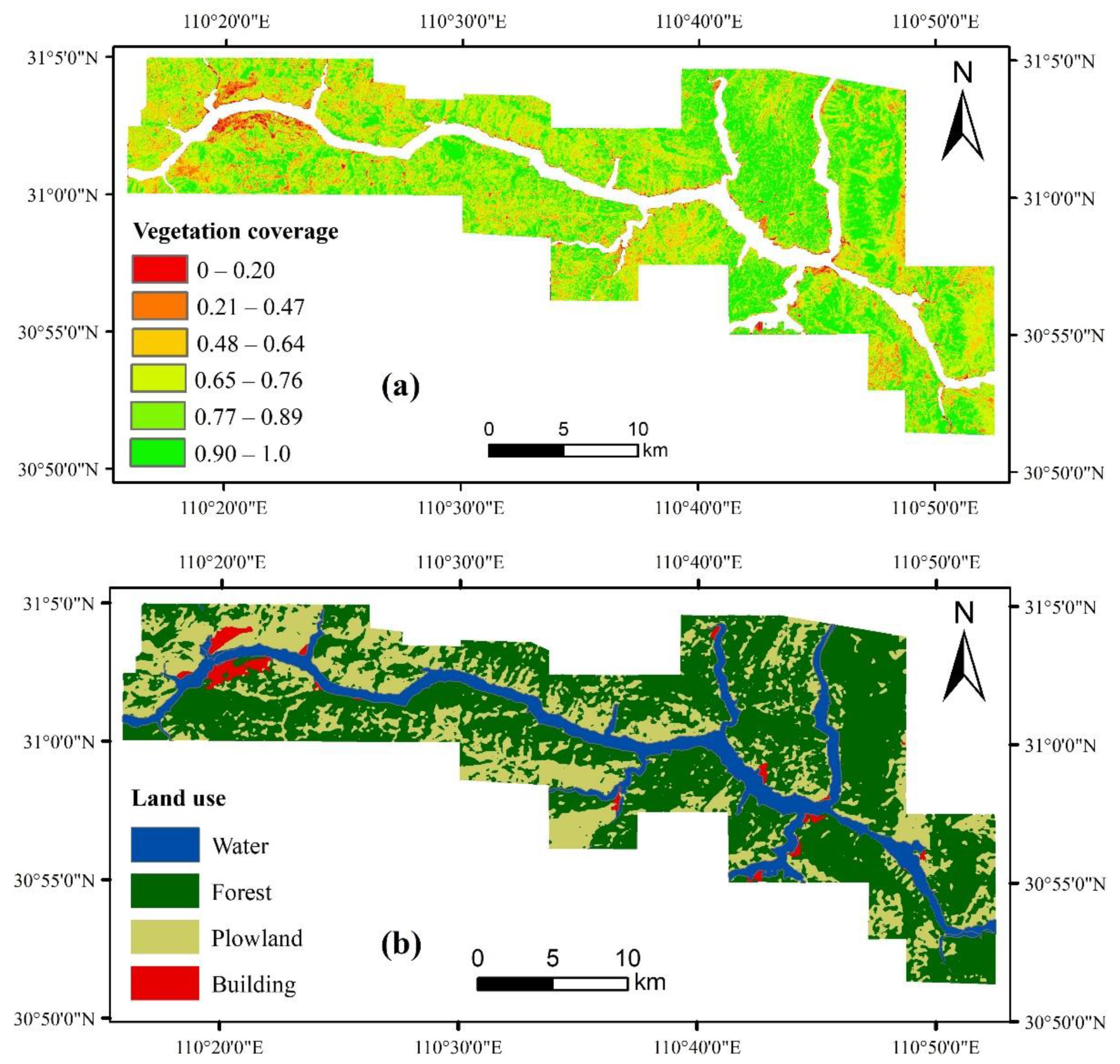
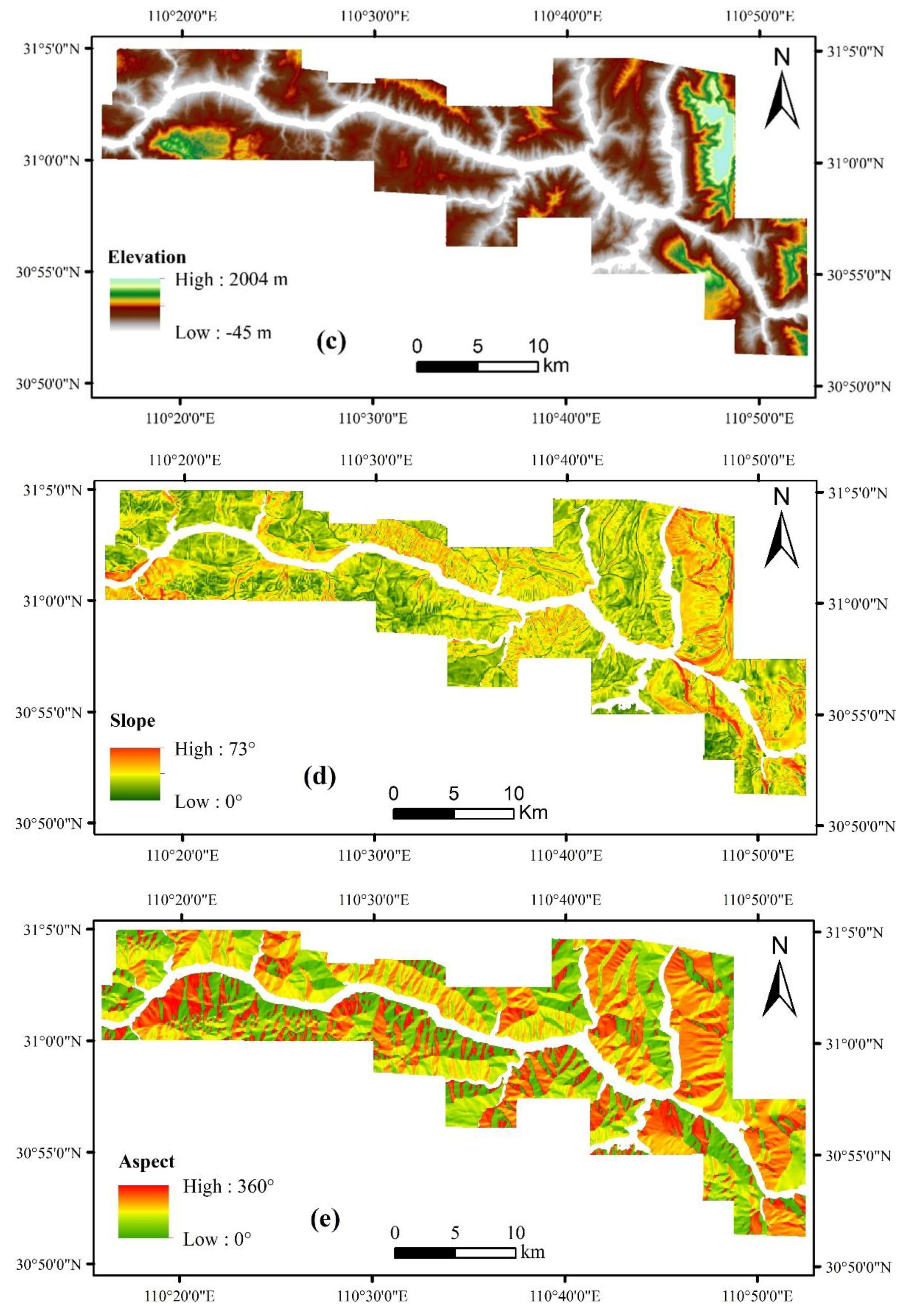
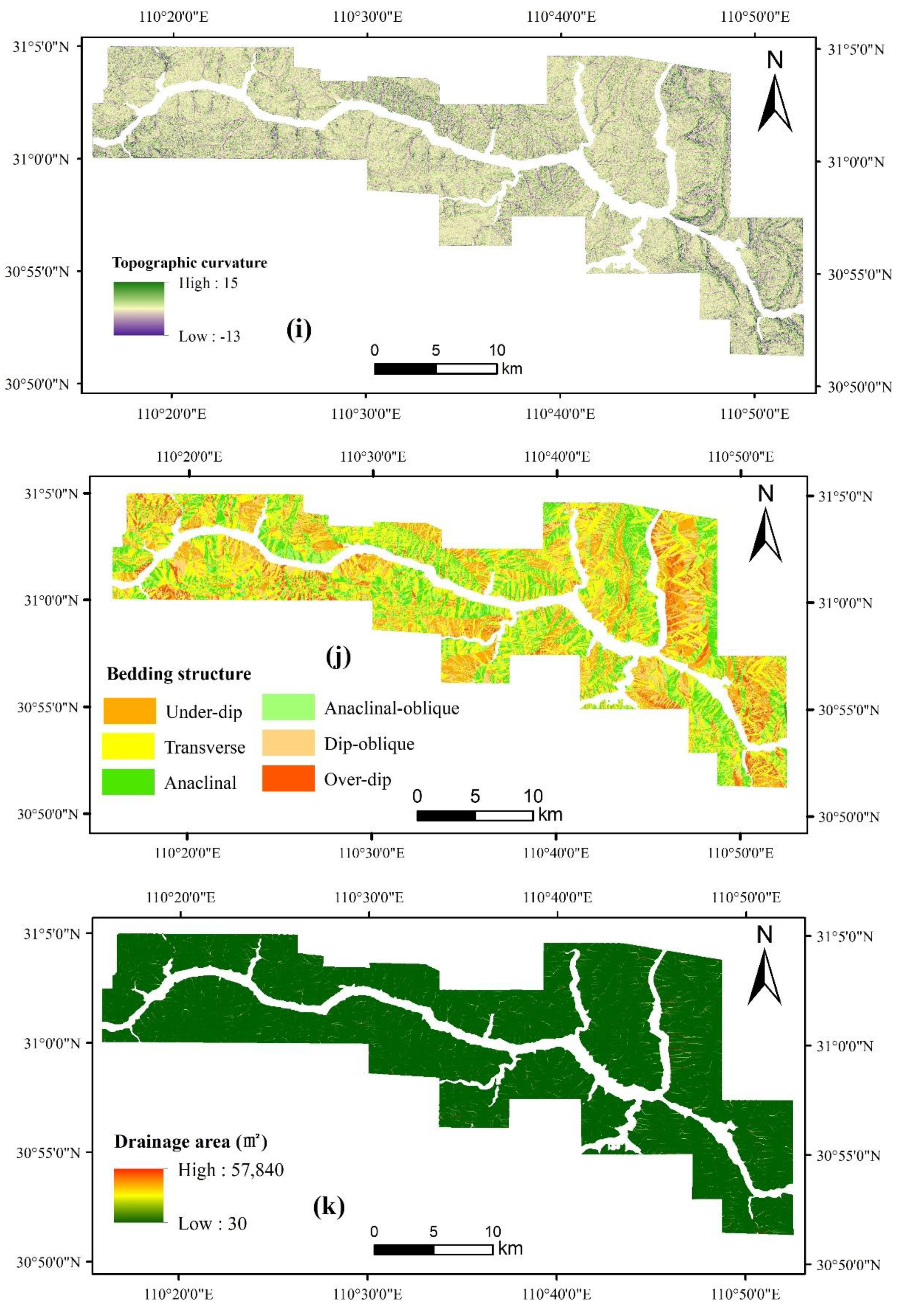
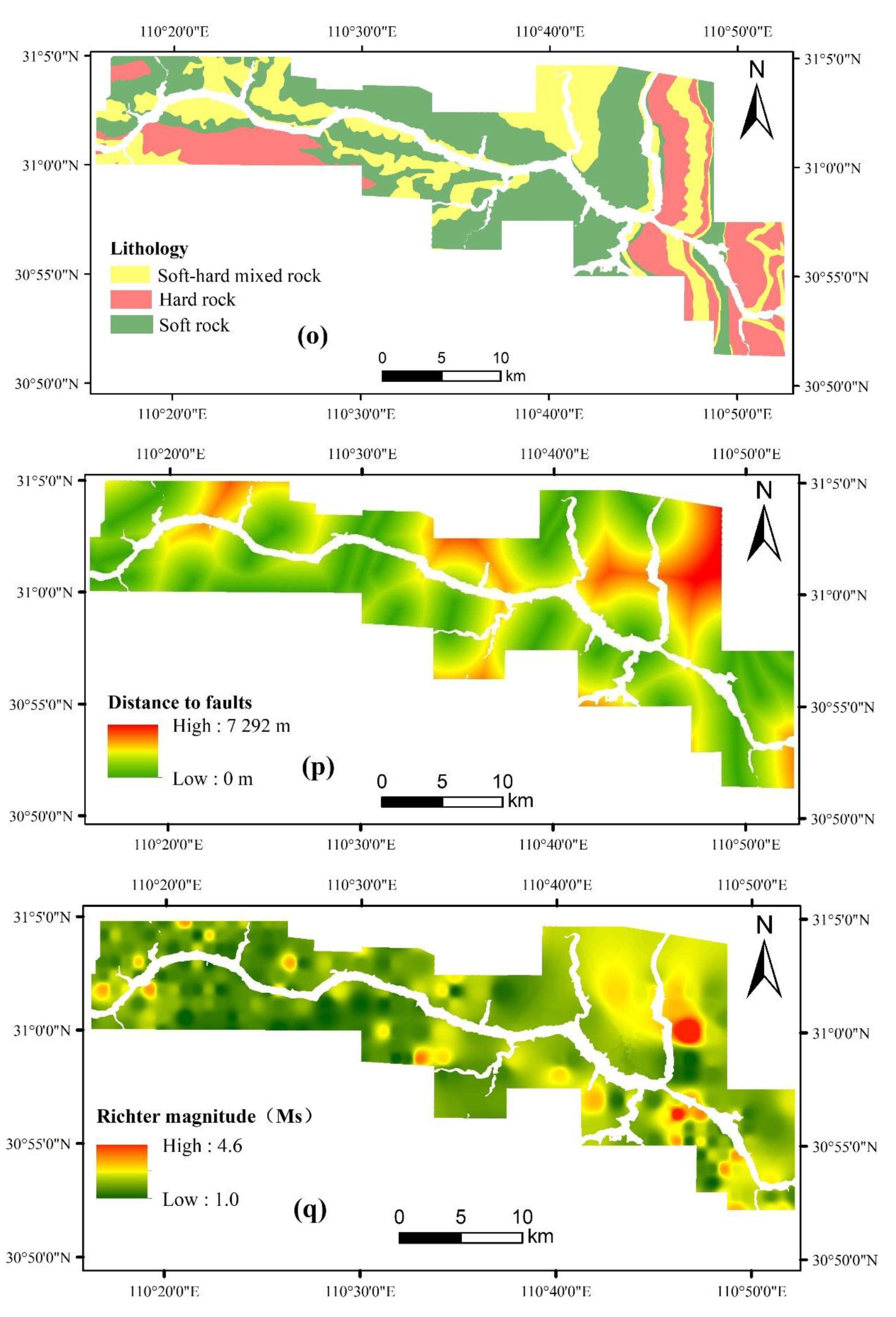
This paper adopted six types of landslide influence factors based on prior research [53,54] and the real situation of the study area. These include land cover, geography, hydrology, geology, earthquakes, and rainfall. The extraction of factors was conducted using GDAL, SAGA, QGIS, and ArcGIS (Table 1).
  • Land cover includes land use and vegetation coverage in this study. Land use is an indicator of the intensity of human activity. In regions where human activities are violent, slope instability rises. Land uses are exacted by pixel classifications from Landsat 8 OLI images and they are then validated by a public dataset [55]. The overall validation accuracy of land use is 89.8%. To make the land use results more reliable, visual interpretation is used to correct misclassifications. Plant roots hold soil and rock in place, and absorb water in the soil at the same time. It usually exerts a positive effect on landslides [56]. The vegetation coverage is computed based on the dimidiate pixel model and normalized difference vegetation index (NDVI).
  • Topography is an essential condition to control the development of landslides [56]. The slope, aspect, slope form, terrain surface texture, terrain ruggedness index, and topographic curvature are derived from the elevation. It must be noted that the bedding structures are a combination of topographic conditions and geological conditions. The bedding structures are classified into six types according to the previous literature [57].
  • Hydrological conditions are also an important factor influencing the occurrence of landslides in the study area [58]. The rivers erode the riverbed on both sides, making the slope unstable. Thus, the landslides in the study area are mainly distributed on both sides of the river. Drainage area, flow path length, stream power index, and distance to rivers are used for LSA modeling.
  • Geological conditions play a decisive role in the development of landslides and are important internal controlling factors. The faults destroy rock formations and affect their stability [59]. The closer to the faults, the greater impact on the rock formation. The geological factors including the lithology and the faults are mainly exacted from geological maps by vectorization.
  • Earthquakes squeeze and stretch the formation, causing huge deformations of the formation and resulting in drastic changes in the geological environment, and finally affect the stability of the slope [60]. The earthquake data were collected from earthquake monitoring sites and then imported into GIS software for further processing.
  • Rainfall affects the water content in the soil and it is one of the main factors that trigger landslides [61,62]. Short-term heavy rainfall may lead to soil erosion, an increase in surface runoff, and a reduction in the soil’s and rock’s absorption capacity. Simultaneously, the rainfall causes fluctuations in reservoir water levels, and the static and dynamic water pressures vary accordingly, aggravating the slope further.
Different factors, regardless of whether the original data source is a raster layer or a vector layer, were converted into 30 × 30 m raster layers eventually. The influence raster layers are shown in Figure 6. The river area is masked from the original layers. The influence factor layers and the landslide inventory layer were aligned and stacked by geographical location in GIS software. It must be noted that each landslide influence factor with continuous values was reclassified into several classes in most of the previous literature [16,63]. However, the continuous landslide influence factors were not reclassified in this study and they were directly fed to the LSA models. Thus, the reclassification processes of factors were performed implicitly by the LSA models.

3.3. Spearman Rank Correlation Coefficient

The Pearson correlation coefficient (PCC) is usually used to measure the linear correlations of different datasets [64]. However, landslide influence factors have intricate nonlinear relationships with each other. To eliminate redundant features and reduce noises, the Spearman rank correlation coefficient (SRCC) is employed to select the influence factors with strong predictive ability in LSA. SRCC can be applied to both continuous factors and discrete factors. The computation of SRCC is similar to the computation of PCC. The difference is that the SRCC calculations use rank factors rather than raw factors [65]. The SRCC is defined as Equation (4).
S R C C X , Y = c o v ( R ( X ) , R ( Y ) ) σ R ( X ) σ R ( Y ) = E [ ( R ( X ) μ R ( X ) ) ( R ( Y ) μ R ( Y ) ) ] σ R ( X ) σ R ( Y )
where the c o v ( R ( X ) , R ( Y ) ) is the covariance of the two variables, the σ R ( X ) and σ R ( Y ) are the standard deviations of the two variables, whereas μ R ( X ) and μ R ( Y ) are the mean values of the two variables. The absolute value of SRCC ranges from 0 to 1, whereas 0 corresponds to a weak linear correlation and 1 corresponds to a strong linear correlation.

3.4. Performance Evaluation

Since the proportion of landslide area was relatively small compared with the whole study area, the landslide susceptibility assessment is a typical class imbalanced classification task. The non-landslide area was much larger than the landslide area. The ratio of non-landslide to landslide in the study area was up to 15:1. Consequently, using the accuracy to evaluate the landslide susceptibility performance would result in the model preferring to identify the samples as non-landslide zones. Non-landslide samples were defined as the negative class, and landslide samples were defined as the positive class. Four types of prediction results were defined for landslide and non-landslide events. TP (true positive) denotes the landslide sample is classified as the landslide, and the prediction is correct. FP (false positive) denotes the non-landslide sample is classified as the landslide, and the prediction is incorrect. TN (true negative) denotes the non-landslide sample is classified as the non-landslide, and the prediction is correct. FN (false negative) denotes the landslide sample is classified as the non-landslide, and the prediction is incorrect.
  • F1-score
R e c a l l = T P T P + F N
P r e c i s i o n = T P T P + F P
F 1 = 2 × P r e c i s i o n × R e c a l l P r e c i s i o n + R e c a l l
Recall is the proportion of correctly predicted landslides relative to the actual landslides (Equation (5) [66]). Precision is the proportion of correctly predicted landslides among all the data predicted as landslides (Equation (6) [66]). The cost caused by the misclassification of landslides is relatively larger than that of the misclassification of non-landslide. Thus, the recall value can be used to measure whether the landslide prediction is comprehensive. However, recall as the evaluation criterion will make the model tend to predict more samples as landslides, resulting in a high false positives rate. The F1-score is the harmonic average of recall and precision to avoid the model being completely inclined to a certain class, as shown in Equation (7) [67]. Therefore, the F1-scores were used as the evaluation criteria for LSA results.
2.
Receiver operating characteristic curve
The x-axis of the receiver operating characteristic curve (ROC) [68] is the false positive rate (FPR), and the y-axis is the true positive rate (TPR). FPR and TPR are defined in Equations (8) and (9), respectively.
F P R = F P F P + T N
T P R = T P T P + F N
When the sample distribution changes, the ROC curve remains stable. Therefore, it is objective to measure the results of landslide susceptibility with dramatic changes in sample distributions. To quantify the ROC curve, the area under curve (AUC) is used to evaluate the performance of the LSA models. The value of AUC ranged from 0 to 1. A high AUC value corresponds to superior model performance, whereas a low AUC value corresponds to inferior model performance. In general, the AUC value of the model was greater than 0.5. The prediction result of the model was worse than that of a random guess when the AUC value was less than 0.5.

3.5. Assessment Units

The common assessment units for LSA can be summarized into three types: raster pixel units, grid units, and slope units [69,70]. In this paper, raster pixel units were chosen as the assessment units. Each raster pixel unit represents a vector [ x 1 , x 2 , , x n ,   y ] , where x i denotes the value of a landslide influence factor and y denotes the target value at a specified pixel, respectively. Since raster layers cannot be fed directly to a model, the combined raster layer (including the influence factor layers and landslide inventory layer) was exported to a two-dimensional table. The conversion process was as follows: (1) Create a polygon and convert it into a raster layer (called L s ) with the same extent as the study area. (2) Convert the L s into a point layer L p . (3) Exact the pixel values of the combined raster layer (called L c ) into the attribute table of the point layer L p . The rows of the attribute table represent landslide samples, and the columns of the attribute table represent different landslide features.

3.6. Factors Standardization

Different factors have different dimensions, and their values vary widely. Some influence factors are discrete values, whereas other influence factors are continuous values. The discrete factors were mapped to numeric values. In order to reduce the impacts of dimensions on model performances, all factors were normalized by Equation (10) [71].
z = x x ¯ σ
where x is the value of the given factor, x ¯ is the mean value of the given factor and σ is the standard deviation of the given factor.

3.7. Class Weighted Strategy

For the class imbalanced problem, the LSA models tended to predict the minority class (non-landslide) as the majority class (non-landslide) to obtain better overall accuracy. This dramatically diminished the reliability of the LSA models. The class-weighted strategy assigns different penalty weights for the majority class and the minority class, respectively [40]. For example, the class weight ratio (non-landslides vs. landslides) of 1:4 means that the penalty intensity for incorrectly predicting landslides is four times higher than that for incorrectly predicting non-landslides. This mechanism can correct the prediction preferences of the LSA model. Since there was a high ratio of non-landslide samples to landslide samples in the study area, two training strategies were employed: (1) A class balanced strategy; that is, the weights of landslides were greater than the weights of non-landslides. A high weight ratio means the model tends to classify more samples as landslide-prone zones. A low weight ratio leads to the number of misclassified landslide samples increasing. In order to find out the best class weight, the weight ratio of landslides to non-landslides was set at a range of 1 to 15. (2) A class imbalanced strategy; that is, the weights of landslide and non-landslide were handled by the model itself. Generally, the weight ratio was 1:1, which indicated the majority class (non-landslide) and the minority class (landslide) had identical class weights. The model tended to predict more samples as non-landslide to achieve better accuracy. However, it was easy to miss detecting some landslide areas. The two training strategies were compared using the evaluation criteria.

3.8. Experiment Setup

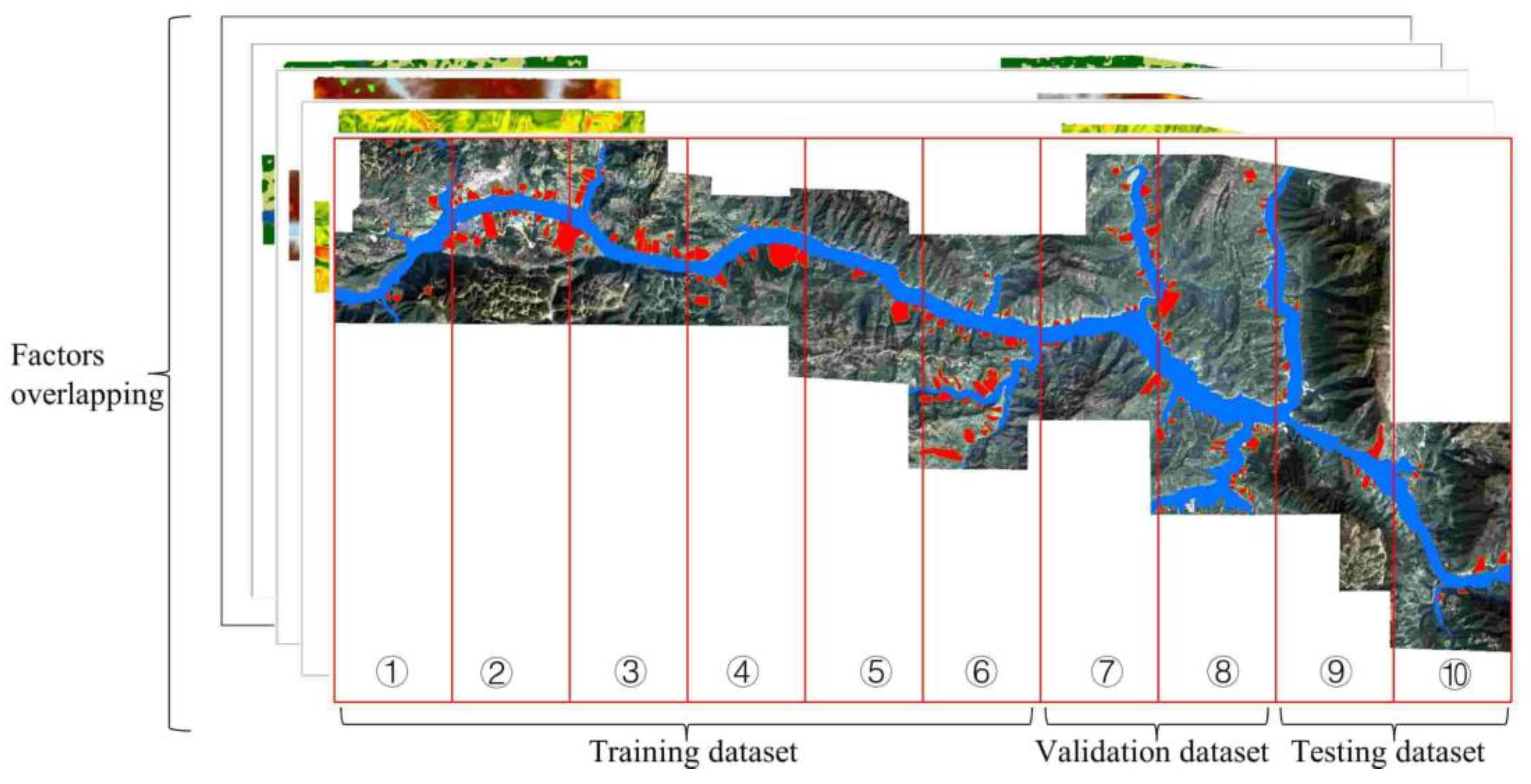
A total of 636,190 pixel-based units were generated and they were used as the entire dataset. The study area was divided into ten parts. Parts 1~6 was the training dataset, parts 7~8 was the validation dataset, and the rest of parts 9 ~10 was the testing dataset (Figure 7). The experiment adopted the class balanced strategy and the class imbalanced strategy. The training device was a personal computer with an AMD 5800 CPU, 32GB of memory, and GeForce RTX3060 12GB GPU. LR and RF were trained on the CPU with parallel settings. For DFCNN and LSTM, the GPU was also used to accelerate the training process. The LR and RF were implemented using the scikit-learn 0.24.2. LR was implemented using LogisticRegression that was built in scikit-learn and newton-cg was used to optimize the algorithm parameters. The maximum iteration of LR was set to 100. RF was implemented using RandomForestClassifier that was built in scikit-learn. Since the distribution of the testing data and the training data may have been quite dissimilar and large tree depths are prone to overfitting, a tiny subset of the study area with significant changes was employed in the pre-testing. The pre-testing results demonstrated that a small tree depth could effectively avoid overfitting and achieve better performances. Thus, the maximum depth of the RF trees was set to 10 based on the outcomes of the preliminary test. The DFCNN was implemented with 4 hidden layers using Keras 2.6.0. Each hidden layer consisted of 8 nodes and was connected to the ReLU activation function. LSTM consisted of 6 LSTM layers and a fully connected layer. The ReLU activation function also was employed for the hidden layer. Both LSTM and DFCNN were trained 200 times.

4. Results

4.1. Performances of Different Class Weights

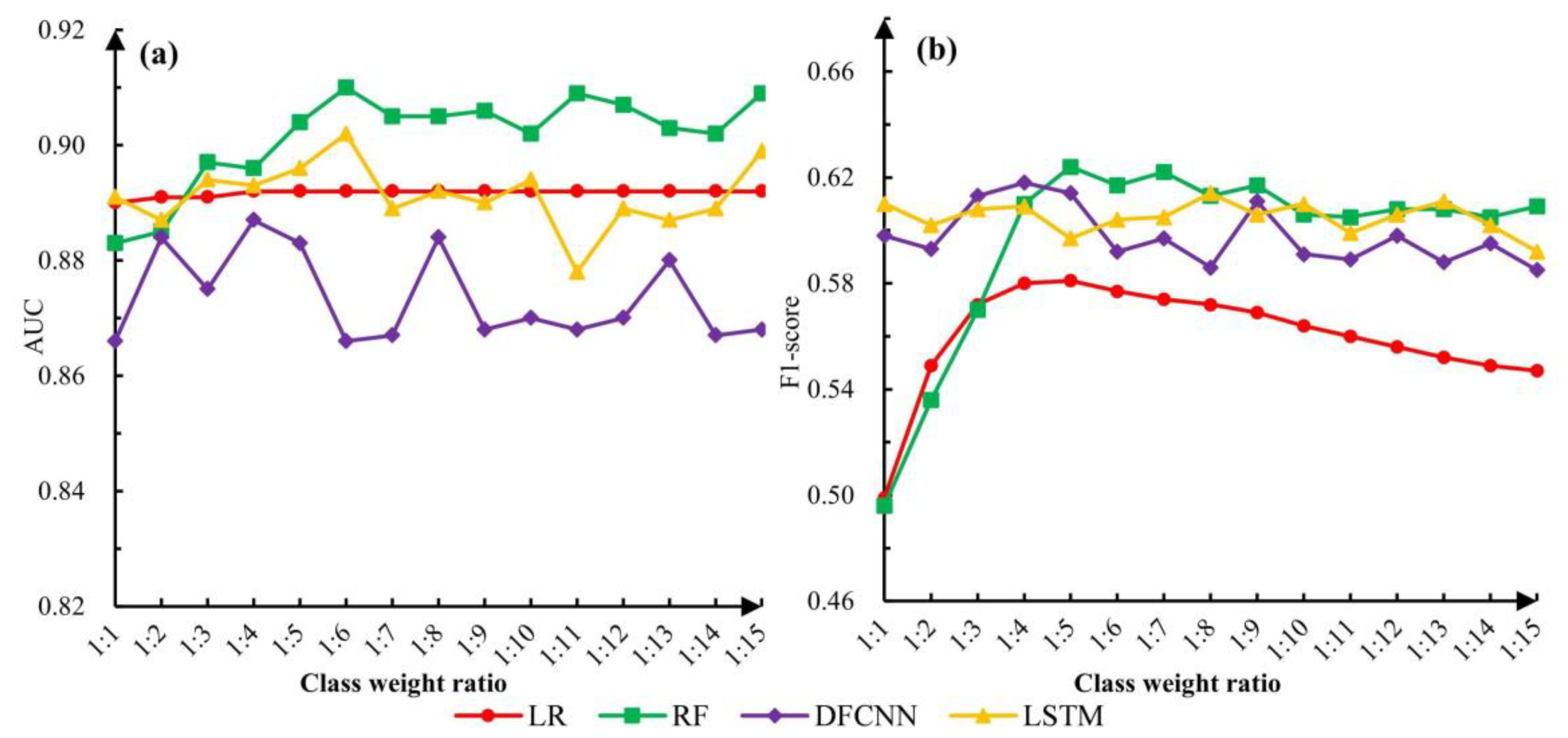
Different class weights lead to changes in model performances. Figure 8 denotes that with the change of class weights, the AUC and F1-score of deep learning models (DFCNN and LSTM) fluctuated without any obvious upward or downward trend. The AUC values of LR remained stable and nearly constant under different class weights. The F1-scores of LR achieved the best performance at class weights of 1:4 and 1:5, and then the performances decreased substantially and gradually. The AUC values of RF fluctuated slightly with different class weights, while F1-scores climbed gradually with increasing class weights, reaching a maximum at class weights of 1:4 and 1:5, and then maintaining small fluctuations. The class weight of 1:4 was chosen to construct the prediction model under the balanced strategy, while the class weight of 1:1 was used to build the prediction model under the imbalanced strategy.

4.2. Correlations of Influence Factors

SRCC was employed to establish the most related landslide influence factors. Figure 9 suggests that the stream power index and the drainage area (SRCC = 0.92), the stream power index and the slope form (SRCC = −0.51), the slope form and the drainage area (SRCC = −0.58), the distance to rivers and the elevation (SRCC = 0.80), the terrain ruggedness index and the slope (SRCC = 0.67), the rainfall and the earthquake magnitude (SRCC = 0.61) were highly correlated, with the absolute SRCC values greater than 0.5. This implies that there may have existed redundant information in these paired landslide influence factors. To explore whether these highly correlated landslide influence factors would affect the performances of the LSA models, these paired influences were first removed separately and then removed simultaneously. Thus, there were 15 scenarios in total, which are shown in Table 2.
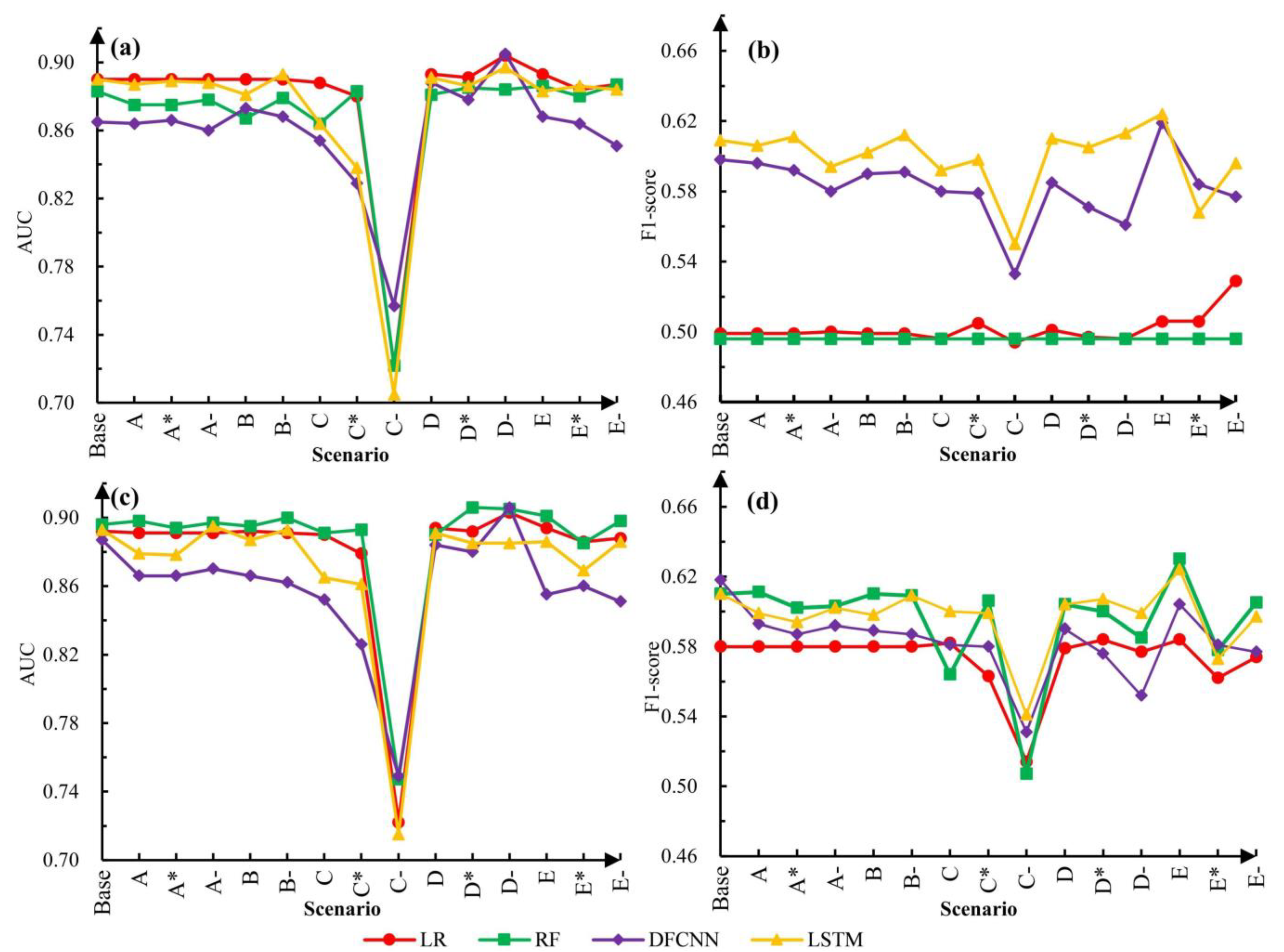
Figure 10 illustrates the performance of these 15 scenarios under a class balanced strategy (class weight ratio is 1:1) and a class imbalanced strategy (class weight ratio is 1:4). In most scenarios, removing some influence factors in the highly correlated factor pairs did not result in significant losses of model performances. However, there were some exceptions. In scenario C-, the AUC values of the four models decreased significantly. Similarly, the F1-scores of four models also dropped dramatically in scenario C-. This demonstrates that the influence factors involved in scenario C- exerted a considerable influence on the occurrence of landslides. They were indispensable in the modeling process.

4.3. Landslide Susceptibility Results

The above experimental results show that the most stable results could be achieved by using the original influence factors. Therefore, the original landslide influence factors were finally used to compare the performances of the four models under the balanced strategy and the imbalanced strategy. Their performances are shown in Table 3. All models achieved high AUC values under two distinct strategies in Figure 11. Therefore, it was not reliable to evaluate the performances of LSA models using the AUC values alone. Under the class imbalanced strategy, the F1-scores of the deep learning models were significantly better than that of the shallow models, while no significant performance differences were observed between the two shallow models. Similarly, no noticeable performance differences were observed between the two deep learning models. Compared with the performances under the class imbalanced strategy, the AUC and F1-score performances of the deep learning models under the class balanced strategy did not change significantly, while the F1-score performances of the shallow models had huge improvements. The improvement of the RF model was more pronounced relative to the LR (up to 0.11).
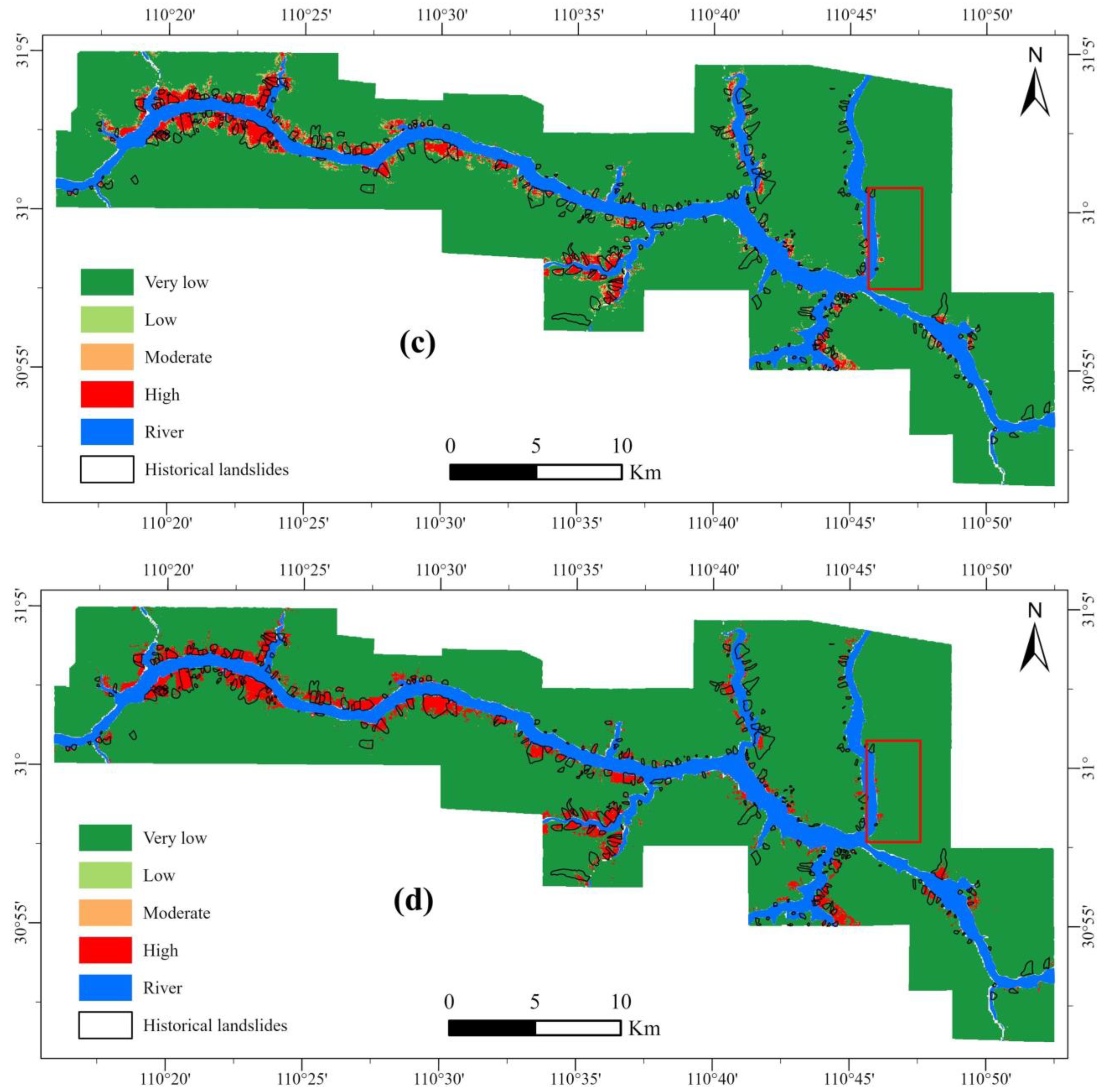
The evaluation results of the models were classified into four susceptibility classes using an equal intervals scheme; namely, very low (<0.25), low (0.25~0.5), moderate (0.5~0.75), and high (>0.75). The experimental results of the four models were connected to the raster pixel unit layer to produce susceptibility images and were compared with historical landslide data for validation. The results of the landslide susceptibility based on the testing dataset are indicated in Figure 12 and Figure 13. The high-risk areas predicted by RF, DFCNN, and LSTM models were distributed on both banks of the river, which is consistent with reality. For the shallow machine learning models, the area of high-risk and moderate-risk regions predicted under the class balanced strategy was significantly higher than those predicted under the class imbalanced strategy. For the deep learning models, the area of high-risk and moderate-risk regions predicted under two different class weighting strategies was nearly identical. Compared with the landslide distribution predicted by deep learning models, the shallow machine learning models predicted wider distributions of landslides and more differentiated hazard hierarchies. It can be found that there was a significant difference in the susceptibility patterns between the deep learning models and shallow machine learning models.

5. Discussion

5.1. Comparison of Performances

Figure 12 demonstrates the high-risk areas predicted by the deep models had a higher overlap with the historical landslides, and this is consistent with those demonstrated by the performance evaluation metrics in Table 3. The AUC values of the shallow models slightly outperformed the deep learning model under the class imbalanced strategy. However, the F1-scores of the deep learning models outperformed the shallow machine learning models by an increase of 0.10 to 0.11. These results have some commonalities with those reported in previous studies. Deep learning models do not always outperform shallow models in AUC performances; this is especially the case with the RF model among the various shallow models, which is reported to be superior to the deep learning models in terms of AUC values in some cases [72]. Meanwhile, the deep learning models generally achieve better F1-score performances compared to the shallow models [73]. Thus, the deep learning models still outperformed shallow models in terms of the overall performances. It is worth mentioning that in previous research, sampling techniques were often used to obtain roughly equal numbers of landslide and non-landslide samples [74]. In this study, no sampling techniques were used and the performances of deep learning models were still similar to those in previous studies. It might be required to investigate the necessity of sampling techniques in deep learning LSA models in the future.
When the class balanced strategy was applied, the F1-scores of LR and RF rose rapidly, which indicates a substantial improvement in predicting high-risk regions. The proportion of moderate-risk predicted by LR increased from 1.57% to 6.81%, and the proportion of high-risk predicted by LR increased from 0.23% to 2.32%. Meanwhile, the proportion of low-risk decreased significantly from 92.10% to 78.26% (Figure 14). Similar trends were observed in the results of the RF. These phenomena verify the effectiveness of the class-weighted strategy for shallow machine learning models. When the class balanced strategy was adopted, the proportion of very low-risk, low-risk, and moderate-risk predicted by DFCNN and LSTM varied slightly and the overall performances of deep learning models were not significantly improved compared with the class imbalanced strategy. This phenomenon reveals that the two deep learning models were more robust to varying class weights than the conventional shallow machine learning methods. This is because deep learning models have more intricate connections between nodes in different layers, which can represent more complex mapping relations, and have stronger anti-interference abilities. However, the deep learning model also has some shortcomings. It is evident that the deep learning model predicted a small area of low-risk zones and moderate-risk zones, and had a weak predictive power for potential landslides, which may lead it to miss detection of landslides and cause problems for disaster management and decision making. Compared with deep learning models, LR and RF had powerful abilities to explore unknown regions while reliably predicting high-risk areas.

5.2. Susceptibility Spatial Patterns

The susceptibility spatial patterns of shallow models (LR and RF) and deep learning models (DFCNN and LSTM) were different. In the cases of deep learning models, high-risk areas were surrounded by pure very low-risk areas, and the proportion of the moderate-risk regions was quite low. However, in the case of shallow models, high-risk areas were surrounded by a much larger proportion of moderate-risk and low-risk areas compared to the deep learning models, and the deep learning models obtained more accurate results in high-risk landslide areas. The results of shallow models had richer hierarchies than deep learning models. This indicates the shallow models are suitable for scenarios requiring hierarchical emergency response. The deep learning models generated more accurate predictions of high-risk landslide areas, which represents that deep learning models are more suitable for scenarios that need precise investigations and specified treatments. However, neither the deep learning models nor the shallow models can completely predicted all landslide zones, and all of these models missed some potentially dangerous landslides. It is worth noting that there were also some regions (red rectangle in Figure 12 and Figure 13) that were predicted as risk zones by two models (LR and RF), but these regions are not marked in the historical landslide survey data. These parts may be future high-risk zones that require some precautions by decision makers.

5.3. Influences of Class Weights

Since LSA is a problem of imbalanced data classification, it is usually considered that class weights can improve the reliability of the evaluation results. Figure 8 illustrates that class weights had a negligible impact on deep learning models. In contrast, class weights had a tremendous impact on the shallow models and can substantially improve the balanced performances between landslides and non-landslides. However, with the class weights increase of the minority class, the F1-score values of the shallow models (LR and RF) first increased and then decreased. This is due to the fact that with the change of class weights, the shallow model can predict landslides more accurately. When a certain limit is exceeded, it leads to a decrease in the performance of the predicted non-landslides, thus reducing the overall performance. It can be concluded that determining the appropriate class weights is critical for shallow models when faced with LSA problems in unknown zones. The optimal class weight reported by [40] differs from this study. This implies that the optimal class weights vary with the dataset and the class weighted strategy usually exerts a positive effect on the shallow machine learning models. Typically, the optimal class weight is determined by conducting numerous tests on existing historical data. However, this way of obtaining the optimal class weights becomes less reliable when the disparities between the known area and the evaluated area are too large. This difficulty is an important reason that prevents the widespread use of class-weighted strategies in LSA. In scenarios where the training data and test data are very different, it is preferable to employ a well-trained deep learning model.

5.4. Model Evaluation and Factors Processing

The AUC value of each model did not vary tremendously under the two strategies. This suggests that AUC is not feasible as a single evaluation metric for LSA models. It is necessary to use multiple model evaluation metrics. We employed the F1-score as the main metric for evaluating the model performances. Nevertheless, high F1-score values prefer to predict more samples as landslide areas, which may raise the cost of landslide prevention. Determining the appropriate F1-score is a tricky problem to be solved, which is related to our practical needs and the cost we are willing to pay to prevent landslides.
Figure 10 illustrates that removing the distance to rivers and elevation greatly affected the performances of the models while removing the distance to rivers or elevation alone did not significantly reduce the performance. This suggests that these two factors are the most critical factors affecting LSA modeling. However, the most important landslide influence factors vary across the literature [19,75,76,77]. It is important to note that various studies in the literature adopt diverse factor analysis methods, which may lead to different key factors being observed. However, even if the same factor analysis method is used, the importance rankings of landslide influence factors observed in different study areas are different [33]. This indicates that there is no constant pattern in the relationship between landslide influence factors and landslide occurrences. Thus, it is necessary to perform factor analysis to select the appropriate landslide influence factor in data-driven LSA modeling. It also reveals that the relationships between influencing factors are complicated, and the joint action of the influence factors affects the final prediction ability of the models.

5.5. Training Time Consumed

The average time consumed by shallow machine learning methods and deep learning methods in the training stage is illustrated in Table 4. The training time required by deep learning models was up to 765 times longer than that required by shallow machine learning models. In the shallow models, RF achieved pretty good performances with a very low time overhead. DFCNN and LSTM achieved the best performances and stable results at the cost of the enormous time overhead. As it is reported in [78], the training time consumed is a necessary consideration when choosing a suitable LSA model. Deep learning models require faster computing devices, and the model building processes are more complicated [33]. Since deep learning models generally require GPUs to accelerate the computation, in the absence of high-performance computing cards, rapid landslide susceptibility mapping cannot be accomplished using deep learning methods. The model structures and hyperparameters need to be fine-tuned in the training stage [22] and these activities are generally not counted in the consumption time. Nevertheless, the time cost of designing network structures and adjusting hyperparameters cannot be ignored in actual disaster prevention. Therefore, RF is still an attractive option to build the LSA model quickly and obtain acceptable prediction results. Deep learning methods are preferable for achieving more consistent results.

6. Conclusions

In this study, eighteen landslide influence factors were selected for landslide susceptibility assessment. LR, RF, DFCNN, and LSTM were employed as the assessment models and their performances were compared. In general, the AUC values of the four models were greater than 0.8 under the class balanced strategy and the class imbalanced strategy, which implies they could be used as credible LSA models. RF performed best in shallow machine learning models, which can balance the training time and the performance. The deep learning models (DFCNN and LSTM) achieved better overall performances and greater robustness than shallow models at the cost of the more significant time overhead. The shallow models were more sensitive to class weights, while the deep learning models were relatively insensitive. It is verified that removing a single or a few landslide influence factors did not substantially affect the accuracy of LSA results except distance to rivers and elevation in this study. The evaluation results of the shallow models had richer landslide susceptibility hierarchies, whereas the deep learning models identified the high-risk landslide zones better. However, whether most shallow machine learning models and deep learning models have the same benefits and drawbacks requires further experimental validation. To ensure the LSA models’ stability across various imbalanced landslide datasets, more robust methods for estimating class weights must be developed in the future.
In conclusion, the class balanced strategy must be adopted when using LR and RF for LSA modeling. The deep learning models (DFCNN and LSTM) have superior adaptability and can be used in an imbalanced dataset. The findings presented in this research can serve as a reference for model selection in LSA and further provide decision support for land management and disaster prevention and mitigation.

Author Contributions

Conceptualization, Y.S. and S.X.; methodology, S.X. and Y.S.; software, S.X.; validation, X.H. and S.X; formal analysis, S.X.; investigation, Y.S.; data curation, S.X. and X.H.; writing—original draft preparation, S.X.; writing—review and editing, Y.S and X.H. All authors have read and agreed to the published version of the manuscript.

Funding

This research was funded by the Zhejiang Province Key Laboratory of Smart Management & Application of Modern Agricultural Resources (Grant No. 2020E10017), Science and Technology Research Project of Jiangxi Provincial Department of Education (Grant No. GJJ200748) and Jiangxi Provincial Natural Science Foundation (Grant No. 20202BAB204035).

Institutional Review Board Statement

Not applicable.

Informed Consent Statement

Not applicable.

Data Availability Statement

The elevation data are available at https://www.earthdata.nasa.gov/ (accessed on 10 June 2021). The Landsat images presented in this study are obtained from USGS earth explorer and they are openly available at https://earthexplorer.usgs.gov/ (accessed on 10 June 2021). Rainfall data are collected from Climate Hazards Group InfraRed Precipitation with Station data at https://data.chc.ucsb.edu/products/CHIRPS-2.0/ (accessed on 3 November 2022). Seismic data and landslide inventory data are available upon request from the corresponding author.

Conflicts of Interest

The authors declare that they have no known competing financial interests or personal relationships that could have appeared to influence the work reported in this paper.

References

  1. Argyriou, A.V.; Teeuw, R.M.; Rust, D.; Sarris, A. GIS multi-criteria decision analysis for assessment and mapping of neotectonic landscape deformation: A case study from Crete. Geomorphology 2016, 253, 262–274. [Google Scholar] [CrossRef] [Green Version]
  2. Vahidnia, M.H.; Alesheikh, A.A.; Alimohammadi, A.; Hosseinali, F. A GIS-based neuro-fuzzy procedure for integrating knowledge and data in landslide susceptibility mapping. Comput. Geosci. 2010, 36, 1101–1114. [Google Scholar] [CrossRef]
  3. Cabral, V.C.; Reis, F.A.G.V. Assessment of Shallow Landslides Susceptibility Using SHALSTAB and SINMAP at Serra Do Mar, Brazil. In Understanding and Reducing Landslide Disaster Risk; Guzzetti, F., Mihalić Arbanas, S., Reichenbach, P., Sassa, K., Bobrowsky, P.T., Takara, K., Eds.; Springer: Cham, Switzerland, 2021; Volume 2, pp. 257–265. [Google Scholar] [CrossRef]
  4. Fernandes, N.F.; Guimarães, R.F.; Gomes, R.A.T.; Vieira, B.C.; Montgomery, D.R.; Greenberg, H. Topographic controls of landslides in Rio de Janeiro: Field evidence and modeling. Catena 2004, 55, 163–181. [Google Scholar] [CrossRef]
  5. Ciurleo, M.; Cascini, L.; Calvello, M. A comparison of statistical and deterministic methods for shallow landslide susceptibility zoning in clayey soils. Eng. Geol. 2017, 223, 71–81. [Google Scholar] [CrossRef]
  6. Lin, W.; Yin, K.; Wang, N.; Xu, Y.; Guo, Z.; Li, Y. Landslide hazard assessment of rainfall-induced landslide based on the CF-SINMAP model: A case study from Wuling Mountain in Hunan Province, China. Nat. Hazards 2021, 106, 679–700. [Google Scholar] [CrossRef]
  7. Melo, C.M.; Kobiyama, M.; Michel, G.P.; de Brito, M.M. The Relevance of Geotechnical-Unit Characterization for Landslide-Susceptibility Mapping with SHALSTAB. GeoHazards 2021, 2, 383–397. [Google Scholar] [CrossRef]
  8. Chen, W.; Li, W.; Chai, H.; Hou, E.; Li, X.; Ding, X. GIS-based landslide susceptibility mapping using analytical hierarchy process (AHP) and certainty factor (CF) models for the Baozhong region of Baoji City, China. Environ. Earth Sci. 2016, 75, 1–14. [Google Scholar] [CrossRef]
  9. Vilasan, R.T.; Kapse, V.S. Evaluation of the prediction capability of AHP and F-AHP methods in flood susceptibility mapping of Ernakulam district (India). Nat. Hazards 2022, 112, 1767–1793. [Google Scholar] [CrossRef]
  10. Merghadi, A.; Yunus, A.P.; Dou, J.; Whiteley, J.; ThaiPham, B.; Bui, D.T.; Avtar, R.; Abderrahmane, B. Machine learning methods for landslide susceptibility studies: A comparative overview of algorithm performance. Earth-Sci. Rev. 2020, 207, 103225. [Google Scholar] [CrossRef]
  11. Wang, L.; Guo, M.; Sawada, K.; Lin, J.; Zhang, J. A comparative study of landslide susceptibility maps using logistic regression, frequency ratio, decision tree, weights of evidence and artificial neural network. Geosci. J. 2016, 20, 117–136. [Google Scholar] [CrossRef]
  12. Wang, Q.; Wang, Y.; Niu, R.; Peng, L. Integration of Information Theory, K-Means Cluster Analysis and the Logistic Regression Model for Landslide Susceptibility Mapping in the Three Gorges Area, China. Remote Sens. 2017, 9, 938. [Google Scholar] [CrossRef] [Green Version]
  13. Zhou, X.; Wu, W.; Qin, Y.; Fu, X. Geoinformation-based landslide susceptibility mapping in subtropical area. Sci. Rep. 2021, 11, 1–16. [Google Scholar] [CrossRef] [PubMed]
  14. Yu, X.; Wang, Y.; Niu, R.; Hu, Y. A Combination of Geographically Weighted Regression, Particle Swarm Optimization and Support Vector Machine for Landslide Susceptibility Mapping: A Case Study at Wanzhou in the Three Gorges Area, China. Int. J. Environ. Res. Public Health 2016, 13, 487. [Google Scholar] [CrossRef] [PubMed] [Green Version]
  15. Kainthura, P.; Sharma, N. Machine learning driven landslide susceptibility prediction for the Uttarkashi region of Uttarakhand in India. Georisk Assess. Manag. Risk Eng. Syst. Geohazards 2021, 16, 570–583. [Google Scholar] [CrossRef]
  16. Chen, W.; Xie, X.; Wang, J.; Pradhan, B.; Hong, H.; Bui, D.T.; Duan, Z.; Ma, J. A comparative study of logistic model tree, random forest, and classification and regression tree models for spatial prediction of landslide susceptibility. Catena 2017, 151, 147–160. [Google Scholar] [CrossRef] [Green Version]
  17. Zhou, X.; Wen, H.; Zhang, Y.; Xu, J.; Zhang, W. Landslide susceptibility mapping using hybrid random forest with GeoDetector and RFE for factor optimization. Geosci. Front. 2021, 12, 101211. [Google Scholar] [CrossRef]
  18. Dou, J.; Yamagishi, H.; Pourghasemi, H.R.; Yunus, A.P.; Song, X.; Xu, Y.; Zhu, Z. An integrated artificial neural network model for the landslide susceptibility assessment of Osado Island, Japan. Nat. Hazards 2015, 78, 1749–1776. [Google Scholar] [CrossRef]
  19. Pham, B.T.; Van Dao, D.; Acharya, T.D.; Van Phong, T.; Costache, R.; Van Le, H.; Nguyen, H.B.T.; Prakash, I. Performance assessment of artificial neural network using chi-square and backward elimination feature selection methods for landslide susceptibility analysis. Environ. Earth Sci. 2021, 80, 686. [Google Scholar] [CrossRef]
  20. Zhou, X.; Wen, H.; Li, Z.; Zhang, H.; Zhang, W. An interpretable model for the susceptibility of rainfall-induced shallow landslides based on SHAP and XGBoost. Geocarto Int. 2022, 1–32. [Google Scholar] [CrossRef]
  21. Saha, S.; Roy, J.; Pradhan, B.; Hembram, T.K. Hybrid ensemble machine learning approaches for landslide susceptibility mapping using different sampling ratios at East Sikkim Himalayan, India. Adv. Space Res. 2021, 68, 2819–2840. [Google Scholar] [CrossRef]
  22. Bui, D.T.; Tsangaratos, P.; Nguyen, V.; Liem, N.V.; Trinh, P.T. Comparing the prediction performance of a Deep Learning Neural Network model with conventional machine learning models in landslide susceptibility assessment. Catena 2020, 188, 104426. [Google Scholar] [CrossRef]
  23. Sun, D.; Gu, Q.; Wen, H.; Shi, S.; Mi, C.; Zhang, F. A Hybrid Landslide Warning Model Coupling Susceptibility Zoning and Precipitation. Forests 2022, 13, 827. [Google Scholar] [CrossRef]
  24. Zhang, W.; Liu, S.; Wang, L.; Samui, P.; Chwała, M.; He, Y. Landslide Susceptibility Research Combining Qualitative Analysis and Quantitative Evaluation: A Case Study of Yunyang County in Chongqing, China. Forests 2022, 13, 1055. [Google Scholar] [CrossRef]
  25. Chai, J.; Zeng, H.; Li, A.; Ngai, E.W.T. Deep learning in computer vision: A critical review of emerging techniques and application scenarios. Mach. Learn. Appl. 2021, 6, 100134. [Google Scholar] [CrossRef]
  26. Otter, D.W.; Medina, J.R.; Kalita, J.K. A Survey of the Usages of Deep Learning for Natural Language Processing. IEEE Trans. Neural Netw. Learn. Syst. 2021, 32, 604–624. [Google Scholar] [CrossRef] [Green Version]
  27. Grigorescu, S.; Trasnea, B.; Cocias, T.; Macesanu, G. A survey of deep learning techniques for autonomous driving. J. Field Robot. 2020, 37, 362–386. [Google Scholar] [CrossRef] [Green Version]
  28. Esteva, A.; Chou, K.; Yeung, S.; Naik, N.; Madani, A.; Mottaghi, A.; Liu, Y.; Topol, E.; Dean, J.; Socher, R. Deep learning-enabled medical computer vision. NPJ Digit. Med. 2021, 4, 5. [Google Scholar] [CrossRef] [PubMed]
  29. Bera, S.; Upadhyay, V.K.; Guru, B.; Oommen, T. Landslide inventory and susceptibility models considering the landslide typology using deep learning: Himalayas, India. Nat. Hazards 2021, 108, 1257–1289. [Google Scholar] [CrossRef]
  30. Thi Ngo, P.T.; Panahi, M.; Khosravi, K.; Ghorbanzadeh, O.; Kariminejad, N.; Cerda, A.; Lee, S. Evaluation of deep learning algorithms for national scale landslide susceptibility mapping of Iran. Geosci. Front. 2021, 12, 505–519. [Google Scholar] [CrossRef]
  31. Wang, H.; Zhang, L.; Luo, H.; He, J.; Cheung, R.W.M. AI-powered landslide susceptibility assessment in Hong Kong. Eng. Geol. 2021, 288, 106103. [Google Scholar] [CrossRef]
  32. Wang, W.; He, Z.; Han, Z.; Li, Y.; Dou, J.; Huang, J. Mapping the susceptibility to landslides based on the deep belief network: A case study in Sichuan Province, China. Nat. Hazards 2020, 103, 3239–3261. [Google Scholar] [CrossRef]
  33. Liu, R.; Yang, X.; Xu, C.; Wei, L.; Zeng, X. Comparative Study of Convolutional Neural Network and Conventional Machine Learning Methods for Landslide Susceptibility Mapping. Remote Sens. 2022, 14, 321. [Google Scholar] [CrossRef]
  34. Azarafza, M.; Azarafza, M.; Akgün, H.; Atkinson, P.M.; Derakhshani, R. Deep learning-based landslide susceptibility mapping. Sci. Rep. 2021, 11, 24112. [Google Scholar] [CrossRef] [PubMed]
  35. Yi, Y.; Zhang, Z.; Zhang, W.; Jia, H.; Zhang, J. Landslide susceptibility mapping using multiscale sampling strategy and convolutional neural network: A case study in Jiuzhaigou region. Catena 2020, 195, 104851. [Google Scholar] [CrossRef]
  36. Sameen, M.I.; Pradhan, B.; Lee, S. Application of convolutional neural networks featuring Bayesian optimization for landslide susceptibility assessment. Catena 2020, 186, 104249. [Google Scholar] [CrossRef]
  37. Habumugisha, J.M.; Chen, N.; Rahman, M.; Islam, M.M.; Ahmad, H.; Elbeltagi, A.; Sharma, G.; Liza, S.N.; Dewan, A.M. Landslide Susceptibility Mapping with Deep Learning Algorithms. Sustainability 2022, 14, 1734. [Google Scholar] [CrossRef]
  38. Wu, B.; Qiu, W.; Jia, J.; Liu, N. Landslide Susceptibility Modeling Using Bagging-Based Positive-Unlabeled Learning. IEEE Geosci. Remote Sens. Lett. 2021, 18, 766–770. [Google Scholar] [CrossRef]
  39. Yao, J.; Qin, S.; Qiao, S.; Liu, X.; Zhang, L.; Chen, J. Application of a two-step sampling strategy based on deep neural network for landslide susceptibility mapping. Bull. Eng. Geol. Environ. 2022, 81, 148. [Google Scholar] [CrossRef]
  40. Zhang, H.; Song, Y.; Xu, S.; He, Y.; Li, Z.; Yu, X.; Liang, Y.; Wu, W.; Wang, Y. Combining a class-weighted algorithm and machine learning models in landslide susceptibility mapping: A case study of Wanzhou section of the Three Gorges Reservoir, China. Comput. Geosci. 2022, 158, 104966. [Google Scholar] [CrossRef]
  41. Süzen, M.L.; Kaya, B.Ş. Evaluation of environmental parameters in logistic regression models for landslide susceptibility mapping. Int. J. Digit. Earth 2012, 5, 338–355. [Google Scholar] [CrossRef]
  42. Zhang, M.; Cao, X.; Peng, L.; Niu, R. Landslide susceptibility mapping based on global and local logistic regression models in Three Gorges Reservoir area, China. Environ. Earth Sci. 2016, 75, 958. [Google Scholar] [CrossRef]
  43. Akinci, H.; Zeybek, M. Comparing classical statistic and machine learning models in landslide susceptibility mapping in Ardanuc (Artvin), Turkey. Nat. Hazards 2021, 108, 1515–1543. [Google Scholar] [CrossRef]
  44. Mira, J.; Sandoval, F. From Natural to Artificial Neural Computation: International Workshop on Artificial Neural Networks, Malaga-Torremolinos, Spain, 7–9 June 1995: Proceedings; Springer-Verlag: New York, USA, 1995; Volume 930, pp. 195–201. [Google Scholar]
  45. Chen, W.; Sun, Z.; Zhao, X.; Lei, X.; Shirzadi, A.; Shahabi, H. Performance Evaluation and Comparison of Bivariate Statistical-Based Artificial Intelligence Algorithms for Spatial Prediction of Landslides. ISPRS Int. J. Geo-Inf. 2020, 9, 696. [Google Scholar] [CrossRef]
  46. Akinci, H.; Kilicoglu, C.; Dogan, S. Random Forest-Based Landslide Susceptibility Mapping in Coastal Regions of Artvin, Turkey. ISPRS Int. J. Geo-Inf. 2020, 9, 553. [Google Scholar] [CrossRef]
  47. Akinci, H. Assessment of rainfall-induced landslide susceptibility in Artvin, Turkey using machine learning techniques. J. Afr. Earth Sci. 2022, 191, 104535. [Google Scholar] [CrossRef]
  48. Li, J.; Cheng, J.; Shi, J.; Huang, F. Brief Introduction of Back Propagation (BP) Neural Network Algorithm and Its Improvement. In Advances in Intelligent and Soft Computing, Proceedings of the Advances in Computer Science and Information Engineering; Jin, D., Lin, S., Eds.; Springer-Verlag: Berlin/Heidelberg, Germany, 2012; Volume 169, pp. 553–558. [Google Scholar]
  49. Wang, S.-C. Artificial Neural Network. In Interdisciplinary Computing in Java Programming; Wang, S.-C., Ed.; The Springer International Series in Engineering and Computer Science; Springer US: Boston, MA, USA, 2003; Volume 743, pp. 81–100. [Google Scholar]
  50. Nair, V.; Hinton, G.E. Rectified Linear Units Improve Restricted Boltzmann Machines. In Proceedings of the 27th International Conference on Machine Learning, Haifa, Israel, 21–24 June 2010; ICML: Haifa, Israel, 2010; pp. 807–814. [Google Scholar]
  51. Hochreiter, S.; Schmidhuber, J. Long short-term memory. Neural Comput. 1997, 9, 1735–1780. [Google Scholar] [CrossRef]
  52. Wang, Y.; Fang, Z.; Wang, M.; Peng, L.; Hong, H. Comparative study of landslide susceptibility mapping with different recurrent neural networks. Comput. Geosci. 2020, 138, 104445. [Google Scholar] [CrossRef]
  53. Moosavi, V.; Niazi, Y. Development of hybrid wavelet packet-statistical models (WP-SM) for landslide susceptibility mapping. Landslides 2016, 13, 97–114. [Google Scholar] [CrossRef]
  54. Zhao, C.; Chen, W.; Wang, Q.; Wu, Y.; Yang, B. A comparative study of statistical index and certainty factor models in landslide susceptibility mapping: A case study for the Shangzhou District, Shaanxi Province, China. Arab. J. Geosci. 2015, 8, 9079–9088. [Google Scholar] [CrossRef]
  55. Yang, J.; Huang, X. The 30 m annual land cover dataset and its dynamics in China from 1990 to 2019. Earth Syst. Sci. Data 2021, 13, 3907–3925. [Google Scholar] [CrossRef]
  56. Bourenane, H.; Bouhadad, Y.; Guettouche, M.S.; Braham, M. GIS-based landslide susceptibility zonation using bivariate statistical and expert approaches in the city of Constantine (Northeast Algeria). Bull. Eng. Geol. Environ. 2015, 74, 337–355. [Google Scholar] [CrossRef]
  57. Peng, L.; Niu, R.; Huang, B.; Wu, X.; Zhao, Y.; Ye, R. Landslide susceptibility mapping based on rough set theory and support vector machines: A case of the Three Gorges area, China. Geomorphology 2014, 204, 287–301. [Google Scholar] [CrossRef]
  58. Pourghasemi, H.R.; Rahmati, O. Prediction of the landslide susceptibility: Which algorithm, which precision? Catena 2018, 162, 177–192. [Google Scholar] [CrossRef]
  59. Regmi, N.R.; Giardino, J.R.; McDonald, E.V.; Vitek, J.D. A comparison of logistic regression-based models of susceptibility to landslides in western Colorado, USA. Landslides 2014, 11, 247–262. [Google Scholar] [CrossRef]
  60. Tang, C.; Ma, G.; Chang, M.; Li, W.; Zhang, D.; Jia, T.; Zhou, Z. Landslides triggered by the 20 April 2013 Lushan earthquake, Sichuan Province, China. Eng. Geol. 2015, 187, 45–55. [Google Scholar] [CrossRef]
  61. Fang, Z.; Wang, Y.; Peng, L.; Hong, H. Integration of convolutional neural network and conventional machine learning classifiers for landslide susceptibility mapping. Comput. Geosci. 2020, 139, 104470. [Google Scholar] [CrossRef]
  62. Melillo, M.; Brunetti, M.T.; Peruccacci, S.; Gariano, S.L.; Guzzetti, F. Rainfall thresholds for the possible landslide occurrence in Sicily (Southern Italy) based on the automatic reconstruction of rainfall events. Landslides 2016, 13, 165–172. [Google Scholar] [CrossRef]
  63. Fallah-Zazuli, M.; Vafaeinejad, A.; Alesheykh, A.A.; Modiri, M.; Aghamohammadi, H. Mapping landslide susceptibility in the Zagros Mountains, Iran: A comparative study of different data mining models. Earth Sci. Inform. 2019, 12, 615–628. [Google Scholar] [CrossRef]
  64. Rodgers, J.L.; Nicewander, W.A. Thirteen Ways to Look at the Correlation Coefficient. Am. Stat. 1988, 42, 59–66. [Google Scholar] [CrossRef]
  65. Gauthier, T. Detecting Trends Using Spearman’s Rank Correlation Coefficient. Environ. Forensics 2001, 2, 359–362. [Google Scholar] [CrossRef]
  66. Yu, X.; Zhang, K.; Song, Y.; Jiang, W.; Zhou, J. Study on landslide susceptibility mapping based on rock–soil characteristic factors. Sci. Rep. 2021, 11, 15476. [Google Scholar] [CrossRef] [PubMed]
  67. Flach, P.; Kull, M. Precision-recall-gain curves: PR analysis done right. In Advances in Neural Information Processing Systems; MIT Press: Cambridge, MA, USA, 2015; Volume 1, pp. 838–846. [Google Scholar]
  68. Pontius, R.G.; Parmentier, B. Recommendations for using the relative operating characteristic (ROC). Landsc. Ecol. 2014, 29, 367–382. [Google Scholar] [CrossRef]
  69. Erener, A.; Düzgün, H.S.B. Landslide susceptibility assessment: What are the effects of mapping unit and mapping method? Environ. Earth Sci. 2012, 66, 859–877. [Google Scholar] [CrossRef]
  70. Hussin, H.Y.; Zumpano, V.; Reichenbach, P.; Sterlacchini, S.; Micu, M.; van Westen, C.; Bălteanu, D. Different landslide sampling strategies in a grid-based bi-variate statistical susceptibility model. Geomorphology 2016, 253, 508–523. [Google Scholar] [CrossRef]
  71. Spiegel, M.R.; Schiller, J.J.; Srinivasan, R.A. Schaum’s Outline of Probability and Statistics, 4th ed.; McGraw-Hill Education: Los Angeles, CA, USA, 2013; pp. 75–107. [Google Scholar]
  72. Wang, H.; Zhang, L.; Yin, K.; Luo, H.; Li, J. Landslide identification using machine learning. Geosci. Front. 2021, 12, 351–364. [Google Scholar] [CrossRef]
  73. Xiong, Y.; Zhou, Y.; Wang, F.; Wang, S.; Wang, Z.; Ji, J.; Wang, J.; Zou, W.; You, D.; Qin, G. A Novel Intelligent Method Based on the Gaussian Heatmap Sampling Technique and Convolutional Neural Network for Landslide Susceptibility Mapping. Remote Sens. 2022, 14, 2866. [Google Scholar] [CrossRef]
  74. Fang, Z.; Wang, Y.; Duan, G.; Peng, L. Landslide Susceptibility Mapping Using Rotation Forest Ensemble Technique with Different Decision Trees in the Three Gorges Reservoir Area, China. Remote Sens. 2021, 13, 238. [Google Scholar] [CrossRef]
  75. Wang, Y.; Song, C.; Lin, Q.; Li, J. Occurrence probability assessment of earthquake-triggered landslides with Newmark displacement values and logistic regression: The Wenchuan earthquake, China. Geomorphology 2016, 258, 108–119. [Google Scholar] [CrossRef]
  76. Pineda, M.C.; Viloria, J.; Martínez-Casasnovas, J.A. Landslides susceptibility change over time according to terrain conditions in a mountain area of the tropic region. Environ. Monit. Assess. 2016, 188, 255. [Google Scholar] [CrossRef]
  77. Hua, Y.; Wang, X.; Li, Y.; Xu, P.; Xia, W. Dynamic development of landslide susceptibility based on slope unit and deep neural networks. Landslides 2021, 18, 281–302. [Google Scholar] [CrossRef]
  78. Dao, D.V.; Jaafari, A.; Bayat, M.; Mafi-Gholami, D.; Qi, C.; Moayedi, H.; Phong, T.V.; Ly, H.; Le, T.; Trinh, P.T.; et al. A spatially explicit deep learning neural network model for the prediction of landslide susceptibility. Catena 2020, 188, 104451. [Google Scholar] [CrossRef]
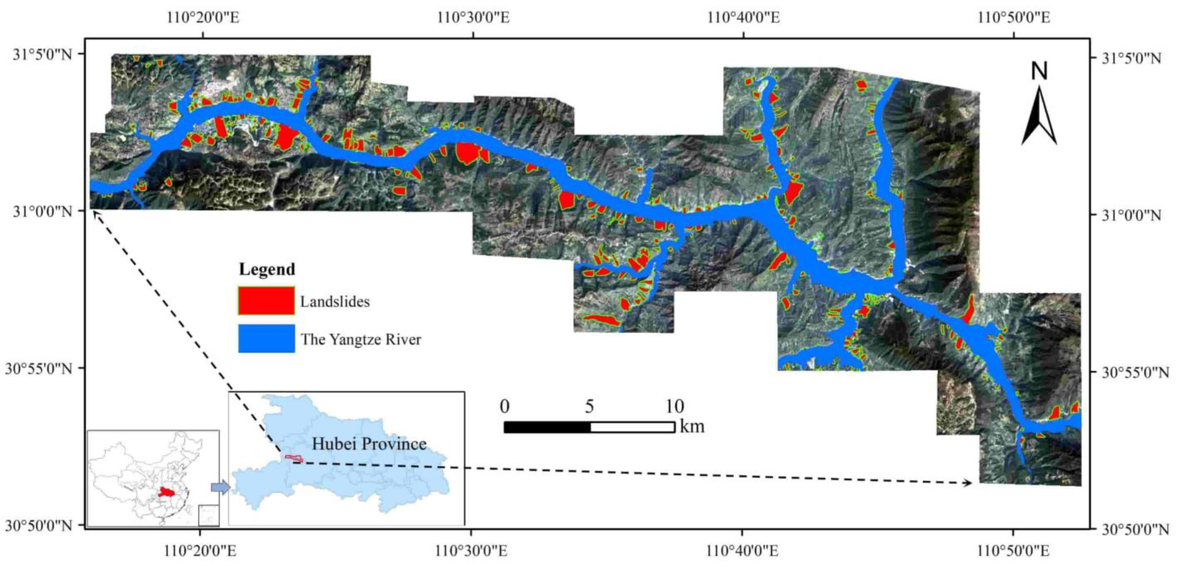
Figure 1. Location of the study area and the landslides’ distribution.
Forests 13 01908 g001
Figure 2. Geological map of the study area.
Forests 13 01908 g002
Figure 3. Methodological flowchart of the study.
Forests 13 01908 g003
Figure 4. Architecture of DFCNN.
Forests 13 01908 g004
Figure 5. Architecture of the memory block at time step t.
Forests 13 01908 g005
Figure 6. Landslide influence factors: (a) vegetation coverage, (b) land use, (c) elevation, (d) slope, (e) aspect, (f) slope form, (g) terrain surface texture, (h) terrain ruggedness index, (i) topographic curvature, (j) bedding structure, (k) drainage area, (l) flow path length, (m) stream power index, (n) distance to rivers, (o) lithology, (p) distance to faults, (q) earthquake magnitude, (r) rainfall.
Forests 13 01908 g006aForests 13 01908 g006bForests 13 01908 g006cForests 13 01908 g006dForests 13 01908 g006eForests 13 01908 g006fForests 13 01908 g006g
Figure 7. Diagram of dataset splitting.
Forests 13 01908 g007
Figure 8. Performances with different class weight ratios: (a) AUC performances, (b) F1-score performances.
Forests 13 01908 g008
Figure 9. SRCC between landslide influence factors and the landslides.
Forests 13 01908 g009
Figure 10. Performances of removing landslide influence factors: (a) AUC under class imbalanced strategy, (b) F1-score under class imbalanced strategy, (c) AUC under class balanced strategy, (d) F1-score under class balanced strategy.
Forests 13 01908 g010
Figure 11. ROC curves of four models: (a) ROC curves under class imbalanced strategy, (b) ROC curves under class balanced strategy.
Forests 13 01908 g011
Figure 12. LSA results under the class imbalanced strategy: (a) result of LR, (b) result of RF, (c) result of DFCNN, (d) result of LSTM.
Forests 13 01908 g012aForests 13 01908 g012b
Figure 13. LSA results under the class balanced strategy: (a) result of LR, (b) result of RF, (c) result of DFCNN, (d) result of LSTM.
Forests 13 01908 g013aForests 13 01908 g013b
Figure 14. Proportions of different landslide risk levels of four models: (a) class imbalanced strategy, (b) class balanced strategy.
Forests 13 01908 g014
Table 1. Landslide influence factors, the exaction tools used, and their variable types.
Data SourceTypeExaction ToolsVariable TypeInfluence Factor
Landsat imagesLand coverPreprocessing, vegetation coverage estimation based on dimidiate pixel models, and implemented using python in ArcGISContinuousVegetation coverage
Preprocessing, pixel classification in QGISDiscreteLand use
DEMTopographyDirect utilizationContinuousElevation
Model calculation based on the terrain analysis tool of GDALContinuousSlope
Model calculation based on the terrain analysis tool of GDALContinuousAspect
Model calculation using curvature tools of SAGADiscreteSlope form
Model calculation using the terrain analysis tool of SAGAContinuousTerrain surface texture
Model calculation using the terrain analysis tool of SAGAContinuousTerrain ruggedness index
Model calculation using curvature tools of SAGAContinuousTopographic curvature
Vectorization, rasterization, and calculation based on slope and aspect in QGISDiscreteBedding structure
DEM
Landsat image
HydrologicalModel calculation using terrain analysis—hydrology tool of SAGAContinuousDrainage area
Model calculation using terrain analysis—hydrology tool of SAGAContinuousFlow path length
Model calculation using terrain analysis—hydrology tool of SAGAContinuousStream power index
Model calculation based on proximity (Raster distance) tool of QGISContinuousDistance to rivers
Geological mapGeologicalVectorization, rasterization, and reclassifying in QGISDiscreteLithology
Vectorization, rasterization, and model calculation based on the proximity (raster distance) tool of QGISContinuousDistance to faults
Earthquake monitoring sitesEarthquakeModel calculation using TIN interpolation in QGISContinuousEarthquake magnitude
Rainfall dataRainfallDirect utilizationContinuousRainfall
Table 2. Scenarios of removing highly correlated influence factors.
ScenarioInfluence Factors Removed
BaseAll factors are used
AStream power index
A*Drainage area
A-Stream power index, drainage area
BSlope form
B-Slope form, drainage area
CDistance to rivers
C*Elevation
C-Distance to rivers, elevation
DTerrain ruggedness index
D*Slope
D-Terrain ruggedness index, slope
ERainfall
E*Earthquake magnitude
E-Rainfall, earthquake magnitude
Table 3. Performances of four models under the imbalanced strategy and balanced strategy.
ModelAUCF1-Score
ImbalancedBalancedImbalancedBalanced
LR0.890.890.500.58
RF0.880.900.500.61
DFCNN0.870.890.600.62
LSTM0.890.890.610.61
Table 4. Average time consumed by different LSA models.
ModelAverage Time Consumed (s)
Class BalancedClass Imbalanced
LR11
RF1211
DFCNN418 405
LSTM765 761
Publisher’s Note: MDPI stays neutral with regard to jurisdictional claims in published maps and institutional affiliations.