Abstract
Despite the importance of landscape design and water-resources management for urban planning, urban-forest transpiration was seldom estimated in situ. Detailed data on different urban trees’ water resource use and the effect of climatic fluctuations on their transpiration behaviour in different timescales are limited. In this study, we used a thermal dissipation method to measure the sap flux density (Js) of three urban tree species (Pinus tabulaeformis Carrière, Cedrus deodara (Roxb.) G. Don, and Robinia pseudoacacia Linn.) from 1 May 2008 to 30 April 2016 in Beijing Teaching Botanical Garden. The effects of environmental factors on sap flux density (Js) in different timescales were also analyzed. The results showed that there were significant differences in the sap flux density of three trees species in daily, seasonal, and interannual timescales. The hourly, seasonal, and interannual mean sap flux density of Pinus tabulaeformis were higher than that of Cedrus deodara and Robinia pseudoacacia. The seasonal mean Js of Pinus tabulaeformis, Cedrus deodara, and Robinia pseudoacacia in summer were 18.67, 16.19, and 41.62 times that in winter over 2008–2015. The annual mean sap flux density of Pinus tabulaeformis was 1.25–1.72 and 1.26–1.82 times that Cedrus deodara and Robinia pseudoacacia over 2008–2015. The Js responses in three tree species to environmental factors varied differently from daily to interannual timescales. The pattern of day-to-day variation in Js of three urban tree species corresponded closely to air temperature (Ta), soil temperature (Ts), solar radiation (Rs), and vapor pressure deficit (VPD). The Jarvis–Stewart model based on Ta, Rs, and VPD was more suitable for the sap flux density simulation of Pinus tabulaeformis than Cedrus deodara and Robinia pseudoacacia. The main factor affecting the sap flux density of Pinus tabulaeformis and Cedrus deodara was Ta in seasonal timescales. However, the main factor affecting the sap flux density of Robinia pseudoacacia was Ts. The interannual variations in the Js of Pinus tabulaeformis and Robinia pseudoacacia were mainly influenced by wind speed (w) and soil water content (SWC), respectively. The selected environmental factors could not explain the variation in the sap flux density of Cedrus deodara in an interannual timescale. The findings of the present study could provide theoretical support for predicting the water consumption of plant transpiration under the background of climate change in the future.
1. Introduction
The important services provided by urban plantations has led to the increasing demand for urban afforestation [1,2]. However, increased tree plantations would consume large amounts of water, exacerbating seasonal droughts in semi-arid regions. Therefore it is of significant importance to scientifically select drought-tolerant tree species that could both sustain ecosystem services provision and consume fewer water resources in semi-arid areas [3].
Transpiration is an essential physiological process that would transfer water and mineral nutrients from the soil to plants and keep trees vigorous and healthy. Studies have shown that meteorological factors determine the instantaneous change of transpiration, and soil factors determine the overall level of transpiration [4,5].
Meteorological factors, characterized by solar radiation (Rs), water vapor pressure deficit (VPD), precipitation (Prec), temperature (T), and wind speed (w), are the main external factors affecting tree transpiration [6,7,8,9,10]. Among all of the meteorological factors, air temperature (Ta), soil temperature (Ts), VPD, and Rs could determine transpiration demands, while precipitation could determine soil water supply [11]. It is also known that solar radiation, air temperature, and VPD could control the transpiration rate by influencing stomatal conductance at a diurnal scale [8,12], while soil water conditions may have considerable effects on transpiration at longer timescales [13]. Therefore daily transpiration may be controlled by Ta, Ts, VPD, and Rs when soil water is abundant [14]. But this situation might change such that precipitation is the main factor impacting transpiration when soil water is scarce [15]. Due to the complex factors influencing transpiration, the responses of tree transpiration to increasing water stress are nonlinear [16]. It is necessary to interpret the effects of meteorological factors on transpiration in different timescales through daily observations over multiple years [17,18].
The water use of urban plantations has been seen as being of great importance in horticultural and urban forestry over a long time period. The eco-hydrology of cities from the perspective of the interaction between urban ecology and human ecology have also been seen as being of high interest recently. However, the transpiration of urban forests is a highly uncertain component of municipal water use [19,20]. It is hard to accurately measure transpiration in situ due to the large size, low density, species diversity, and surface heterogeneity in urban plantations. Therefore, few datasets on the transpiration rates of mature urban trees and forests were gathered in the field. Studies are more focused on measuring the total transpiration rate of urban plantations using models [21,22], meteorological measurements [23,24], and the eddy covariance method [25]. These estimates are very important for revealing the water and energy balance of urban plantations but provide little information about direct water use by trees. It is also hard to compare the differences between trees for optimized selection.
The water-use patterns of potted trees arranged in different urban landscape have been investigated [26]. In this study, there were differences in energy budgets, canopy and root balance, and carbon distribution patterns between small potted trees and in situ mature trees [27]. Therefore, the results derived from potted trees or seedlings do not represent the responses of well-grown trees in the urban landscape. A method of measuring xylem sap flow was developed by Granier [28] and can provide a continuous, accurate, and inexpensive estimate of tree transpiration. It has been used to simultaneously monitor the sap flow of multiple species in different urban landscapes [5]. At the same time, combined with the continuous monitoring of environmental parameters at corresponding time scales, the effects of environmental factors on urban tree sap flow can be revealed.
A large number of studies had revealed the variation of sap flow and its influencing factors at daily and seasonal scales [29,30,31], but there are few studies on a long time scale, such as an annual scale. In particular, a comparison of sap flow between different trees and different timescales was rarely performed. The long temporal dynamics of sap flow can provide theoretical support for predicting the water consumption of different species under the background of climate change in the future.
We investigated the sap flux density of Pinus tabulaeformis Carrière, Cedrus deodara (Roxb.) G. Don, and Robinia pseudoacacia Linn. in Beijing, northern China. We hypothesized that the sap flux density of urban trees is affected by the interrelated environmental factors that characterize their surroundings. We aimed to understand the variations in the sap flux density of Pinus tabulaeformis, Cedrus deodara, and Robinia pseudoacacia in 2008–2016 with fluctuating environmental conditions in different timescales. The objectives of the study are: (a) estimating differences in the sap flux density of Pinus tabulaeformis, Cedrus deodara, and Robinia pseudoacacia, (b) investigating the effect of various environmental conditions on the sap flux density of Pinus tabulaeformis, Cedrus deodara, and Robinia pseudoacacia in different timescales over eight years.
2. Materials and Methods
2.1. Study Sites and Trees
The study was conducted in 2008–2016 at Beijing Teaching Botanical Garden (116,500 m2), located toward the center of Beijing (116°25′37″ to 116°25′50″ E, 39°52′20″ to 39°52′28″ N), northern China. The climate is warm temperate semi-arid and is a typical continental monsoon climate. The annual average precipitation is about 585.5 mm, more than 80% of which occurs from May to October. The annual average temperature in the study area is about 11–12°C [32]. The experimental site is a typical urban central green space surrounded by densely populated commercial and residential facilities with heavy pedestrian and motor vehicle traffic [32].
Two evergreen coniferous tree species (Pinus tabulaeformis and Cedrus deodara) and one deciduous tree species (Robinia pseudoacacia) were selected as study species. They are common urban tree species in Beijing. There are significant differences in leaf characteristics and life forms among the different species, indicating the diversity of the tree species selected in this study. Three trees were randomly selected from each species with comparable diameter at breast height (DBH), height, projected canopy area, and sapwood cross-sectional area (Table 1). When the instrument measured the sap flux density of an individual tree, each tree actually represented a replicate in the measurements. Three trees were selected for each species to overcome the measurement errors.

Table 1.
The information of selected sample trees in the experimental plot.
2.2. Sap Flux Density Measurements
Instantaneous sap flux density (Js, mg·cm−2·s−1), that is, flow per unit of sapwood cross-sectional area [32], was continuously measured by thermal dissipation probes (TDP) (Dynamax, Houston, TX, USA) from 1 May 2008 to 30 April 2016. The probe consisted of a pair of matching needles, each containing a copper-constantan thermocouple [28]. The probe was inserted radially into the sapwood of each sampled tree approximately 15 cm apart. The upper probe was continuously heated, and the lower probe was the environmental probe. The probe and adjacent sections of tree stem were first wrapped with a layer of plastic bubble film, then aluminum foil to minimize spurious temperature gradients caused by the stem’s radiant heating and to prevent moisture flow along the trunk from affecting the probes [33]. Based on the temperature difference between the two needles, sap flux density (Js, mg·cm−2·s−1) was calculated by the Equation (1) of Granier’s [28]:
where ΔT (°C) is the temperature differences between heated and unheated needles, and ΔTm (°C) is the value of ΔT when sap flux density is zero (generally taken as the peak night-time value of ΔT within several days). The temperatures were scanned continuously every 10 s, and the average value of every 10 min was recorded in data loggers (CR1000, Campbell Scientific Inc., Logan, UT, USA).
The numbers of sensors installed at sampled trees was based on the trunk diameter at breast height (DBH). In this study, two pair of 30 mm long probes (TDP 30) was placed on north and south sides, respectively, of each Pinus tabulaeformis tree with DBH of 15–20 cm. Four pairs of TDP 30 were placed on all four sides of each Cedrus deodara and Robinia pseudoacacia tree with DBH larger than 20 cm. TDP 80 were also installed to measure the longitudinal variation of sap flow density for deeper sapwood pine and cedar, respectively. The sap flux density of each sampled tree was calculated by the average value of all probes. Sap flux recordings were occasionally interrupted during the measurement period due to the equipment malfunctioning. Nonetheless, the trends were apparent. Missing data were filled using different methods, depending on the length of the gap. Gaps of less than two hours were interpolated linearly from adjacent values. Gaps of longer than two hours were filled using the mean diurnal variation method [34]. The interruptions did not statistically affect the data analysis. Annual mean sap flux density was counted from May 1 of one year to April 30 of the following year.
2.3. Environmental Variables
An automated weather station was installed in an adjacent cleared area that was close to the trees selected for the study and was not affected by trees, buildings, and other obstacles in order to record continuous changes of environmental parameters. Environmental variables mainly include air temperature (Ta, °C), solar radiation (Rs, W·m−2), relative humidity (RH, %), soil temperature (Ts, °C), wind speed (w, m·s−1), precipitation (Prec, mm), and soil water content (SWC, %). Air temperature (Ta) and relative humidity (RH) were measured using a thermohygrograph (HMP45C, Vaisala Inc., Helsinki, Finland); wind speed (w) was measured using a wind sensor (034B, Met One Instruments, Grants Pass, OR, USA). These were all installed at a standard 10 m mast. Solar radiation was measured using a pyranometer (CMP-11, Kipp and Zonen, Delft, Netherlands) installed at a standard 1.5 m mast. Precipitation (Prec) was measured by a pluviometer (TE525 MM, Campbell Scientific, Inc., Logan, UT) installed less than 2 m from ground surface. Vapor pressure deficit (VPD, kPa) was calculated from the air temperature and relative humidity by Equation (2), following Campbell and Norman [35].
where Ta (°C) is the air temperature, RH (%) is the air relative humidity, and constants a, b, and c are 0.61 kPa, 17.50 °C, and 240.97 °C, respectively.
The soil temperature (Ts) probe (109, Campbell Scientific, Inc., Logan, UT) and soil water (SWC) probes (ECH2O, Decagon Devices, Inc., Pullman, WA, USA) were placed between sampled trees at the depth of 10 cm.
These environmental parameters were continuously monitored and were synchronized with the sap flux density measurements. The variation in the environmental parameters and sap flux density of three trees from 1 May 2008 to 30 April 2016 are shown in Figure 1.
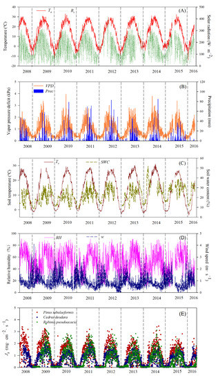
Figure 1.
Temporal dynamics of the daily mean air temperatures (Ta), daily mean total solar radiation (Rs) (A), daily mean vapor pressure deficit (VPD), daily precipitation (Prec) (B), daily mean soil temperature at 10 cm (Ts), daily mean soil water content at 10 cm (SWC) (C), daily mean relative humidity (RH), daily mean wind speed (w) (D), and daily mean sap flux density of three trees (E) in Beijing Teaching Botanical Garden, China during 2008 and 2016.
2.4. Data Analysis
An analysis of variance (ANOVA) was used to explore the effects of tree species and years on sap flux density. Post-hoc least significant difference tests were performed only when significant differences were detected by ANOVA. The results were regarded as statistically significant or extremely significant when the p value was less than the significance level of 0.05 or 0.01, respectively.
Pearson correlation analysis was implemented to explore the significance of the relationship of the sap flux density for three tree species with environmental influencing factors in different timescales (p < 0.05 or p < 0.01). At a daily scale, the model of sap flux density was developed based on the Jarvis–Stewart equation, due to the nonlinear relationships between the sap flux density and the main influencing factors.
Jarvis [36] proposed a serial empirical formula to express the relationship between leaf stomatal conductance and environmental factors; this formula has been widely used and modified [37,38]. Transpiration and sap flow have also been linked directly with environmental factors by analogy with the stomatal conductance formulation [39,40,41,42]. In this study, we used sap flux density to investigate the environmental controls using Equation (3).
Equations (4)–(6) are stress functions of Ta, Rs, and VPD [36,37,39]. Jmax is the observed maximum value for each tree species during the study periods. Tp is the optimal temperature for maximum sap flux density. k1 and k2 are the rate of change between Js and Ta, Rs, respectively. Rm is the maximum radiation during the study periods. k3 and k4 are the rate of change between Js and VPD at lower and higher atmospheric demand, respectively [39]. Model performances were examined using the coefficient of determination (R2) and the root mean square error (RMSE) between observations and simulations [41].
At seasonal and interannual scales, the models in sap flux density were developed by the multivariate regression equation.
All statistical analyses were performed with SPSS 16.0 software (SPSS for Windows, version 16.0, Chicago, IL, USA). Figures were plotted using Sigmaplot 10.0 software (Sigmaplot for windows, version 10.0, San Jose, CA, USA).
3. Results
3.1. Environmental Variations
Daily variations in major environmental parameters are summarized in Figure 1A–D over 2008–2016. Daily mean Ta and Ts increased from winter to summer ranging from −15.04 °C to 33.11 °C and −3.75 °C to 31.05 °C in each year, respectively. The monthly mean Ta (Ts) varied between −2.47 °C (−0.93 °C) in January and 27.42 °C (26.80 °C) in July. Annual means of Ts varied from year to year, with means of 11.0–14.4 °C. Daily mean Rs had its highest value (419.91 W·m−2) in summer and its lowest value (1.81 W·m−2) in winter (Figure 1A). Monthly Rs was highest in May and lowest in December, with values of 227.57 W·m−2 and 80.87 W·m−2, respectively. Annual mean Rs varied from 136.76 W·m−2 (2009) to 166.25 W·m−2 (2013).
The variation of daily mean VPD was similar with Ta and Rs, with the highest value in summer and lowest value in winter (Figure 1B). Daily mean VPD peaked at 3.96 kPa in July in 2010. Monthly mean VPD varied between 0.35 kPa (in January) and 1.63 kPa (in May). Annual mean VPD varied from 0.86 kPa (2008) to 1.06 kPa (2014). Daily mean RH was higher in summer and lower in spring and winter. The range of daily mean RH was 8.65%–91.14% across eight years (Figure 1D). Annual mean RH was highest in 2008, 51.7%, and lowest in 2014, 46.2%. The maximum of daily mean w occurred mostly in spring (Figure 1D). Annual mean w varied from 0.76 m·s−1 (2015) to 1.05 m·s−1 (2008). Interannual monthly mean Ta, Ts, RH, and Prec were highest in July and VPD was highest in May.
The daily precipitation was concentrated from May to September (>80% of the total) and the lowest value occurred in winter (Figure 1B). Precipitation totaled 4704 mm over the eight years, with the maximum value occurring in 2011 (755.8 mm), which was 61.7% greater than the minimum value (467.5 mm) in 2015. Interannual monthly mean Prec was the highest in July and the lowest in December over eight years, with a value of 1335.9 mm and 12.4 mm, respectively. SWC varied significantly during the year due to urban irrigation but was not regulated by individual rainfall events. The highest values of SWC were in summer and the lowest in winter (Figure 1C). During the period of observation, annual mean SWC was the highest in 2015 (26.95%) and the lowest in 2008 (17.07%).
The pattern of day-to-day variation and the interannual monthly mean variation in the Js of three urban tree species corresponded closely to environmental conditions, such as changes in Ta, Ts, Rs, and VPD (Figure 1).
3.2. Variations in the Sap Flux Density of Different Urban Trees
3.2.1. Daily Variation
The patterns of day-to-day variation in the Js of three urban tree species were shown in Figure 1E. In 2008–2015, the daily mean Js of Pinus tabulaeformis, Cedrus deodara, and Robinia pseudoacacia ranged from 0.0001 to 3.45 mg·cm−2·s−1, 0.0002 to 2.11 mg·cm−2·s−1, and 0.003 to 3.64 mg·cm−2·s−1, respectively. The daily mean Js of three urban tree species gradually increased in spring, peaking in summer with values varying from 2.63 to 3.45 mg·cm−2·s−1, 1.49 to 2.11 mg·cm−2·s−1, and 2.38 to 3.64 mg·cm−2·s−1 and then decreased in winter, over the eight years.
The sap flux density of coniferous species (Pinus tabulaeformis and Cedrus deodara) started up earlier in spring than that of the deciduous specie (Robinia pseudoacacia). The maximum daily mean Js of Pinus tabulaeformis, Cedrus deodara, and Robinia pseudoacacia was 3.38, 3.21, 2.70, 3.04, 3.18, 2.63, 3.45, 2.80 mg·cm−2·s−1, 1.84, 2.11, 1.49, 1.72, 1.74, 1.69, 1.81, 1.61 mg·cm−2·s−1, and /, 3.64, 2.81, 2.80, 2.78, 2.82, 3.11, 2.38 mg·cm−2·s−1 in years from 2008 to 2015, respectively. The maximum of the sap flux density of Pinus tabulaeformis was highest, followed by Robinia pseudoacacia and Cedrus deodara.
The mean diurnal variations of sap flux density of the three tree species were observed on a typical sunny day in each season over eight years (Figure 2). The hourly sap flux density of Pinus tabulaeformis was higher than that of Cedrus deodara in four seasons. The maximum of the hourly sap flux density of Pinus tabulaeformis and Cedrus deodara were at 12:00–13:00 p.m.; the maximum differences were 1.18 mg·cm−2·s−1 and 1.64 mg·cm−2·s−1 in spring and summer, respectively. The maximum of the hourly sap flux density of Pinus tabulaeformis and Cedrus deodara were at 15:00 p.m. and 13:00 p.m. in autumn, respectively, and the maximum difference was 0.66 mg·cm−2·s−1. In winter, the maximum of the hourly sap flux density of Pinus tabulaeformis and Cedrus deodara were at 7:00 a.m., and the maximum difference was 0.12 mg·cm−2·s−1.
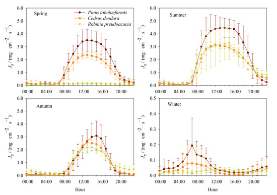
Figure 2.
Comparison of the diurnal patterns of the interannual mean sap flux density among three urban trees species (Pinus tabulaeformis Carrière, Cedrus deodara (Roxb.) G. Don, and Robinia pseudoacacia Linn.) for four seasons in 2008–2015. Dates are expressed as mean ± SD.
The hourly sap flux density of Robinia pseudoacacia was almost zero in spring and winter, which was lower than that of Pinus tabulaeformis and Cedrus deodara. In summer, the hourly sap flux density of Robinia pseudoacacia was consistent with that of Cedrus deodara but lower than that of Pinus tabulaeformis with the maximum difference of 1.31 mg·cm−2·s−1. The sap flux density Robinia pseudoacacia at night was higher than that of Pinus tabulaeformis and Cedrus deodara, and the sap flow started up earlier than them in summer and autumn.
3.2.2. Seasonal Variation
The start-up time of the sap flow of Pinus tabulaeformis and Cedrus deodara (March) was earlier than that of Robinia pseudoacacia (May) in spring and reached the peak at the same time. The interannual monthly mean of the Js of Pinus tabulaeformis, Cedrus deodara, and Robinia pseudoacacia was highest in August with values of 1.91, 1.18, and 1.54 mg·cm−2·s−1, respectively (Figure 3A). The mean Js of Pinus tabulaeformis was higher than that of Cedrus deodara and Robinia pseudoacacia in each month. The mean Js of Robinia pseudoacacia was higher than that of Cedrus deodara from June to October.
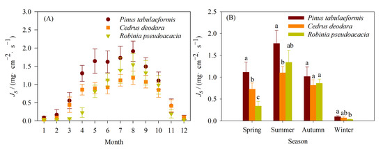
Figure 3.
Comparison of the monthly mean values (A) and seasonal mean values (B) of the sap flux density among the three urban tree species (Pinus tabulaeformis, Cedrus deodara, and Robinia pseudoacacia) in 2008 to 2015. (Dates are expressed as mean ± SD. Different small letters denote significant differences among three tree species at the significant level of 0.05).
The seasonal mean sap flux density of the three tree species was the highest in summer and the lowest in winter (Figure 3B). The seasonal mean Js of Pinus tabulaeformis, Cedrus deodara, and Robinia pseudoacacia in summer were 18.67, 16.19, and 41.62 times that in winter in 2008–2015.
The variations among the three tree species were different in four seasons. In spring, there were significant differences in the mean sap flux density among three trees species (p < 0.05). The mean sap flux density of Pinus tabulaeformis was 53.16% and 228.40% higher than that of Cedrus deodara and Robinia pseudoacacia, respectively. In summer, the mean sap flux density of Pinus tabulaeformis, followed by Robinia pseudoacacia and Cedrus deodara. The mean sap flux density of Pinus tabulaeformis (1.77 mg·cm−2·s−1) was significantly higher than that of Cedrus deodara (1.10 mg·cm−2·s−1) (p < 0.05). There were no significant differences between the mean sap flux density of Robinia pseudoacacia and both Pinus tabulaeformis and Cedrus deodara (p > 0.05). There were no significant differences in the mean sap flux density among the three tree species in autumn (p > 0.05). In winter, the mean sap flux density of Pinus tabulaeformis was highest and that of Robinia pseudoacacia was lowest. The mean sap flux density of Pinus tabulaeformis was 2.95 times that of Robinia pseudoacacia (p < 0.05).
3.2.3. Interannual Variation
The interannual variation in the Js of the three urban tree species was shown in Figure 4. There were no significant effects from the years on the Js of the three tree species, but tree species had significant effects on Js. The annual mean sap flux density of Pinus tabulaeformis was the highest (0.995 mg·cm−2·s−1), followed by Robinia pseudoacacia (0.684 mg·cm−2·s−1) and Cedrus deodara (0.679 mg·cm−2·s−1) over eight years. The annual mean sap flux density of Pinus tabulaeformis was significantly higher than that of Cedrus deodara and Robinia pseudoacacia in 2008, 2012, and 2014 (p < 0.05). There were no significant differences between the mean sap flux density of Cedrus deodara and Robinia pseudoacacia except in 2015 (p > 0.05). The annual mean sap flux density of Pinus tabulaeformis was 1.62, 1.52, 1.44, 1.29, 1.44, 1.45, 1.72, 1.25 (1.45, 1.40, 1.28, 1.26, 1.49, 1.35, 1.82, 1.81) times that of Cedrus deodara (Robinia pseudoacacia) in 2008–2015.
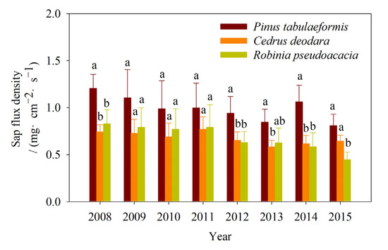
Figure 4.
Comparison of the annual mean values of the sap flux density among the three urban tree species (Pinus tabulaeformis, Cedrus deodara, and Robinia pseudoacacia) in 2008 to 2015. (Dates are expressed as mean ± SD. Different small letters denote significant differences among the three tree species at a significance level of 0.05).
3.3. Response of the Sap Flux Density to Environmental Variables
The responses of the sap flux density for three urban tree species to environmental factors in different time scales were shown in Table 2. The results showed that the correlations between the sap flux density of the three tree species and environmental factors were different in different time scales.
Table 2.
Correlation between the sap flux density of the three urban tree species and the environmental factors at different time scales.
3.3.1. Daily Scale
In a daily scale, the sap flux density of the three tree species was significantly positively correlated with Ta, Rs, VPD, Ts, SWC, and RH and negatively correlated with w (p < 0.01). The correlation coefficients were larger between sap flux density and Ta, Ts, VPD, and Rs and lower between sap flux density and SWC, RH, and w.
The Jarvis–Stewart model was used to construct the equation between sap flux density and environmental factors due to their nonlinear relationships. The Jarvis–Stewart model based on three main environmental variables (Ta, Rs, and VPD) can simulate Js well for the three tree species (Figure 5). The model parameters were fitted with the diurnal sap flow data to form the parameterized Js model of the three tree species (Table 3).
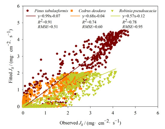
Figure 5.
Comparison between the estimated and observed sap flux density of three tree species.
Table 3.
Parameters from the optimization of the modified Jarvis–Stewart model estimating the sap flux density for the three tree species.
The fitting results showed that the Js model kept high simulation accuracy for Pinus tabulaeformis (R2 = 0.91, p < 0.01), Cedrus deodara (R2 = 0.74, p < 0.01), and Robinia pseudoacacia (R2 = 0.78, p < 0.01). This indicates that the modeling is producing a reasonable description of the observed data. RMSE can reflect the deviation between the fitted and the observed values of the model. The smaller the value of RMSE, the better the effect of simulation. The simulation effect of the model was the highest for Pinus tabulaeformis (RMSE = 0.51), followed by Cedrus deodara (RMSE = 0.60) and Robinia pseudoacacia (RMSE = 0.95).
3.3.2. Seasonal Scale
In a seasonal scale, the sap flux density of the three tree species was also significantly positively correlated with Ta, Rs, VPD, Prec, Ts, SWC, and RH and negatively correlated with w (p < 0.01) (Table 2).
Stepwise regression analysis was adopted to analyze the influence of environmental factors on the sap flux density of the three tree species in a seasonal scale and obtain the relevant equations (Table 4). In a seasonal scale, 89.2% of the variation in the Js of Pinus tabulaeformis was explained by mean Ta and SWC, 84.9% of the variation in Cedrus deodara by Ta, and 90.1% of the variation in Robinia pseudoacacia by Ts, SWC, and w (Table 4; p < 0.05).
Table 4.
Multivariate regression equation of the mean sap flux density and the selected main environmental variables in seasonal and interannual scales in 2008–2015 in Beijing Teaching Botanical Garden. The determination of the variables was shown, and the insignificant parameters were automatically eliminated from the regressions model.
3.3.3. Interannual Scale
The correlations between the sap flux density and the environmental factors in an interannual scale were also analyzed (Table 2). The results showed that the annual average sap flux density of Pinus tabulaeformis and Robinia pseudoacacia was significant positive correlated with w and negatively correlated with SWC (p < 0.05). There was no significant correlation between the annual average sap flux density of Cedrus deodara and environmental factors (p > 0.05).
Similarly, stepwise regression analysis was used to analyze the relationship between the sap flux density of the three tree species and environmental factors in an interannual scale (Table 4). The results showed that 68.2% of the variation in the Js of Pinus tabulaeformis was explained by mean w and 64.9% of the variation in Robinia pseudoacacia by SWC. However, there were no environmental factors selected that were entered into the regression equation of the mean sap flux density of Cedrus deodara. The result indicated that the selected environmental factors could not explain the variation in the sap flux density of Cedrus deodara, and the main factors affecting it need to be further studied in interannual scale.
4. Discussion
4.1. Variations in the Sap Flux Density of the Three Urban Tree Species
The physiological structure of trees determines their potential for transpiration [9,43]. The difference in physiological structure among tree species will lead to a difference in canopy and boundary layer conductance and then affect the transpiration of trees [5]. The characteristics of tree species such as age, height, DBH, sapwood allocation, canopy structure, leaf phenology, and leaf area index also resulted in a difference in sap flow among tree species [44,45,46,47]. At the same time, the stomata of tree leaves regulate sap flow in response to environmental changes to ensure their optimal growth [48]. The response mechanism of different tree species to environmental factors was different [49]. Therefore, different tree species with diverging traits regarding environmental variables lead to species-specific differences in transpiration.
In this study, we found that there were significant differences on sap flux density among the three tree species (Figure 1, Figure 2, Figure 3 and Figure 4). The results were similar with Liu et al. [50] and Pataki et al. [45]. The transpiration strategies of different tree species in the same area were different [51,52]. Usually plant sap flow occurs during the day and stops at night due to the closure of stomata in plant leaves. However, in this study, the diurnal dynamics of the three species showed that there was weak sap flow at night, especially in Robinia pseudoacacia. Similar phenomena have been found in many tree species in other regions [29,53]. The possible reason was that the sap flow of the tree was too strong during the day, and the tree loses too much water, leading to the imbalance of water supply and consumption. The root system absorbs water at night to replenish the water deficit during the day [8]. In addition, the stomata of some tree species are kept open at night, driven by environmental factors, to increase sap flow [29].
The start and end times of daily sap flow were different among the three tree species, which may be due to the different water storage capacity of the different tree species. The mean sap flux density of Pinus tabulaeformis was higher than the other tree species. This result was inconsistent with many studies showing that the sap flux density of broadleaved species was higher than that of conifer species [54]. The water transport capacity of the ducts of deciduous trees was stronger than that of the tracheids of conifer trees [55]. At the same time, the leaf cuticle of conifers was thick, and the stomatal conductance was significantly lower than that of deciduous trees [55,56]. This study was located in an urban environment, where trees were susceptible to heat and drought, leading to trunk embolism. Some studies have shown that the embolization vulnerability of ring pore wood species was greater than that of conifers [57], which may be the reason for the lower sap flux density of Robinia pseudoacacia (ring pore wood species) than that of Pinus tabulaeformis.
Evergreen species (Pinus tabulaeformis and Cedrus deodara) had higher sap flux density than deciduous species (Robinia pseudoacacia) in spring and winter [14,58]. However, the annual mean sap flux density of Pinus tabulaeformis was highest and Cedrus deodara was lowest. The main reason is that different tree species had different response and sensitivity to environmental factors, such as stomatal opening [52]. Further, the study indicated that the sap flux density of the three tree species was less during non-growing seasons (November to April) than growing seasons (May to October), which could be partly caused by leaf senescence and shedding in the non-growing season [59]. The annual mean Js in the growing season was 2.65–6.24 times that in the non-growing season in 2008–2015. This study indicated the significant seasonal variation in Js, which is consistent with many previous studies [46,59].
Previous studies had reported low interannual variability in the sap flow of upland forests [60,61]. However, Zhao et al. [46] monitored the annual variation of sap flow in mature Acacia mangium for four years, and the results showed that the total water consumption of transpiration varied significantly between years. Han et al. [62] measured the sap flow of a Pinus sylvestris var. mongolica stand on the southern margin of Horqin sandy land, and the results also showed that there were significant interannual differences in the sap flow of Pinus sylvestris var. Mongolica. The variation of sap flow was consistent with the interannual variation trend of hydrological environment characteristics [63]. In this study, annual Js remained relatively stable over the observation period. The cause may be the adequate soil water in our study site, which was irrigated often in urban areas.
4.2. Environmental Control of the Sap Flux Density of the Three Tree Species in Different Time Scales
In addition to its physiological structure, tree sap flow is also affected by meteorological factors, such as atmospheric temperature, solar radiation, air relative humidity, wind speed, precipitation, and soil factors, such as soil temperature and humidity [64]. The variations in climate lead to substantial seasonal variation in the environmental variables and then tree sap flow variations. Meteorological factors determine the instantaneous change of sap flux density, and soil factors determine the overall level of the sap flow [4,5]. These environmental factors influence the sap flow of trees in various ways [49].
Air temperature and air relative humidity directly affect the sap flow of trees. Solar radiation can determine the change in air temperature and relative humidity and induce the opening and closing of leaf stomata [65]. Vapor pressure deficit (VPD) can be calculated by air temperature and relative humidity, so it can better reflect the change in the transpiration water consumption of trees [66]. Wind speed indirectly affects plant sap flow, mainly by changing leaf temperature, air temperature, and air relative humidity [67]. Soil water content is the main limiting factor of plant growth, which directly affects the absorption of soil nutrients by plant roots [68]. Precipitation is the main natural source to recover soil water, which provides available water for plant sap flow [69,70]. A large number of studies had shown that plant sap flow shows a certain difference in response to environmental factors [29,31,64]. The dominant factors affecting sap flow were different in different regions, tree species, and time scales, which is related to plant response mechanisms to environmental conditions. However, solar radiation and water vapor pressure deficit have always been regarded as the most important meteorological factors affecting sap flow [71,72].
In a daily scale, there were more environmental factors affecting the sap flux density of the three tree species. The main factors affecting the sap flux density of the three tree species were Ta, Rs, VPD, and Ts. The results were consistent with previous studies [32]. The sap flow of urban trees is strongly coupled with atmospheric demand and photosynthetic activity. The results of the Jarvis–Stewart model simulation showed that the sap flux density of different urban tree species had different responses to environmental factors (Ta, Rs, and VPD). The model is more suitable for the sap flux density simulation of Pinus tabulaeformis than Cedrus deodara and Robinia pseudoacacia in this study. The simulation effect of the model was also related to the tree species. This result was consistent with previous studies [41].
In a seasonal scale, the explanatory quantities (84.9%–90.1%) of the variation in sap flux density explained by environmental factors were higher than that in an interannual scale (64.9%–68.2%). The main factors affecting the sap flux density of Pinus tabulaeformis (Cedrus deodara and Robinia pseudoacacia) were Ta and SWC (Ta and Ts, SWC, w). The results indicated that the sap flux density of Robinia pseudoacacia was more affected by soil factors. The increase of soil temperature was beneficial for the root to absorb water and promote sap flow. At the same time, soil temperature affected tree sap flow by controlling soil water content [73]. This study demonstrated the importance of soil temperature on the sap flux density of trees, which should be strengthened in future studies on tree sap flow.
The interannual variations in the Js of Pinus tabulaeformis and Robinia pseudoacacia were mainly influenced by w and SWC, respectively. However, the selected environmental factors could not explain the variation in the sap flux density of Cedrus deodara, and the main factors affecting it need to be further studied. The effect of w on plant sap flow is relatively complex. Wind can take away the humid air around the leaves of trees and accelerate the diffusion of water vapor, thus increasing the sap flow of plants. However, when the wind speed is too high, the leaves lose water rapidly, the plants develop their defense mechanism (stomatal closure of the leaves), and the surface temperature of the leaves decreases, which leads to a reduction in the sap flux density of trees [67]. The mechanism of the influence of wind speed on the sap flux density of trees needed further study. Soil water content was a major determinant of the interannual variation in tree sap flow [74,75]. Yoshifuji et al. [76] found that the interannual variation in the sap flow of a mature plantation in Thailand was positively linked with soil water. The interannual sap flow change was positively correlated with soil water content for a Robinia pseudoacacia plantation on the Loess Plateau [10]. The effect of soil water content on sap flux density was also complex, and the response of sap flux density to soil water content was different with different time, weather and soil depth.
Interannually, the influence of environmental variables on Js has seldom been documented for urban areas. Previous studies have shown that, unlike Ta, Rs, and VPD, which influence sap flow at short time scales, wind speed and soil water availability would be important drivers of sap flow at longer time scales [77]. Our findings were consistent with their conclusions. At long time scales, suitable w and SWC were key factors controlling Js, since moderate wind and water availability were essential for promoting plant growth.
5. Conclusions
We investigated the difference in the sap flux density of Pinus tabulaeformis, Cedrus deodara, and Robinia pseudoacacia and their main environmental influencing factors in different time scales in the urban settings of Beijing. There were significant differences in the sap flux density of the three tree species in daily, seasonal, and interannual timescales in this study. The start-up time of the monthly sap flow of Pinus tabulaeformis and Cedrus deodara (March) was earlier than that of Robinia pseudoacacia (May) in spring and reached the peak in August. The hourly, seasonal, and annual mean sap flux densities of Pinus tabulaeformis were higher than that of Cedrus deodara and Robinia pseudoacacia. The hourly and seasonal mean sap flux density of Robinia pseudoacacia was higher than that of Cedrus deodara in summer. The annual mean sap flux density of Pinus tabulaeformis was 1.25–1.72 and 1.26–1.82 times that Cedrus deodara and Robinia pseudoacacia in 2008–2015. There were no significant differences between the annual mean sap flux density of Cedrus deodara and Robinia pseudoacacia except in 2015. The sap flux density of deciduous species (Robinia pseudoacacia) was lower than that of conifer species (Pinus tabulaeformis). There were no significant effects of years on the Js of the three tree species.
The Js responses of the three tree species to environmental factors varied differently from daily to interannual timescales. The pattern of the day-to-day variation in the Js of the three urban tree species corresponded closely to Ta, Ts, Rs, and VPD. The Jarvis–Stewart model based on three environmental variables (Ta, Rs, and VPD) can simulate Js well for three tree species. The model is more suitable for the sap flux density simulation of Pinus tabulaeformis than of Cedrus deodara and Robinia pseudoacacia. Regression analysis results showed that the main factor affecting the sap flux density of Pinus tabulaeformis and Cedrus deodara was Ta in a seasonal timescale. However, the main factor affecting the sap flux density of Robinia pseudoacacia was Ts. The interannual variations in the Js of Pinus tabulaeformis and Robinia pseudoacacia were mainly influenced by w and SWC, respectively. The selected environmental factors could not explain the variation in the sap flux density of Cedrus deodara, and the main factors affecting it need to be further studied.
Author Contributions
Conceptualization, Y.C. and X.W.; data curation, H.Z. and X.S.; formal analysis, Y.C.; funding acquisition, Y.C. and X.W.; methodology, Y.C. and X.W.; supervision, X.W.; validation, X.W.; writing—original draft, Y.C.; writing—review and editing, Y.C. and X.W. All authors have read and agreed to the published version of the manuscript.
Funding
This research was supported by the National Nature Science Foundation of China (32101318).
Data Availability Statement
The data presented in this study are available from corresponding author upon reasonable request.
Conflicts of Interest
The authors declare no conflict of interest.
References
- Nowak, D.J.; Dwyer, J.F. Understanding the benefits and costs of urban forest ecosystems. In Urban and Community Forestry in the Northeast; Springer: Dordrecht, The Netherlands, 2007; pp. 25–46. [Google Scholar]
- Andréassian, V. Waters and forests: From historical controversy to scientific debate. J. Hydrol. 2004, 291, 1–27. [Google Scholar] [CrossRef]
- Aparecido, L.M.T.; Miller, G.R.; Cahill, A.T.; Moore, G. Comparison of tree transpiration under wet and dry canopy conditions in a Costa Rican premontane tropical forest. Hydrol. Process. 2016, 30, 5000–5011. [Google Scholar] [CrossRef]
- Jiao, L.; Lu, N.; Fang, W.W.; Li, Z.S.; Wang, J.; Jin, Z. Determining the independent impact of soil water on forest: A case study of a black locust plantation in the Loess Plateau, China. J. Hydrol. 2019, 572, 671–681. [Google Scholar] [CrossRef]
- Wullschleger, S.D.; Meinzer, F.C.; Vertessy, R.A. A review of whole-plant water use studies in trees. Tree Physiol. 1998, 18, 499–512. [Google Scholar] [CrossRef] [PubMed]
- Burgess, S.S.O. Measuring transpiration responses to summer precipitation in a Mediterranean climate: A simple screening tool for identifying plant water-use strategies. Physiol. Plantarum 2006, 127, 404–412. [Google Scholar] [CrossRef]
- Dammeyer, H.C.; Schwinning, S.; Schwartz, B.F.; Moore, G.W. Effects of juniper removal and rainfall variation on tree transpiration in a semi-arid karst: Evidence of complex water storage dynamics. Hydrol. Process. 2016, 30, 4568–4581. [Google Scholar] [CrossRef]
- Granier, A.; Huc, R.; Barigah, S.T. Transpiration of natural rain forest and its dependence on climatic factors. Agric. Forest Meteorol. 1996, 78, 16–29. [Google Scholar] [CrossRef]
- Huang, Y.Q.; Zhao, P.; Zhang, Z.F.; Li, X.K.; He, C.X.; Zhang, R.Q. Transpiration of Cyclobalanopsis glauca (syn. Quercus glauca) stand measured by sap-flow method in a karst rocky terrain during dry season. Ecol. Res. 2009, 24, 791–801. [Google Scholar]
- Zhang, J.G.; Guan, J.H.; Shi, W.Y.; Yamanaka, N.; Du, S. Interannual variation in stand transpiration estimated by sap flow measurement in a semi-arid black locust plantation, Loess Plateau, China. Ecohydrology 2015, 8, 137–147. [Google Scholar] [CrossRef]
- Banin, L.; Lewis, S.L.; Lopez-Gonzalez, G.; Baker, T.R.; Quesada, C.A.; Chao, K.J.; Burslem, D.F.R.P.; Nilus, R.; Salim, K.A.; Keeling, H.C.; et al. Tropical forest wood production: A cross-continental comparison. J. Ecol. 2014, 102, 1025–1037. [Google Scholar] [CrossRef]
- Siddiq, Z.; Chen, Y.J.; Zhang, Y.J.; Zhang, J.L.; Cao, K.F. More sensitive response of crown conductance to VPD and larger water consumption in tropical evergreen than in deciduous broadleaf timber trees. Agric. Forest Meteorol. 2017, 247, 399–407. [Google Scholar] [CrossRef]
- Ma, L.; Lu, P.; Zhao, P.; Rao, X.Q.; Cai, X.A.; Zeng, X.P. Diurnal, daily, seasonal and annual patterns of sap-flux-scaled transpiration from an Acacia mangium plantation in South China. Ann. Forest Sci. 2008, 65, 402. [Google Scholar] [CrossRef]
- Siddiq, Z.; Cao, K.F. Increased water use in dry season in eight deiperocarp species in a common plantation in the northern boundary of Asian tropics. Ecohydrology 2016, 9, 871–881. [Google Scholar] [CrossRef]
- Fischer, R.; Armstrong, A.; Shugart, H.H.; Huth, A. Simulating the impacts of reduced rainfall on carbon stocks and net ecosystem exchange in a tropical forest. Environ. Modell. Softw. 2014, 52, 200–206. [Google Scholar] [CrossRef]
- Lens, F.; Sperry, J.S.; Christman, M.A.; Choat, B.; Rabaey, D.; Jansen, S. Testing hypotheses that link wood anatomy to cavitation resistance and hydraulic conductivity in the genus Acer. New Phytol. 2011, 190, 709–723. [Google Scholar] [CrossRef]
- Llorens, P.; Poyatos, R.; Latron, J.; Delgado, J.; Oliveras, I.; Gallart, F. A multi-year study of rainfall and soil water controls on Scots pine transpiration under Mediterranean mountain conditions. Hydrol. Process. 2010, 24, 3053–3064. [Google Scholar] [CrossRef]
- Tan, Z.H.; Cao, M.; Yu, G.R.; Tang, J.W.; Deng, X.B.; Song, Q.H.; Tang, Y.; Zheng, Z.; Liu, W.J.; Feng, Z.L.; et al. High sensitivity of a tropical rainforest to water variability: Evidence from 10 years of inventory and eddy flux data. J. Geophys. Res. 2013, 118, 9393–9400. [Google Scholar] [CrossRef]
- Litvak, E.; McCarthy, H.R.; Pataki, D.E. A method for estimating transpiration of irrigated urban trees in California. Landscape Urban Plan. 2017, 158, 48–61. [Google Scholar] [CrossRef]
- Mini, C.; Hogue, T.S.; Pincetl, S. Estimation of residential outdoor water use in Los Angeles, California. Landscape Urban Plan. 2014, 127, 124–135. [Google Scholar] [CrossRef]
- Berthier, E.; Dupont, S.; Mestayer, P.G.; Andrieu, H. Comparison of two evapotranspiration schemes on a suburban site. J. Hydrol. 2006, 328, 635–646. [Google Scholar] [CrossRef]
- Mitchell, V.G.; Cleugh, H.A.; Grimmond, C.S.B.; Xu, J. Linking urban water balance and energy balance models to analyse urban design options. Hydrol. Process. 2008, 22, 2891–2900. [Google Scholar] [CrossRef]
- Christen, A.; Vogt, R. Energy and radiation balance of a central European city. Int. J. Climatol. 2004, 24, 1395–1421. [Google Scholar] [CrossRef]
- Simon, H.; Lindén, J.; Hoffmann, D.; Braun, P.; Bruse, M.; Esper, J. Modeling transpiration and leaf temperature of urban trees-A case study evaluating the microclimate model ENVI-met against measurement data. Landscape Urban Plan. 2018, 174, 33–40. [Google Scholar] [CrossRef]
- Law, B.E.; Falge, E.; Gu, L.; Baldocchi, D.D.; Bakwin, P.; Berbigier, P.; Davis, K.; Dolman, A.J.; Falk, M.; Fuentes, J.D.; et al. Environmental controls over carbon dioxide and water vapor exchange of terrestrial vegetation. Agric. Forest Meteorol. 2002, 113, 97–120. [Google Scholar] [CrossRef]
- Hagishima, A.; Narita, K.; Tanimoto, J. Field experiment on transpiration from isolated urban plants. Hydrol. Process. 2007, 21, 1217–1222. [Google Scholar] [CrossRef]
- McLaughlin, S.B.; Wullschleger, S.D.; Sun, G.; Nosal, M. Interactive effects of ozone and climate on water use, soil moisture content and streamflow in a southern Appalachian forest in the USA. New Phytol. 2007, 174, 125–136. [Google Scholar] [CrossRef]
- Granier, A. Evaluation of transpiration in a Douglas-fir stand by means of sap flow measurements. Tree Physiol. 1987, 3, 309–320. [Google Scholar] [CrossRef]
- Fang, W.W.; Lü, N.; Fu, B.J. Research advances in nighttime sap flow density, its physiological implications, and influencing factors in plants. Acta Ecol. Sin. 2018, 38, 7521–7529. (In Chinese) [Google Scholar]
- Wang, K.Y.; Kellomäki, S.; Zha, T.; Peltola, H. Annual and seasonal variation of sap flow and conductance of pine trees grown in elevated carbon dioxide and temperature. J. Exp. Bot. 2005, 56, 155–165. [Google Scholar] [CrossRef][Green Version]
- Wang, Y.N.; Cao, G.X.; Wang, Y.H.; Webb, A.A.; Yu, P.T.; Wang, X.J. Response of the daily transpiration of a larch plantation to variation in potential evaporation, leaf area index and soil moisture. Sci. Rep. 2019, 9, 4697. [Google Scholar] [CrossRef]
- Wang, H.; Ouyang, Z.Y.; Chen, W.P.; Wang, X.K.; Zheng, H.; Ren, Y.F. Water, heat, and airborne pollutants effects on transpiration of urban trees. Environ. Pollut. 2011, 159, 2127–2137. [Google Scholar] [CrossRef] [PubMed]
- Zhao, P.; Rao, X.Q.; Ma, L.; Cai, X.A.; Zeng, X.P. Application of Granier’s sap flow system in water use of Acacia mangium forest. J. Trop. Subtrop. Bot. 2005, 13, 457–468. (In Chinese) [Google Scholar]
- Falge, E.; Baldocchi, D.; Olsam, R.J.; Anthoni, P.; Aubinet, M.; Bernhofer, C.; Burba, G.; Ceulemans, R.; Clement, R.; Dolman, H.; et al. Gap filling strategies for defensible annual sums of net ecosystem exchange. Agric. Forest Meteorol. 2001, 107, 43–69. [Google Scholar] [CrossRef]
- Campbell, G.S.; Norman, J.M. An Introduction to Environmental Biophysics; Springer: New York, NY, USA, 1998. [Google Scholar]
- Jarvis, P.G. The interpretation of the variations in leaf water potential and stomatal conductance found in canopies in the field. Philos. Trans. R. Soc. Lond. 1976, 273, 593–610. [Google Scholar]
- Stewart, J.B. Modelling surface conductance of pine forest. Agric. For. Meteorol. 1988, 43, 19–35. [Google Scholar] [CrossRef]
- Whitley, R.; Medlyn, B.; Zeppel, M.; Macinnis-Ng, C.; Eamus, D. Comparing the Penman-Monteith equation and a modified Jarvis-Stewart model with an artificial neural network to estimate stand-scale transpiration and canopy conductance. J. Hydrol. 2009, 373, 256–266. [Google Scholar] [CrossRef]
- Whitley, R.; Zeppel, M.; Armstrong, N.; Macinnis-Ng, C.; Yunusa, I.; Eamus, D. A modified Jarvis-Stewart model for predicting stand-scale transpiration of an Australian native forest. Plant Soil 2008, 305, 35–47. [Google Scholar] [CrossRef]
- Whitley, R.; Taylor, D.; Macinnis-Ng, C.; Zeppel, M.; Yunusa, I.; O’Grady, A.; Froend, R.; Medlyn, B.; Eamus, D. Developing an empirical model of canopy water flux describing the common response of transpiration to solar radiation and VPD across five contrasting woodlands and forests. Hydrol. Process. 2013, 27, 1133–1146. [Google Scholar] [CrossRef]
- Wang, H.L.; Guan, H.D.; Liu, N.; Soulsby, C.; Tetzlaff, D.; Zhang, X.P. Improving the Jarvis-type model with modified temperature and radiation functions for sap flow simulations. J. Hydrol. 2020, 587, 124981. [Google Scholar] [CrossRef]
- Yu, S.P.; Guo, J.B.; Liu, Z.B.; Wang, Y.H.; Ma, J.; Li, J.M.; Liu, F. Assessing the impact of soil moisture on canopy transpiration using a modified Jarvis-Stewart model. Water 2021, 13, 2720. [Google Scholar] [CrossRef]
- Chen, L.X.; Li, Z.D.; Zhang, Z.Q.; Zhang, W.J.; Zhang, X.F.; Dong, K.Y.; Wang, G.Y. Environmental responses of four urban tree species transpiration in northern China. Chin. J. Appl. Ecol. 2009, 20, 2861–2870. (In Chinese) [Google Scholar]
- McJannet, D.; Fitch, P.; Disher, M.; Wallace, J. Measurements of transpiration in four tropical rainforest types of north Queensland, Australia. Hydrol. Process. 2007, 21, 3549–3564. [Google Scholar] [CrossRef]
- Pataki, D.E.; McCarthy, H.R.; Litvak, E.; Pincetl, S. Transpiration of urban forests in the Los Angeles metropolitan area. Ecol. Appl. 2011, 21, 661–677. [Google Scholar] [CrossRef]
- Zhao, P.; Zou, L.L.; Rao, X.Q.; Ma, L.; Ni, G.Y.; Zeng, X.P.; Cai, X. Water consumption and annual variation of transpiration in mature Acacia mangium Plantation. Acta Ecol. Sin. 2011, 31, 6038–6048. (In Chinese) [Google Scholar]
- Zhang, J. Effects of Environmental Factors on Sap Flow and Radial Growth of Poplar Plantation. Master’s Thesis, Beijing Forestry University, Beijing, China, 2019. (In Chinese). [Google Scholar]
- Chen, L.X. Environmental Response and Biophysical Control over Transpiration by Trees/Stands. Ph.D. Thesis, Beijing Forestry University, Beijing, China, 2013. (In Chinese). [Google Scholar]
- Huang, J.; Kong, F.H.; Yin, H.W.; Middel, A.; Liu, H.Q.; Zheng, X.D.; Wen, Z.H.; Wang, D. Transpirational cooling and physiological responses of trees to heat. Agric. Forest Meteorol. 2022, 320, 108940. [Google Scholar] [CrossRef]
- Liu, X.D.; Sun, G.; Mitra, B.; Noormets, A.; Gavazzi, M.J.; Domec, J.; Hallema, D.W.; Li, J.Y.; Fang, Y.; King, J.S.; et al. Drought and thinning have limited impacts on evapotranspiration in a managed pine plantation on the southeastern United States coastal plain. Agric. Forest Meteorol. 2018, 262, 14–23. [Google Scholar] [CrossRef]
- Leng, B.; Cao, K.F. The sap flow of six tree species and stand water use of a mangrove forest in Hainan, China. Glob. Ecol. Conserv. 2020, 24, e01233. [Google Scholar] [CrossRef]
- Xu, Z.B. Environmental Responses and Physiological Controls of Transpiration of Three Common Coniferous Tree Species in North China. Master’s Thesis, Beijing Forestry University, Beijing, China, 2021. (In Chinese). [Google Scholar]
- Daley, M.J.; Phillips, N.G. Interspecific variation in nighttime transpiration and stomatal conductance in a mixed New England deciduous forest. Tree Physiol. 2006, 26, 411–419. [Google Scholar] [CrossRef]
- Yu, M.M.; Zhang, X.J.; Yuan, F.H.; He, X.; Guan, D.X.; Wang, A.Z.; Wu, J.B.; Jin, C.J. Characteristics of sap flow velocities for three tree species in a broad-leaved Korean pine forest of Changbai Mountain, in relation to environmental factors. Chin. J. Ecol. 2014, 33, 1707–1714. (In Chinese) [Google Scholar]
- Sun, S.F.; Huang, J.H.; Lin, G.H.; Han, Y.G. Contrasting water use strategy of co-occurring Pinus-Quercus trees in three gorges reservoir. Chin. J. Plant Ecol. 2006, 30, 57–63. (In Chinese) [Google Scholar]
- Sun, H.Z.; Sun, L.; Wang, C.K.; Zhou, X.F. Sapflow of the major tree species in the eastern mountainous region in northeast China. Sci. Silvae Sin. 2005, 41, 36–42. (In Chinese) [Google Scholar]
- Zhang, S.X.; Shen, W.J.; Zhang, Y.Y. Ecophysiological effect of xylem embolism in six tree species. Acta Ecol. Sin. 2000, 20, 788–794. (In Chinese) [Google Scholar]
- Tanaka, K.; Takizawa, H.; Tanaka, N.; Kosaka, I.; Yoshifuji, N.; Tantasirin, C.; Piman, S.; Suzuki, M.; Tangtham, N. Transpiration peak over a hill evergreen forest in northern Thailand in the late dry season: Assessing the seasonal changes in evapotranspiration using a multilayer model. J. Geophys. Res. 2003, 108, 4533. [Google Scholar] [CrossRef]
- Kobayashi, N.; Kumagai, T.; Miyazawa, Y.; Matsumoto, K.; Tateishi, M.; Lim, T.K.; Mudd, R.G.; Ziegler, A.D.; Giambelluca, T.; Yin, S. Transpiration characteristics of a rubber plantation in central Cambodia. Tree Physiol. 2014, 34, 285–301. [Google Scholar] [CrossRef]
- Novick, K.A.; Oishi, A.C.; Ward, E.J.; Siqueira, M.; Juang, J.Y.; Stoy, P.C. On the difference in the net ecosystem exchange of CO2 between deciduous and evergreen forests in the southeastern United States. Global Change Biol. 2015, 21, 827–842. [Google Scholar] [CrossRef]
- Oishi, A.C.; Miniat, C.F.; Novick, K.A.; Brantley, S.T.; Vose, J.M.; Walker, J.T. Warmer temperatures reduce net carbon uptake, but do not affect water use, in a mature southern Appalachian forest. Agric. Forest Meteorol. 2018, 252, 269–282. [Google Scholar] [CrossRef]
- Han, H.; Zhang, X.L.; Dang, H.Z.; Xu, G.J.; Zhang, X.; Wang, S.T.; Chen, S.; Zhang, B.X. Inter-annual variation of transpiration intensity of Pinus sylvestris var. mongolica stand on the southern margin of Horqin sandy land and its relationship with precipitation and groundwater level. Sci. Silvae Sin. 2020, 56, 31–40. (In Chinese) [Google Scholar]
- Zeppel, M.J.; Yunusa, I.A.; Eamus, D. Daily, seasonal and annual patterns of transpiration from a stand of remnant vegetation dominated by a coniferous Callitris species and a broad-leaved Eucalyptus species. Physiol. Plantarum 2006, 127, 413–422. [Google Scholar] [CrossRef]
- O’Brien, J.J.; Oberbauer, S.F.; Clark, D.B. Whole tree xylem sap flow responses to multiple environmental variables in a wet tropical forest. Plant Cell Environ. 2004, 27, 551–567. [Google Scholar] [CrossRef]
- Zeppel, M.J.; Murray, B.R.; Barton, C.; Eamus, D. Sensonal responses of xylem sap velocity to VPD and solar radiation during drought in a stand of native trees in temperate Australia. Funct. Plant Biol. 2004, 31, 461–470. [Google Scholar] [CrossRef]
- Green, S.R. Radiation balance, transpiration and photosynthesis of an isolated tree. Agric. Forest Meteorol. 1993, 64, 201–221. [Google Scholar] [CrossRef]
- Meinzer, F.C.; Goldstein, G.; Jackson, P.; Holbrook, N.M.; Gutiérrez, M.V.; Cavelier, J. Environmental and physiological regulation of transpiration in tropical forest gap species: The influence of boundary-layer and hydraulic-properties. Oecologia 1995, 101, 514–522. [Google Scholar] [CrossRef] [PubMed]
- Ferreira, J.N.; Bustamante, M.; Garcia-Montiel, D.C.; Caylor, K.K.; Davidson, E.A. Spatial variation in vegetation structure coupled to plant available water determined by two-dimensional soil resistivity profiling in a Brazilian savanna. Oecologia 2007, 153, 417–430. [Google Scholar] [CrossRef] [PubMed]
- Dymond, S.F.; Bradford, J.B.; Bolstad, P.V.; Kolka, R.K.; Sebestyen, S.D.; DeSutter, T.M. Topographic, edaphic, and vegetative controls on plant-available water. Ecohydrology 2017, 10, e1897. [Google Scholar] [CrossRef]
- Song, L.N.; Zhu, J.J.; Li, M.C.; Zhang, J.X.; Zheng, X.; Wang, K. Canopy transpiration of Pinus sylvestris var. mongolica in a sparse wood grassland in the semiarid sandy region of Northeast China. Agric. Forest Meteorol. 2018, 250–251, 192–201. [Google Scholar]
- Huang, J.; Zhou, Y.; Yin, L.; Wenninger, J.; Jing, Z.; Hou, G.; Zhang, Y.; Uhlenbrook, S. Climatic controls on sap flow dynamics and used water sources of Salix psammophila in a semi-arid environment in northwest China. Environ. Earth Sci. 2015, 73, 289–301. [Google Scholar] [CrossRef]
- Wu, Y.; Zhang, Y.; An, J.; Liu, Q.; Lang, Y. Sap flow of black locust in response to environmental factors in two soils developed from different parent materials in the lithoid mountainous area of North China. Trees 2018, 32, 675–688. [Google Scholar] [CrossRef]
- Wang, Y.; Yan, C.H.; Qiu, G.Y. Soil temperature triggers sap flow onset and offset of Pinus tabulaeformis. Acta Sci. Nat. Univ. Pekin. 2019, 55, 580–586. (In Chinese) [Google Scholar]
- Yoshifuji, N.; Kumagai, T.O.; Tanaka, K.; Tanaka, N.; Komatsu, H.; Suzuki, M.; Tantasirin, C. Inter-annual variation in growing season length of a tropical seasonal forest in northern Thailand. Forest Ecol. Manag. 2006, 229, 333–339. [Google Scholar] [CrossRef]
- Hayat, M.; Xiang, J.; Yan, C.H.; Xiong, B.W.; Wang, B.; Qin, L.J.; Saeed, S.; Hussain, A.; Zou, Z.D.; Qiu, G.Y. Environmental control on transpiration and its cooling effect of Ficus concinna in a subtropical city Shenzhen, southern China. Agric. Forest Meteorol. 2022, 312, 108715. [Google Scholar] [CrossRef]
- Yoshifuji, N.; Komatsu, H.; Kumagai, T.; Tanaka, N.; Tantasirin, C.; Suzuki, M. Interannual variation in transpiration onset and its predictive indicator for a tropical deciduous forest in northern Thailand based on 8-year sap-flow records. Ecohydrology 2011, 4, 225–235. [Google Scholar] [CrossRef]
- Hayat, M.; Zha, T.; Jia, X.; Iqbal, S.; Qian, D.; Bourque, C.A.; Khan, A.; Tian, Y.; Bai, Y.; Liu, P.; et al. A multiple-temporal scale analysis of biophysical control of sap flow in Salix psammophila growing in a semiarid shrubland ecosystem of northwest China. Agric. Forest Meteorol. 2020, 288–289, 107985. [Google Scholar] [CrossRef]
Publisher’s Note: MDPI stays neutral with regard to jurisdictional claims in published maps and institutional affiliations. |
© 2022 by the authors. Licensee MDPI, Basel, Switzerland. This article is an open access article distributed under the terms and conditions of the Creative Commons Attribution (CC BY) license (https://creativecommons.org/licenses/by/4.0/).