Abstract
Understanding terrestrial water storage (TWS) dynamics and associated drivers (e.g., climate variability, vegetation change, and human activities) across climate zones is essential for designing water resources management strategies in a changing environment. This study estimated TWS anomalies (TWSAs) based on the corrected Gravity Recovery and Climate Experiment (GRACE) gravity satellite data and derived driving factors for 214 watersheds across six climate zones in China. We evaluated the long-term trends and stationarities of TWSAs from 2004 to 2014 using the Mann–Kendall trend test and Augmented Dickey-Fuller stationarity test, respectively, and identified the key driving factors for TWSAs using the partial correlation analysis. The results indicated that increased TWSAs were observed in watersheds in tropical and subtropical climate zones, while decreased TWSAs were found in alpine and warm temperate watersheds. For tropical watersheds, increases in TWS were caused by increasing water conservation capacity as a result of large-scale plantations and the implementation of natural forest protection programs. For subtropical watersheds, TWS increments were driven by increasing precipitation and forestation. The decreasing tendency in TWS in warm temperate watersheds was related to intensive human activities. In the cold temperate zone, increased precipitation and soil moisture resulting from accelerated and advanced melting of frozen soils outweigh the above-ground evapotranspiration losses, which consequently led to the upward tendency in TWS in some watersheds (e.g., Xiaoxing’anling mountains). In the alpine climate zone, significant declines in TWS were caused by declined precipitation and soil moisture and increased evapotranspiration and glacier retreats due to global warming, as well as increased agriculture activities. These findings can provide critical scientific evidence and guidance for policymakers to design adaptive strategies and plans for watershed-scale water resources and forest management in different climate zones.
1. Introduction
Terrestrial water storage (TWS) including surface water, groundwater, lakes, snow, and ice has been viewed as an important indicator for assessing water resources [1]. However, the estimations of TWS at larger spatial scales are rather challenging. The high-cost in situ measurements can provide robust estimations of TWS but are only available for relatively small watersheds. Early satellite observations can be used to estimate surface water and shallow soil water but with a significant limitation in estimating deep soil moisture and groundwater. The Gravity Recovery and Climate Experiment (GRACE) satellite launched in 2002 by the National Aeronautics and Space Administration (NASA) and German Aerospace Center (DLR) has been identified as an effective tool to measure the mass changes within the Earth system. Although the GRACE satellite cannot directly generate the estimations of the absolute values of TWS, GRACE data can be further proceeded to retrieve the TWS anomalies (TWSAs). The positive and negative values of TWSAs can be used to indicate water surplus and water deficits, respectively [2]. Various studies have validated the availability and accuracy of GRACE data over a large scale [3,4,5,6]. The estimations of TWSAs by GRACE have greatly improved our understanding of spatial and temporal variations of TWS changes at a large scale. As indicated by GRACE retrievals, significant changes in TWS have been observed worldwide, where both significant decreasing and increasing trends in TWS have been reported in different regions. For example, TWS significantly decreased by 0.42 ± 0.12 cm/year in the Tianshan Mountains in Northwest China from 2003 to 2013 [7]. Similar declines in TWS were also observed in Amazon and Central Asia [8,9]. Contrarily, there were significant increases in TWS in North America, even though there were extreme drought events from 1999 to 2005 [10]. Those changes in TWS will inevitably threaten watershed and regional water supply and flood control [11]. Therefore, understanding TWS changes and associated regional differences is essential for future water resource management.
Climate variability and change (e.g., global warming, El Niño, drought, and heatwaves), vegetation change (e.g., deforestation, reforestation, and land-use change), and extensive anthropogenic activities (e.g., groundwater exploitation, irrigation, mining, and dam construction) can considerably affect TWS and the availability of water resources [12,13,14,15]. Climate variability is the major driver for TWS variations, which can directly affect the water cycle by influencing precipitation and evapotranspiration (ET), resulting in variations in TWS [16]. TWS variations associated with climate variability are often limited within a natural range, which ensures a stable and predictable water supply for human beings [17]. However, climate change, vegetation change, and human disturbances have greatly altered TWS and intensified its variability in recent years [18,19,20], especially in areas that are sensitive to climate change (e.g., alpine regions) or experience frequent groundwater extractions (e.g., arid and semiarid regions) [21,22]. For example, global warming-induced glacial melting has been found to significantly decrease TWS in the Greenland Ice Sheet [23]. Increasing trends in drought frequency and severity due to climate change have posed substantial stress on TWS in the Yangtze, Pearl, Huaihe, Southeast, and Songhua River Basins of China [24,25]. In addition, vegetation change either due to climate change or human activities frequently alters the water cycle. The general perception is that deforestation (e.g., harvesting, urbanization, wildfire, and insect infestation) can significantly increase annual runoff and alter peak flows [26,27,28,29,30,31], while forestation can decrease annual runoff and reduce peak flows [32,33,34,35]. Furthermore, human activities such as dam construction have often been found to affect TWS by increasing surface water bodies and altering natural flow regimes [17,36]. Intensive human activities can also affect TWS downstream. For instance, flow reductions were observed downstream of the Shiyang River Basin [37], resulting from large-scale irrigation activities upstream. Obviously, it is of great necessity to study how these drivers (climate, vegetation, and human activities) affect TWS for maintaining sustainable water resources.
Variations in TWS actually differ among regions or watersheds due to their differences in topography, climate, vegetation, and geology as well as in human activities and land use change. Therefore, examining the variations in TWS and associated drivers must be placed within an environmental context to understand the mechanism for TWS changes and deceiving watershed or region-specific strategies for water resource management in a changing environment. China covers a large span of climate gradients, which can be classified into six climate zones. Each climate zone differs in climate variability and change, vegetation change, and human activities, where watershed TWS may demonstrate different change patterns and driving mechanisms. However, previous studies have generally assessed the TWS dynamics in single watersheds [38,39,40]. There is still a lack of studies investigating the changes in watershed TWS and associated driving mechanisms (e.g., climate, vegetation change, and human activities) across climate gradients, which impedes the design of water resource management and forest restoration to adapt TWS variations in watersheds across climate zones. To address these issues, this study aims to detect the change trends and stationarities of TWS and identify the relationships between TWS with its driving factors in watersheds located in six climate zones in China. The findings from this study could provide critical information to design adaptive strategies and plans for watershed-scale water resources and forest management in different climate zones.
2. Materials and Methods
2.1. Study Area
China (3°51′ N–53°33′ N, 73°33′ E–135°05′ E) has complex river networks, which can be classified into 214 third-order watersheds with areas ranging from 24.89 to 7.92 × 10⁵ km2 according to the watershed classification criteria provided by the Institute of Geographical Sciences and Natural Resources Research, Chinese Academy of Sciences (CAS). Detailed information about the watershed size and climate conditions for 214 watersheds is listed in Table A1. There are six climate zones in China, including tropical monsoon (T), subtropical monsoon (ST), warm temperate (W), mild temperate (M), cold temperate (C), and alpine climate (A) zones (Figure 1). Given that only four watersheds are located in the cold temperate zone, we combined the mild and cold temperate zones into the ‘mild-cold temperate zone (MC)’ in the analysis. China is characterized by distinct spatial patterns of temperature and precipitation where annual precipitation and mean temperature increase from the north (e.g., 238.17 mm and −11 °C in the Chip Chap River watershed) to the south (e.g., 2000.36 mm and 23 °C in Hainan Island) (Table A1 and Figure A1). China also covers a wide variety of vegetation types including shrubs, grasses, broadleaf forests, coniferous forests, and tropical forests (Figure A2). Watersheds in tropical and subtropical climate zones are mainly dominated by forests while those in warm temperate, mild-cold temperate, and alpine climate zones are mostly covered by grass (Figure 2 and Table 1). The average forest coverage for watersheds in tropical, subtropical, warm temperate, mild-cold temperate, and alpine climate zones are 73.31, 60.88, 10.77, 26.13, and 1.36%, respectively. Human disturbances (e.g., industry, agriculture, hydropower development, and urbanization) are widespread across China, especially in southern, central, and eastern China. Water shortage is a common problem in most cities with low water resource capacity for economic development in northern China, which rely on the South-to-North Water Diversion Project to sustain water use by growing populations [41].
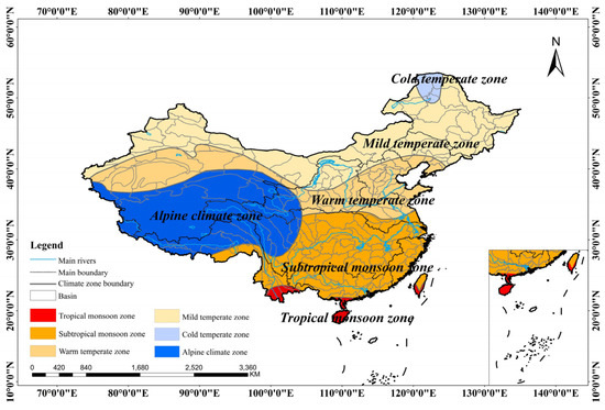
Figure 1.
The distribution of 214 third-order watersheds across six climate zones in China.
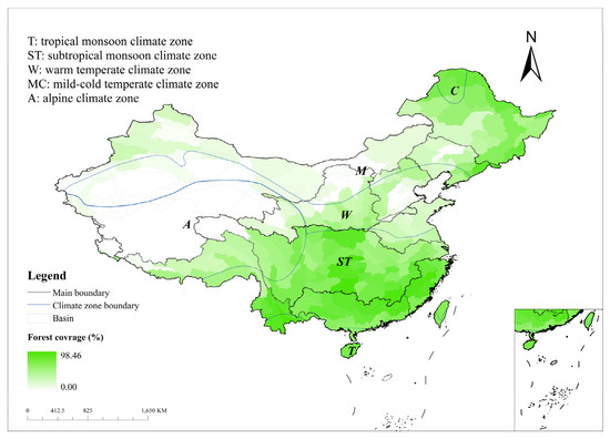
Figure 2.
The forest coverage in 214 watersheds across six climate zones in China.

Table 1.
The vegetation coverage across six climate zones in China.
2.2. Data
The GRACE Level-2 products provided by the Centre for Space Research (CSR) at the University of Texas (UTCSR: http://www.csr.utexas.edu/datasets/) (accessed on 1 December 2020) were used to extract GRACE data covering China from 2004 to 2014 in this study. The existing C20 term, an index to express gravitational variations, was replaced by the C20 term obtained by Satellite Laser Ranging (SLR) to improve the accuracy of the estimations [42,43]. Given that the correlations between spherical harmonic coefficients of different orders in the GRACE products would lead to bandings in images, decorrelation was applied first to remove north–south stripes. Then, the Gaussian smoothing filter was used to reduce errors from high orders. Finally, we applied the method recommended by Wahr et al., 1998 to generate the 0.25° × 0.25° TWSAs images, where TWSAs in watersheds across six climate zones in China from 2004 to 2014 can be derived to perform the following analyses [44]. We applied high-frequency filtering and de-striping algorithms to reduce the noise level of GRACE data, which have been proven to be effective but would weaken the effective signal of the model [45,46,47]. The signal in the target region may leak into the surrounding areas and cause amplitude damping in the region (leakage-out). The signal from the surrounding areas may also leak into the target region (leakage-in). To address this issue, we used the signal leakage algorithm and applied the GRACE Matlab Toolbox (GRAMAT) to mitigate the effect of signal leakage. The toolbox was developed on the MacOSX operating systems with the Matlab software (version R2014a) by Feng Wei (Wuhan, China) [47]. Then, we applied the scaling method to downscale the resolution, which optimizes the basin shape descriptions. Existing studies [47,48,49] have indicated this method is suitable for retrieving TWS for small basins.
Monthly climate data with a spatial resolution of 0.5°, including precipitation, evapotranspiration, and mean temperature, were collected from Chinese Surface Climate Information of the National Meteorological Information Center (http://www.nmic.cn/) (accessed on 1 February 2021). Effective precipitation (PE), which refers to the precipitation that is available for the generation of surface water, was calculated as the difference between precipitation (P) and evapotranspiration (ET) by Equation (1) [50].
PE = P − ET
Three types of vegetation data including the leaf area index (LAI), normalized difference vegetation index (NDVI), and vegetation fraction coverage (VFC) were used to describe vegetation conditions. LAI data were derived from the Global Land Surface Satellite LAI (GLASS LAI) product provided by the National Earth System Science Data Center (http://www.geodata.cn) (accessed on 5 February 2021), with a spatial resolution of 0.05°. NDVI was obtained from the Global Inventory Modelling and Mapping Studies (GIMMS) NDVI 3 g dataset at a temporal resolution of 15 days and a spatial resolution of 1/12° (http://poles.tpdc.ac.cn/en/data/9775f2b4-7370-4e5e-a537-3482c9a83d88/) (accessed on 5 February 2021). VFC was calculated based on NDVI (Equation (2)).
VFC = (NDVI − NDVImin)/(NDVImax − NDVImin)
To describe watershed characteristics, we also used soil moisture and land cover data. The soil moisture data were derived from the Global Land Data Assimilation System (GLDAS) dataset with a spatial resolution of 500 m (https://ldas.gsfc.nasa.gov/gldas) (accessed on 10 February 2021). Land cover data were derived from the MODIS Land Cover Type Product (MCD12Q1) with a spatial resolution of 500 m (https://ladsweb.modaps.eosdis.nasa.gov/) (accessed on 10 February 2021).
Human activities data were derived from the China National Bureau of Statistics (http://www.stats.gov.cn/) (accessed on 1 March 2021) and WorldPop (https://www.worldpop.org/) (accessed on 5 March 2021). The former dataset provided human activities data of each province including the Gross Domestic Product (GDP), per capita GDP, irrigated area, water consumption for industrial, agricultural, and domestic activities, and total water consumption, while the latter had annual population density data with a spatial resolution of 1km. To calculate watershed-scale human activity data, we firstly derived gridded-based population density at the watershed and province scale from WorldPop, respectively, to calculate the population density ratio (pi) for each watershed (Equation (3)). Then, we calculated human activity data for each watershed (Ai) according to human activity data at the province scale (A) and pi (Equation (4)).
where pi, PDi, PD, Ai, and A denote the population density ratio, population density at the watershed scale, population density at the province scale, human activity data at the watershed scale, and human activity data at the province scale, respectively.
pi = PDi/PD
Ai = pi × A
2.3. Methods
This study was designed to identify TWS dynamics and associated driving factors in watersheds across six climate zones in China (Figure 3). Firstly, the potential driving factors for watershed TWS were classified into three types: Climate, watershed characteristics, and human activities, which were widely used in existing studies [51,52,53,54,55,56,57,58,59]. The selected climate factors include annual precipitation (P), effective precipitation (PE), evapotranspiration (ET), and annual mean temperature (Tave). Soil moisture (SM) and vegetation indices including LAI, NDVI, and VFC were selected to represent watershed characteristics for TWS variations, while factors such as water use by agriculture, industry, and domestic activities, population density, and GDP were selected to express human influences. Detailed information on drivers can be found in Table 2.
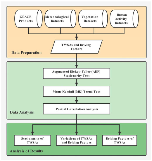
Figure 3.
Research design.

Table 2.
The summary of driving factors for watershed TWS.
The augmented unit root test (ADF test) proposed by Dickey and Fuller was then used to test the stationarity of each time series of data, which can indicate the inter-annual variations of TWS [60,61]. In the ADF test, the stationarity is evaluated based on the absolute value of the characteristic roots [60,62]. If the t statistic is less than that of a given percentage level (e.g., 10% level) and the probability is greater than 0.10, the time series is non-stationary [63]. The non-parametric Mann–Kendall (MK) trend test was applied to detect the statistical significance of trends in data series, e.g., TWSAs for each study watershed from 2004 to 2014 with a significance level of 0.05 [64,65,66]. The partial correlation analysis was finally adopted in this study to detect the correlations between TWSAs and driving factors at a statistically significant 0.05 level, which can indicate the key factors for TWS variations, as well as the associated driving mechanisms [51].
3. Results
3.1. TWSAs and Driving Factors: Trend and Stationarity
3.1.1. Trends and Stationarities of TWSAs
As suggested by ADF and MK tests (Table 3 and Table 4), TWSAs for 214 watersheds from 2004 to 2014 are non-stationary (t = −2.59 and Prob. > 0.10) with a significant downward trend (Z = −3.62 and p < 0.05). Although the time series of TWSAs are non-stationary in watersheds from all climate zones, the change patterns of TWSAs differ among climate zones. From 2004 to 2014, there are significant increasing trends (p < 0.05) in TWSAs in tropical and subtropical watersheds, and significant decreases in TWSAs (p < 0.05) in warm temperate and alpine watersheds. An insignificant trend is detected in watersheds from the mild-cold temperate zone.

Table 3.
Results of trends in TWSAs from 2004 to 2014.

Table 4.
Results of stationarity tests in TWSAs.
3.1.2. Trends of Driving Factors
Figure 4 exhibits the results of trend tests for driving factors from 2004 to 2014. Significant increasing trends are detected in NDVI, GDP, PERGDP, WT, and IRR (p < 0.05) for all watersheds. Specifically, ET, LAI, NDVI, VFC, IND, GDP, PERGDP, IRR, and PD significantly increase in tropical watersheds. For subtropical watersheds, there are significant increments in ten driving factors (i.e., P, PE, ET, Tave, LAI, NDVI, VFC, DW, GDP, and PERGDP). Significant increments are found in the AGR, WT, GDP, PERGDP, and IRR in watersheds in the mild-cold temperate climate zone. Similarly, significant upward trends are detected in AGR, GDP, PERGDP, and IRR in watersheds in the alpine climate zone. Additionally, a significant decreasing trend is observed in soil moisture (SM), while significant increasing trends are tested in GDP and PERGDP in the warm temperate watersheds.
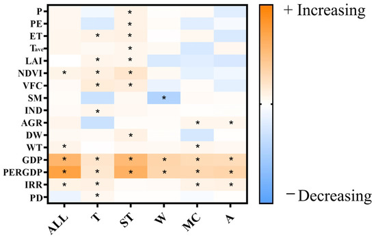
Figure 4.
Trend tests of driving factors from 2004 to 2014. * Significant at α = 0.05. T, ST, W, MC, and A denote tropical monsoon, subtropical monsoon, warm temperate, mild-cold temperate, and alpine climate zones, respectively.
3.2. Spatial Variations of TWSAs
The spatial pattern of trends in TWS is distinct across climate zones. Significant upward (p < 0.05) trends in TWSAs mostly appear in watersheds located in the tropical monsoon, subtropical monsoon, and northern alpine climate zones, while significant downward trends of TWSAs are often found in watersheds in the warm temperate, southern alpine, and western mild-cold temperate climate zones (Figure 5).
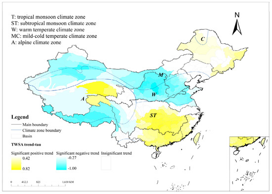
Figure 5.
TWSAs trends from 2004 to 2014 in 214 watersheds in China (p < 0.05).
3.3. Spatial Variations of Vegetation Change
Changes in forest and grassland are widespread from 2004 to 2014 in China. According to Figure 6a, significant upward trends (p < 0.05) in forest coverage are mainly found in tropical, western subtropical, central warm temperate, and eastern mild-cold temperate watersheds, while significant declines (p < 0.05) are found in watersheds located in the eastern subtropical climate zones. Grassland coverage shows significant and rising tendencies (p < 0.05) in watersheds located in the western warm or mild temperate (e.g., Tarim Basin), northern alpine, and the eastern subtropical climate zones, whereas significant and decreasing tendencies (p < 0.05) are shown in the eastern alpine (e.g., Qaidam Basin and headwater sources of the Yangtze and Yellow Rivers), southwestern subtropical, central warm temperate (particularly the Loess Plateau), and the cold temperate climate zones (Figure 6b). Changes in shrubland were generally limited across six climate zones without a distinct pattern (Figure 6c).
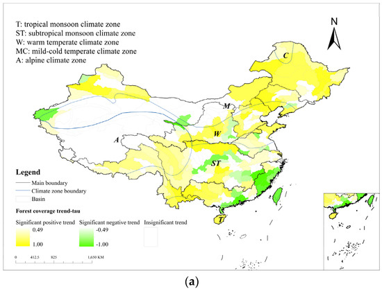
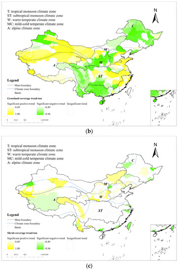
Figure 6.
(a) Forest coverage trends from 2004 to 2014 in 214 watersheds in China (p < 0.05); (b) grassland coverage trends from 2004 to 2014 in 214 watersheds in China (p < 0.05); (c) shrub coverage trends from 2004 to 2014 in 214 watersheds in China (p < 0.05).
3.4. Key Driving Factors for TWSAs in Different Climate Zones
Climate, watershed characteristics, and human activities can significantly affect TWSAs (Figure 7). As suggested by partial correlation analysis, for 214 watersheds in China, significant positive correlations are observed between TWSAs and P, PE, NDVI, and SM, whereas significant negative correlations are found between TWSAs and ET, Tave, IRR, AGR, DW, and WT (p < 0.05). Watersheds from each climate zone feature different key driving factors for TWSAs. In tropical monsoon watersheds, significant positive relationships are observed between TWSAs and P, NDVI, and SM while significant negative relationships between TWSAs and ET, Tave, and WT are identified. In subtropical watersheds, TWSAs significantly increase with increasing P, PE, NDVI, and SM, but decrease with increasing ET, Tave, AGR, and WT. In warm temperate watersheds, TWSAs are positively correlated with P, LAI, NDVI, and SM, but negatively correlated with ET, Tave, and human activities (i.e., IRR, IND, AGR, WT, GDP, and PERGDP). For watersheds in the mild-cold temperate zone, there are significant and positive relationships between TWSAs and P, PE, NDVI, and SM but significant and negative relationships between TWSAs and ET, Tave, LAI, VFC, IND, AGR, WT, and GDP. In addition, TWSAs are positively related to P, PE, NDVI, and SM, but negatively correlated with ET, Tave, IRR, AGR, and WT in alpine watersheds.
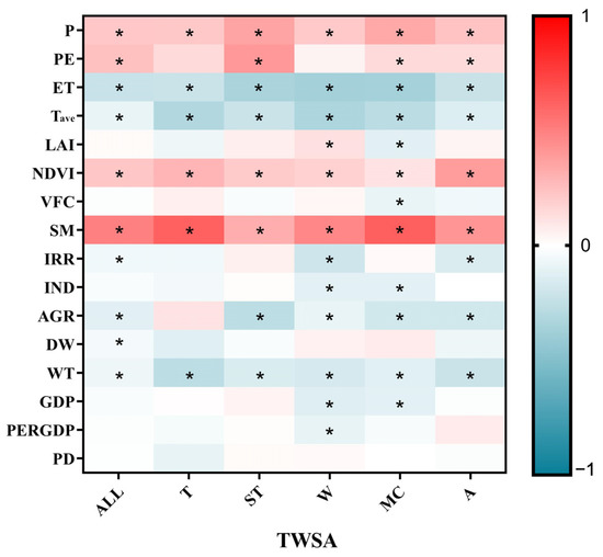
Figure 7.
The partial correlations between TWSAs and their driving factors. T, ST, W, MC, and A represent tropical monsoon, subtropical monsoon, warm temperate, mild-cold temperate, and alpine climate zones, respectively. (* Significant at α = 0.05).
4. Discussion
4.1. The Dynamics of Terrestrial Water Storage and Their Driving Factors across Climate Zones
Our study clearly indicates that TWS in China was non-stationary and significantly changed (Table 3 and Table 4 and Figure 5) by climate variability, vegetation change, and anthropogenic activities from 2004 to 2014 (Figure 7, Figure A3, Figure A4 and Figure A5). Overall, TWSAs show significant downward trends mostly in watersheds in warm temperate, southern alpine, and western mild-cold temperate climate zones during the study period (Figure 5), mainly resulting from intense human activities (i.e., changes in WT and IRR), while significant upward (p < 0.05) trends in TWSAs generally appear in watersheds from tropical monsoon, subtropical monsoon, and northern alpine climate zones possibly due to increased precipitation and forest coverage (Figure 6a). As suggested by Figure 4 and Figure A4b, NDVI has a significant increasing trend in China as a result of a series of vegetation restoration projects (e.g., the Grain for Grain Program and the Natural Forest Protection Program) since the 1990s, which could improve the water conservation capacity to some extent and may partly contribute to increasing TWSAs in watersheds covered by mature forest stands and well-established vegetation (Figure 6a and Figure 7) [67]. However, the positive impact of vegetation change on TWS can be offset by human activities, which can influence water storage immediately. Fast-growing demands for total water use (WT) and irrigation (IRR) have greatly aggravated water storage deficits (Figure 4, Figure 7 and Figure A5d,e), especially in semi-arid and arid watersheds, resulting in significant declines in TWSAs during the study period [68,69,70]. For example, Wang et al. [68] found that strongly decreasing trends occurred in surface water and TWS in China from 1989 to 2016.
Nevertheless, TWS dynamics and associated driving factors vary among watersheds from different climate zones. In tropical watersheds, vegetation and climate play important roles in modulating TWS, where P, ET, Tave, NDVI, SM, and WT are identified as significant drivers for TWS variations (Figure 7). However, only ET and forest coverage have significant upward trends in tropical watersheds (Figure 4, Figure 6a and Figure A3c), which could be the determinant for the increased TWSAs during the study period. As is known, well-established vegetation covers often play an important role in regulating streamflow, soil moisture, and water retention capacities in ecosystems, which serve as the crucial link between below-ground and above-ground ecohydrological processes [71]. On the one hand, vegetation can increase recharges for groundwater, baseflow, and soil moisture by various hydrological processes such as interception and soil infiltration [72], which is favorable for below-ground TWS. On the other hand, vegetation growth is associated with increased ET, which would decrease surface and total streamflow [31], and thus decrease TWSAs (Figure 7). Given that tropical natural forests often have greater water retention capacities with complex forest structures, which are beneficial for maintaining water resources [73,74], a significant water surplus is expected in tropical watersheds once the increments in below-ground water storage outweigh the above-ground ET losses by forest growth.
In subtropical watersheds, climate and vegetation are also the main contributors to the increased TWS over the study period. A large number of subtropical watersheds have significantly increased forest coverage and NDVI (Figure 6a and Figure A4b) due to afforestation and reforestation. The well-established forest stands can intercept rainfall through the canopy, reducing the raindrop velocity and protecting surface soil [75]. Moreover, forests are characterized by deep rooting systems that can promote infiltration, recharge baseflow and groundwater, and mitigate soil erosion, which could eventually increase TWSAs. In addition, significant increments in precipitation and effective precipitation also contribute to TWSA increases (Figure 4 and Figure 7) in these subtropical watersheds, although rising ET and Tave may offset the increase in TWS caused by vegetation and precipitation increase (Figure 4, Figure 7 and Figure A3c,d). Besides, although TWSAs are significantly related to WT and AGR in a negative way (Figure 7), these two anthropogenic drivers show insignificant changes during the study period, and thus yield limited contributions to TWS in subtropical watersheds.
The decreasing tendency in TWS over the study period is widespread in warm temperate watersheds (Figure 5), which largely corresponds to significant declines in soil moisture (Figure 4), especially in watersheds located in the North China Plain and the northern Loess Plateau (Figure A4d). In addition, intensive human activities with fast-growing water use by agriculture (e.g., AGR and IRR) and urban development (e.g., IND, DW, and WT) (Figure 7 and Figure A5) are also the main contributors to the decreased TWS in warm temperate watersheds. Moreover, the declines in TWS can be aggravated by vegetation loss (e.g., the clearance of grass and forest) as a result of settlement development and agricultural expansion, especially in some watersheds in the North China Plain [76] where grassland degradation (Figure 6b) due to urbanization, agricultural expansion, and groundwater exploitation (Figure A5) is widespread. The negative impact of human activities on TWS can sometimes even override the positive effect of precipitation and vegetation on TWS. For example, increasing precipitation and vegetation in watersheds in the Loess Plateau would potentially increase TWS (Figure A3a and Figure A4a–c), while intense human activities offset the increments, eventually leading to a significant decline in TWS (Figure 5, Figure 7 and Figure A5). These indicate that most watersheds in the warm temperature climate zone have been confronted with growing water shortages due to excessive human activities over the study period, where water supply could be under much greater stress in the future with reduced precipitation under climate change.
In the alpine climate zone, significant declines in TWS are detected in watersheds in the southern and southeastern Qinghai–Tibet Plateau, while increasing TWS are observed in watersheds in the Qaidam Basin and headwater sources of the Yangtze River. Watersheds in the alpine climate zone are very sensitive to climate change given their large area of frozen soils, permanent snows, and glaciers. TWS variations in these watersheds are mainly controlled by climate and climate-induced vegetation change, such as agriculture activities, grazing, and cultivation (Figure A3a–d). For example, in the past 20–30 years, 38.8% of the grassland and nearly 50% of broad-leaf forest in the Qinghai–Tibet plateau were under degradation mainly due to climate change and grazing, which inevitably reduced TWS in this area [77,78]. Although precipitation significantly decreased over the study period in watersheds from the Qaidam Basin and headwater sources of the Yangtze River, the decreased LAI due to grassland degradation and the associated declines in ET and increases in soil moisture collectively led to significant increases in TWS in these watersheds (Figure 6b and Figure A4c,d). On the contrary, watersheds in the southern and southeastern Qinghai–Tibet Plateau are dominated by alpine forest, meadow, and glaciers with declined precipitation and soil moisture and increased ET and glaciers retreat due to global warming (Figure 6a–c, Figure A3 and Figure A4d). The reduced precipitation and increased ET and glacier loss are the major contributors to significant declines in TWS in these alpine watersheds, with complex responses of alpine forests and meadows to climate warming. In addition, growing agricultural activities may also contribute to reductions in TWS in the alpine forest-dominated southern Qinghai–Tibetan Plateau, but their negative effects on TWS were offset by climate change impact in the grassland-dominated northern Qinghai-Tibetan Plateau [79,80] (Figure 4, Figure 7 and Figure A5b).
TWS generally remains nonstationary and shows an insignificant trend during the study period in mild-cold temperate zone watersheds (Table 3 and Table 4), which is mainly caused by the differences in TWS trends and associated drivers across this climate zone (Figure 5). The downward tendency of TWS is mostly detected in watersheds located in the eastern mild temperate zone (e.g., the Inner Mongolia Plateau), which is mainly due to growing water use as a result of ambitious agriculture expansion (Figure 4 and Figure 7) and accelerated grassland degradation (e.g., grazing activities) (Figure 6b) over the study period. Contrarily, due to the increased precipitation and evapotranspiration, and decreased temperature and population density, an upward tendency in TWS is found in watersheds in the cold temperate zone (e.g., Xiaoxing’anling mountains) where boreal coniferous and deciduous broadleaf forests are dominant, as well as seasonally frozen soils. Increased LAI and associated increments in ET are caused by newly regenerated or planted young forests, and these trees would consume more water than old-growth trees [81,82]. However, a significant water surplus occurs since the climate change effect (significant increments in precipitation and effective precipitation, and increased soil water resulting from accelerated and advanced melting of frozen soils) outweighs the above-ground ET losses due to forest growth (Figure 4, Figure 7 and Figure A3).
Interestingly, TWS in watersheds in mild-cold climate zones is positively related to NDVI but negatively related to LAI and VFC. Although these vegetation indices are widely used for monitoring, analyzing, and mapping temporal and spatial variations in vegetation structure, and describing biophysical straits, the relationships between these indices are complex given their differences in definitions and data sources [52,53,54]. Firstly, NDVI and LAI may not always have positive correlations [83,84]. For example, Ma et al. [83] found that the observation angles directly determine the accuracy of LAI and NDVI estimations, where NDVI decreases with increasing observation angles while there is a large value in LAI. Danson et al. [84] also found that there was no significant relation between LAI and NDVI when the value of LAI is larger than 6 based on remotely sensed data. Secondly, NDVI usually increases with rising VFC when VFC is low. However, their relationship can be negative when VFC is high given that the NDVI value may converge to 1 [85]. Therefore, NDVI may have a saturation problem and be insensitive to vegetation change especially in these cold temperate watersheds with dense coniferous forests [86]. This indicates the usage of NDVI for vegetation change in these watersheds should be cautious.
4.2. Limitations and Uncertainties
There are some uncertainties and limitations in our study associated with the selection of indices, the study period, and the research method. These 16 indices were selected according to existing studies. To describe watershed characteristics, we only involve vegetation indicators and soil moisture, while other soil metrics (e.g., soil porosity and texture) and topographic and landscape indices may also have impacts on TWS [87,88]. Moreover, permanent water storage (e.g., glaciers) is an important component of TWS. In the context of global warming, the glaciers would melt and affect local and downstream TWS [17]. However, there is a lack of detailed data describing glacier dynamics and other watershed characteristics (e.g., soil, topography, and landscape). Second, although this study fills the research gap that assesses TWS dynamics at large spatial scales in China, the study period of our study is relatively short. Admittedly, the longer the study period allows us to capture more robust trends and spatial patterns as well as their associated mechanisms. Future assessment of TWS dynamics with a longer study period should be performed if more data are available. In addition, uncertainties may arise from data products provided by different sources. For example, although the GLASS LAI products have been widely used, they have some limitations, such as the high dependence on the quality of surface reflectance [89]. The spatial resolution of GRACE data may also cause uncertainty in retrieving TWS. For the 214 watersheds, we only have 20 watersheds with a size of less than 10,000 km2, and the effect of spatial resolution on retrieving TWS is limited. Assessing quantitative relationships between TWS dynamics and different drivers could largely improve our understanding of the relative contributions of drivers to TWS. However, the quantitative estimations are difficult to validate since there is a lack of field data and effective quantification methods. Thus, our study focuses on qualitative correlations between TWS dynamics and drivers. Future studies and field samplings are needed to validate the accuracy of data from different sources.
5. Conclusions
The dynamics of TWS and their driving factors at a relatively large scale are rarely evaluated in China. Our assessment demonstrated that China experienced water deficits over the period from 2004 to 2014. Climate variability, watershed characteristics, and anthropogenic activities can significantly affect TWS. We conclude that dominating factors of TWS dynamics across climate zones are different. Our study indicates that researchers need to identify the major contributing factors to TWS in their study areas and suggests that watershed management strategies should be designed for watersheds from different climate zones with a comprehensive understanding of their specific TWS dynamics and driving mechanisms.
Author Contributions
Data collection, H.W., S.D. and Y.X.; data analysis, S.D. and Y.H.; manuscript drafting, S.D. and Y.H.; research design, M.Z.; manuscript revision, M.Z., Y.H. and E.Y. All authors have read and agreed to the published version of the manuscript.
Funding
This research was funded by the Science Foundation for Distinguished Young Scholars of Sichuan Province (2022JDJQ0005), the National Natural Science Foundation of China (31770759), and the National Key Research and Development Program of China (2017YFC0505006).
Institutional Review Board Statement
Not applicable.
Informed Consent Statement
Not applicable.
Data Availability Statement
Not applicable.
Acknowledgments
We are thankful for the data support from the “National Earth System Science Data Center, National Science & Technology Infrastructure of China (http://www.geodata.cn) (accessed on 5 February 2021)“, and the GRACE Matlab Toolbox (GRAMAT) designed by Feng Wei. We are also grateful to the editor and two anonymous reviewers for their constructive suggestions on this paper.
Conflicts of Interest
The authors declare no conflict of interest.
Abbreviations
| Terrestrial water storage | TWS |
| Terrestrial water storage anomalies | TWSAs |
| Gravity Recovery and Climate Experiment | GRACE |
| Mann-Kendall | MK |
| Augmented Dickey-Fuller | ADF |
| Forest coverage | FC |
| Shrub coverage | SC |
| Grassland coverage | GC |
| Tropical monsoon zones | T |
| Subtropical monsoon zones | ST |
| Warm temperate zones | W |
| Mild temperate zones | M |
| Cold temperate zones | C |
| Alpine climate zones | A |
| Mild-Cold temperate zone | MC |
Appendix A
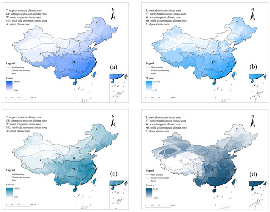
Figure A1.
The spatial distributions of long-term (a) P; (b) PE; (c) ET; and (d) Tave.
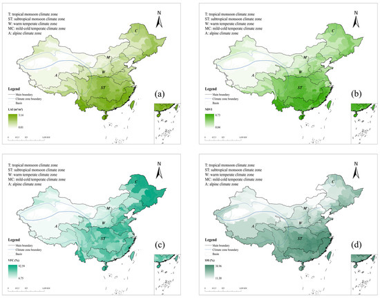
Figure A2.
The spatial distributions of long-term (a) LAI; (b) NDVI; (c) VFC; and (d) SM.
Appendix B
According to Figure A3a, significant increments (p < 0.05) in precipitation (P) are mainly detected in tropical, central warm temperate (particularly the Loess Plateau), and eastern mild-cold temperate watersheds, while significant decrements (p < 0.05) are found in watersheds located in alpine and eastern warm temperate climate zones. Effective precipitation (PE) significantly increases in warm temperate watersheds, whereas it significantly decreases in alpine and southwestern subtropical watersheds (Figure A3b). For significant changes in evapotranspiration (ET), most watersheds have increasing trends, while significant decrements in ET are identified in watersheds from northern subtropical and eastern warm temperate zones (Figure A3c). Additionally, temperature (Tave) shows significantly positive trends (p < 0.05) in watersheds in tropical, subtropical, alpine, warm, and western mild-cold temperate climate zones, while significantly negative variations (p < 0.05) occur in Northeast China experiencing the mild-cold temperate climate (Figure A3d).
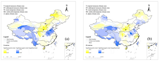
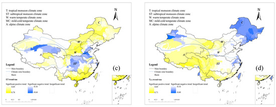
Figure A3.
The spatial distributions of significant temporal trends (p < 0.05) of (a) P; (b) PE; (c) ET; and (d) Tave.
Figure A4a suggests that LAI significantly increases (p < 0.05) in watersheds in tropical, subtropical, warm temperate, and mild-cold temperate climate zones. Significant increasing trends of NDVI are found in most study watersheds (Figure A4b). According to Figure A4c, significant increasing trends (p < 0.05) in VFC occur in alpine, subtropical, central warm temperate, and mild-cold temperate watersheds. For changes in SM (Figure A4d), significant upward trends (p < 0.05) are tested in tropical, southern subtropical, mild-cold temperate, and western warm temperate watersheds, while significant declines (p < 0.05) are observed in alpine and eastern warm temperate watersheds.
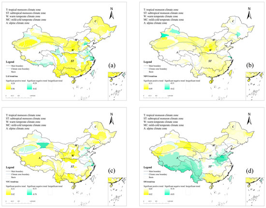
Figure A4.
The spatial distributions of significant change trends (p < 0.05) of (a) LAI; (b) NDVI; (c) VFC; and (d) SM.
The trend analysis indicates that industry water consumption (IND) undergoes significant increments (p < 0.05) in watersheds in mild-cold temperate, western alpine, and subtropical climate zones (Figure A5a). A significant upward trend (p < 0.05) in agricultural water use (AGR) is explored in watersheds located in the east and west of mild-cold temperate, alpine, central subtropical monsoon, and western warm temperate climates (Figure A5b). Compared with other climate zones, the changes in domestic water consumption (DW) significantly decrease in the south of alpine watersheds (Figure A5c). In addition, total water use (WT) has significant increasing trends (Figure A5d). In Figure A5e, there are markedly positive trends in irrigation area (IRR) in China except for watersheds in the central warm temperate climate zones. Lastly, there are significant decreasing trends in population density (PD) in watersheds located in the north of mild-cold temperate and the central subtropical monsoon climate zones, while other regions have significantly increasing PD (Figure A5f).
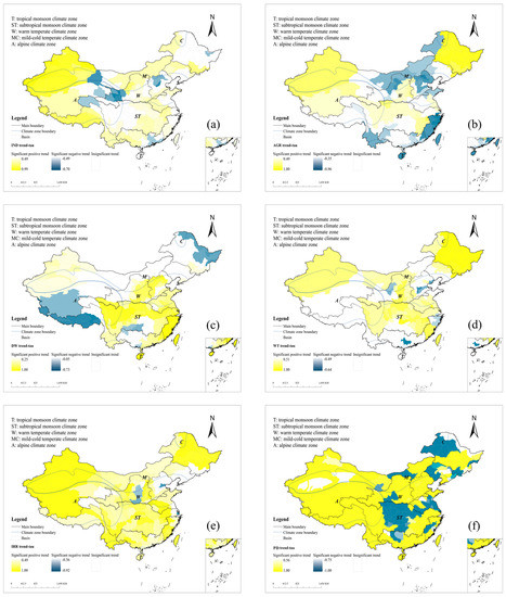
Figure A5.
The spatial distributions of significant change trends (p < 0.05) of (a) IND; (b) AGR; (c) DW; (d) WT; (e) IRR; and (f) PD.

Table A1.
Detailed information about watershed size, climate conditions, and TWS tends for 214 watersheds.
Table A1.
Detailed information about watershed size, climate conditions, and TWS tends for 214 watersheds.
| NO. | ID | Climate Zone | Area (km2) | P (mm) | Tave (°C) | TWS MK tau |
|---|---|---|---|---|---|---|
| 1 | A010100 | MC | 41,473.19 | 339.86 | 1.25 | 0.49 * |
| 2 | A010200 | MC | 58,611.51 | 437.43 | −0.66 | 0.45 * |
| 3 | A010300 | MC | 61,341.18 | 490.53 | −2.15 | 0.45 * |
| 4 | A020100 | MC | 69,452.51 | 566.96 | −0.13 | 0.42 * |
| 5 | A020200 | MC | 100,618.63 | 545.90 | 1.64 | 0.45 * |
| 6 | A020300 | MC | 138,267.04 | 520.10 | 4.21 | 0.42 * |
| 7 | A030100 | MC | 45,964.14 | 846.76 | 3.64 | 0.49 * |
| 8 | A030200 | MC | 33,667.01 | 688.09 | 4.91 | 0.31 |
| 9 | A040100 | MC | 32,730.16 | 652.25 | 4.18 | 0.27 |
| 10 | A040200 | MC | 64,548.34 | 648.47 | 2.99 | 0.38 |
| 11 | A040300 | MC | 41,242.49 | 700.78 | 2.43 | 0.42 |
| 12 | A040400 | MC | 44,987.73 | 675.08 | 1.82 | 0.49 * |
| 13 | A040500 | MC | 18,271.14 | 714.84 | 2.92 | 0.49 * |
| 14 | A050100 | MC | 123,785.80 | 620.06 | −0.65 | 0.42 |
| 15 | A060100 | MC | 24,845.07 | 679.86 | 2.79 | 0.56 * |
| 16 | A060200 | MC | 42,589.81 | 747.77 | 2.94 | 0.60 * |
| 17 | A070100 | MC | 11,441.55 | 691.30 | 2.44 | 0.60 * |
| 18 | A080100 | MC | 25,049.50 | 756.74 | 3.34 | 0.53 * |
| 19 | B010100 | W | 63,196.65 | 467.47 | 5.25 | 0.05 |
| 20 | B010200 | MC | 39,231.93 | 434.38 | 5.26 | 0.20 |
| 21 | B010300 | MC | 38,082.83 | 503.81 | 7.79 | 0.20 |
| 22 | B020100 | MC | 10,821.14 | 688.19 | 5.77 | 0.24 |
| 23 | B030100 | MC | 36,985.69 | 681.83 | 7.16 | 0.20 |
| 24 | B030200 | W | 14,168.27 | 690.43 | 8.72 | 0.27 |
| 25 | B040100 | W | 12,290.00 | 877.16 | 6.25 | 0.38 |
| 26 | B040200 | W | 16,747.98 | 875.84 | 6.65 | 0.42 |
| 27 | B050100 | MC | 24,471.30 | 982.81 | 3.72 | 0.53* |
| 28 | B050200 | W | 10,410.43 | 973.22 | 5.96 | 0.42 |
| 29 | B060100 | W | 26,227.84 | 856.18 | 7.91 | 0.24 |
| 30 | B060200 | W | 38,053.53 | 594.56 | 8.68 | 0.16 |
| 31 | C010100 | W | 45,043.11 | 530.77 | 6.49 | −0.27 |
| 32 | C010200 | W | 11,308.64 | 603.37 | 11.12 | −0.42 |
| 33 | C020100 | W | 22,293.76 | 546.10 | 8.43 | −0.56 * |
| 34 | C020200 | W | 17,729.95 | 445.14 | 6.22 | −0.85 * |
| 35 | C020300 | W | 28,154.55 | 477.38 | 6.32 | −0.78 * |
| 36 | C020400 | W | 16,277.47 | 541.11 | 12.20 | −0.64 * |
| 37 | C030100 | W | 18,829.10 | 495.42 | 9.46 | −0.82 * |
| 38 | C030200 | W | 12,962.85 | 518.92 | 13.11 | −0.78 * |
| 39 | C030300 | W | 13,998.49 | 525.19 | 13.17 | −0.75 * |
| 40 | C030400 | W | 31,242.82 | 522.33 | 9.23 | −0.89 * |
| 41 | C030500 | W | 15,424.85 | 558.94 | 14.16 | −0.89 * |
| 42 | C030600 | W | 26,510.46 | 582.60 | 10.40 | −0.82 * |
| 43 | C030700 | W | 9371.70 | 650.03 | 15.22 | −0.82 * |
| 44 | C030800 | W | 23,159.94 | 573.61 | 14.22 | −0.78 * |
| 45 | C040100 | W | 33,173.78 | 614.12 | 14.25 | −0.82 * |
| 46 | D010100 | A | 86,810.32 | 643.16 | −1.09 | 0.42 |
| 47 | D010200 | A | 45,624.64 | 510.67 | 0.96 | 0.31 |
| 48 | D020100 | A | 14,712.22 | 289.19 | −1.34 | −0.31 |
| 49 | D020200 | A | 16,408.75 | 350.02 | 3.51 | −0.31 |
| 50 | D020300 | A | 33,226.18 | 587.09 | 3.29 | −0.42 |
| 51 | D020400 | A | 26,522.28 | 407.34 | 4.21 | −0.38 |
| 52 | D030100 | A | 29,972.50 | 373.51 | 8.08 | −0.82 * |
| 53 | D030200 | W | 24,190.04 | 327.31 | 8.75 | −0.93 * |
| 54 | D030300 | MC | 31,760.93 | 238.31 | 9.84 | −0.96 * |
| 55 | D030400 | MC | 56,017.33 | 298.32 | 6.45 | −0.89 * |
| 56 | D030500 | MC | 21,255.23 | 301.16 | 8.44 | −0.89 * |
| 57 | D040100 | W | 39,045.65 | 452.61 | 8.48 | −0.93 * |
| 58 | D040200 | W | 23,669.62 | 394.27 | 8.71 | −0.93 * |
| 59 | D040300 | W | 48,479.81 | 420.97 | 10.01 | −1.00 * |
| 60 | D050100 | W | 40,106.59 | 528.62 | 9.07 | −0.89 * |
| 61 | D050200 | W | 24,996.79 | 504.66 | 9.67 | −0.82 * |
| 62 | D050300 | W | 43,799.44 | 486.02 | 9.49 | −0.82 * |
| 63 | D050400 | A | 31,078.78 | 554.87 | 7.40 | −0.75 * |
| 64 | D050500 | ST | 17,632.94 | 655.79 | 11.36 | −0.75 * |
| 65 | D050600 | ST | 18,413.12 | 664.77 | 12.52 | −0.78 * |
| 66 | D050700 | W | 16,102.14 | 644.92 | 12.63 | −0.75 * |
| 67 | D060100 | W | 6009.98 | 666.76 | 12.03 | −0.78 * |
| 68 | D060200 | W | 13,762.79 | 613.06 | 10.18 | −0.82 * |
| 69 | D060300 | ST | 18,918.75 | 711.46 | 12.22 | −0.71 * |
| 70 | D060400 | W | 3327.59 | 678.51 | 14.15 | −0.82 * |
| 71 | D070100 | W | 7570.86 | 676.30 | 15.32 | −0.82 * |
| 72 | D070200 | W | 11,520.84 | 699.17 | 13.12 | −0.82 * |
| 73 | D070300 | W | 4523.98 | 691.39 | 15.04 | −0.75 * |
| 74 | D080100 | MC | 43,524.95 | 285.24 | 8.71 | −0.93 * |
| 75 | E010100 | ST | 16,198.71 | 942.52 | 16.11 | −0.42 |
| 76 | E010200 | ST | 14,804.98 | 1028.58 | 16.03 | 0.05 |
| 77 | E020100 | ST | 67,661.97 | 828.15 | 15.47 | −0.78 * |
| 78 | E020200 | ST | 25,178.55 | 1122.53 | 15.77 | 0.05 |
| 79 | E020300 | ST | 31,742.58 | 889.09 | 15.50 | −0.82 * |
| 80 | E020400 | ST | 8401.70 | 1068.95 | 15.96 | −0.45 |
| 81 | E030100 | ST | 7851.87 | 1100.24 | 15.72 | −0.53 * |
| 82 | E030200 | ST | 25,017.33 | 1131.08 | 15.18 | −0.56 * |
| 83 | E040100 | W | 10,036.48 | 742.36 | 14.35 | −0.82 * |
| 84 | E040200 | W | 22,433.73 | 738.29 | 15.12 | −0.82 * |
| 85 | E040300 | W | 9751.93 | 838.77 | 14.65 | −0.82 * |
| 86 | E040400 | ST | 33,578.17 | 867.59 | 13.71 | −0.85 * |
| 87 | E040500 | W | 4179.98 | 843.47 | 13.33 | −0.82 * |
| 88 | E050100 | W | 14,550.42 | 680.76 | 13.43 | −0.82 * |
| 89 | E050200 | W | 48,336.09 | 744.74 | 12.52 | −0.53 * |
| 90 | F010100 | A | 146,040.82 | 408.21 | −3.91 | 0.60 * |
| 91 | F010200 | ST | 74,779.04 | 949.22 | 1.51 | −0.82 * |
| 92 | F020100 | ST | 12,8821.94 | 925.24 | 2.98 | −0.56 * |
| 93 | F020200 | ST | 12,8766.38 | 943.55 | 10.92 | −0.49 * |
| 94 | F030100 | ST | 77,155.92 | 937.02 | 2.90 | −0.27 |
| 95 | F030200 | ST | 58,696.32 | 935.55 | 9.22 | 0.05 |
| 96 | F030300 | ST | 27,132.36 | 955.36 | 17.28 | 0.49 * |
| 97 | F040100 | ST | 60,368.63 | 752.94 | 7.95 | −0.38 |
| 98 | F040200 | ST | 35,868.57 | 934.51 | 14.67 | 0.42 |
| 99 | F040300 | ST | 39,064.36 | 1017.61 | 15.51 | 0.42 |
| 100 | F040400 | ST | 23,800.93 | 966.02 | 16.77 | 0.38 |
| 101 | F050100 | ST | 51,083.17 | 1018.07 | 13.72 | 0.56 * |
| 102 | F050200 | ST | 36,997.82 | 1071.45 | 13.99 | 0.75 * |
| 103 | F060100 | ST | 19,092.87 | 940.97 | 14.56 | 0.49 * |
| 104 | F060200 | ST | 80,857.98 | 1054.45 | 15.53 | 0.71 * |
| 105 | F070100 | ST | 18,158.75 | 1211.08 | 14.69 | 0.75 * |
| 106 | F070200 | ST | 54,417.17 | 1180.79 | 15.36 | 0.78 * |
| 107 | F070300 | ST | 35,395.90 | 1200.50 | 15.33 | 0.78 * |
| 108 | F070400 | ST | 16,515.17 | 1272.79 | 16.04 | 0.82 * |
| 109 | F070500 | ST | 11,910.24 | 1277.88 | 15.74 | 0.78 * |
| 110 | F070600 | ST | 54,040.31 | 1360.81 | 17.15 | 0.75 * |
| 111 | F070700 | ST | 41,728.33 | 1343.38 | 17.48 | 0.78 * |
| 112 | F070800 | ST | 32,260.72 | 1262.03 | 17.29 | 0.75 * |
| 113 | F080100 | ST | 94,742.01 | 854.58 | 11.43 | −0.31 |
| 114 | F080200 | ST | 24,414.02 | 887.86 | 15.22 | −0.27 |
| 115 | F080300 | ST | 37,232.54 | 1059.64 | 15.33 | 0.53 * |
| 116 | F090100 | ST | 14,854.61 | 1432.96 | 16.08 | 0.75 * |
| 117 | F090200 | ST | 40,910.15 | 1547.86 | 17.74 | 0.67 * |
| 118 | F090300 | ST | 23,643.46 | 1472.95 | 17.60 | 0.71 * |
| 119 | F090400 | ST | 19,821.07 | 1468.32 | 17.65 | 0.78 * |
| 120 | F090500 | ST | 16,201.79 | 1601.23 | 17.60 | 0.67 * |
| 121 | F090600 | ST | 15,990.92 | 1688.19 | 16.99 | 0.64 * |
| 122 | F090700 | ST | 14,806.03 | 1574.38 | 16.99 | 0.67 * |
| 123 | F090800 | ST | 20,302.84 | 1497.02 | 17.66 | 0.75 * |
| 124 | F100100 | ST | 17,770.44 | 1154.60 | 12.72 | 0.78 * |
| 125 | F100200 | ST | 21,790.17 | 1142.38 | 16.20 | 0.71 * |
| 126 | F100300 | ST | 34,251.96 | 1158.87 | 16.54 | 0.49 * |
| 127 | F100400 | ST | 23,017.81 | 1325.82 | 16.93 | 0.71 * |
| 128 | F110100 | ST | 43,495.11 | 1236.87 | 16.18 | 0.20 |
| 129 | F110200 | ST | 35,552.60 | 1363.98 | 15.74 | 0.35 |
| 130 | F110300 | ST | 13,876.48 | 1306.54 | 15.89 | −0.35 |
| 131 | F120100 | ST | 17,820.64 | 1387.83 | 15.85 | 0.05 |
| 132 | F120200 | ST | 8436.70 | 1348.46 | 16.07 | −0.20 |
| 133 | F120300 | ST | 7742.61 | 1512.98 | 16.48 | 0.20 |
| 134 | F120400 | ST | 4757.13 | 1420.43 | 16.36 | −0.09 |
| 135 | G010100 | ST | 33,071.13 | 1696.34 | 15.77 | 0.56 * |
| 136 | G010200 | ST | 18,726.80 | 1661.86 | 15.61 | 0.35 |
| 137 | G020100 | ST | 10812.38 | 1722.91 | 16.31 | 0.27 |
| 138 | G020200 | ST | 1365.86 | 1782.27 | 0.00 | 0.36 |
| 139 | G030100 | ST | 15,229.00 | 1841.64 | 15.04 | 0.45 |
| 140 | G030200 | ST | 20,192.22 | 1865.49 | 15.53 | 0.42 |
| 141 | G040100 | ST | 17,009.52 | 1799.32 | 15.80 | 0.45 |
| 142 | G050100 | ST | 43,534.09 | 1676.38 | 16.65 | 0.60 * |
| 143 | G050200 | ST | 19,234.41 | 1730.08 | 16.85 | 0.53 * |
| 144 | G060100 | ST | 35,963.54 | 1693.45 | 18.26 | 0.60 * |
| 145 | G070100 | T | 38,877.74 | 1954.36 | 17.13 | 0.53 * |
| 146 | H010100 | T | 57,507.93 | 1028.04 | 15.03 | 0.05 |
| 147 | H010200 | ST | 26,572.96 | 1031.86 | 14.45 | 0.16 |
| 148 | H020100 | ST | 54,832.13 | 1280.75 | 18.08 | 0.56 * |
| 149 | H020200 | ST | 58,769.39 | 1300.93 | 17.29 | 0.60 * |
| 150 | H030100 | ST | 39,411.43 | 1281.92 | 17.29 | 0.53 * |
| 151 | H030200 | ST | 38,725.63 | 1570.26 | 19.11 | 0.71 * |
| 152 | H040100 | ST | 30,395.15 | 1508.51 | 18.60 | 0.67 * |
| 153 | H040200 | ST | 36,462.52 | 1731.22 | 20.60 | 0.67 * |
| 154 | H050100 | ST | 17,729.86 | 1529.82 | 17.79 | 0.75 * |
| 155 | H050200 | ST | 29,770.64 | 1692.95 | 19.16 | 0.75 * |
| 156 | H060100 | ST | 19,340.65 | 1724.52 | 19.16 | 0.67 * |
| 157 | H060200 | ST | 9089.74 | 1889.35 | 20.97 | 0.67 * |
| 158 | H070100 | ST | 7689.55 | 1955.68 | 20.74 | 0.71 * |
| 159 | H070200 | ST | 1124.95 | 1965.12 | 21.34 | 0.71 * |
| 160 | H070300 | ST | 19,514.04 | 1974.55 | 21.94 | 0.71 * |
| 161 | H070400 | ST | 24.89 | 1823.90 | 20.39 | 0.49 |
| 162 | H080100 | ST | 29,405.44 | 1673.25 | 18.84 | 0.64 * |
| 163 | H080200 | ST | 17,691.43 | 1736.14 | 20.52 | 0.67 * |
| 164 | H090100 | T | 34,093.06 | 1850.01 | 22.40 | 0.60 * |
| 165 | H090200 | T | 22,151.88 | 1770.85 | 21.67 | 0.60 * |
| 166 | H100100 | T | 34,122.92 | 2000.36 | 23.00 | 0.24 |
| 167 | H100200 | T | 46.77 | 1576.70 | 19.87 | 0.23 |
| 168 | J010100 | T | 23,648.34 | 1153.04 | 16.73 | 0.20 |
| 169 | J010200 | T | 36,858.42 | 1038.22 | 15.97 | −0.13 |
| 170 | J010300 | T | 15,475.56 | 1199.31 | 16.32 | 0.38 |
| 171 | J020100 | ST | 92,175.82 | 867.20 | 0.08 | −0.82 * |
| 172 | J020200 | T | 74,639.37 | 1209.03 | 16.20 | 0.13 |
| 173 | J030100 | ST | 109,419.77 | 856.71 | −1.04 | −0.82 * |
| 174 | J030200 | T | 24,578.61 | 1121.37 | 15.96 | −0.38 |
| 175 | J030300 | ST | 21,843.12 | 1224.27 | 12.50 | −0.53 * |
| 176 | J040100 | A | 57,856.28 | 677.61 | −4.39 | −0.85 * |
| 177 | J040200 | A | 148,406.72 | 825.84 | −0.95 | −0.93 * |
| 178 | J040300 | ST | 52,439.60 | 968.40 | 2.38 | −0.93 * |
| 179 | J050100 | ST | 151,638.00 | 1026.57 | 3.72 | −0.89 * |
| 180 | J060100 | A | 5622.61 | 238.17 | −11.39 | −0.49 * |
| 181 | J060200 | A | 59,445.04 | 465.36 | −4.96 | −0.89 * |
| 182 | K010100 | MC | 215,394.29 | 314.78 | 3.10 | 0.20 |
| 183 | K010200 | MC | 99,453.54 | 269.77 | 5.88 | −0.82 * |
| 184 | K020100 | A | 41,726.79 | 209.92 | 7.18 | −0.75 * |
| 185 | K020200 | A | 152,430.90 | 131.02 | 7.37 | −0.60 * |
| 186 | K020300 | A | 126,307.25 | 107.79 | 4.92 | −0.49 * |
| 187 | K020400 | W | 151,286.51 | 148.84 | 9.34 | −0.78 * |
| 188 | K030100 | A | 47,500.93 | 247.78 | −1.46 | 0.20 |
| 189 | K040100 | A | 78,565.45 | 216.56 | −1.46 | 0.67 * |
| 190 | K040200 | A | 202,154.52 | 118.15 | −0.17 | 0.82 * |
| 191 | K050100 | MC | 57,673.63 | 113.55 | 6.15 | −0.75 * |
| 192 | K050200 | W | 41,518.80 | 95.16 | 8.86 | −0.85 * |
| 193 | K050300 | W | 37,853.56 | 127.26 | 7.56 | −0.96 * |
| 194 | K060100 | MC | 50,693.78 | 276.03 | 1.81 | −0.16 |
| 195 | K060200 | MC | 26,241.70 | 215.73 | 4.42 | −0.38 |
| 196 | K060300 | MC | 8033.20 | 361.15 | 3.90 | −0.13 |
| 197 | K070100 | MC | 22,241.47 | 314.94 | 4.98 | −0.45 |
| 198 | K070200 | MC | 61,879.15 | 316.68 | 2.24 | −0.75 * |
| 199 | K080100 | MC | 88,652.18 | 208.83 | 8.03 | −0.64 * |
| 200 | K090100 | MC | 18,346.21 | 146.53 | 5.58 | −0.85 * |
| 201 | K090200 | MC | 85,909.97 | 243.12 | 4.99 | −0.75 * |
| 202 | K090300 | MC | 53,560.57 | 338.34 | 6.64 | −0.75 * |
| 203 | K100100 | A | 88,788.54 | 164.03 | 2.03 | −0.31 |
| 204 | K100200 | A | 98,125.46 | 255.45 | 1.77 | −0.49 * |
| 205 | K100300 | A | 87,948.13 | 298.22 | 3.96 | −0.49 * |
| 206 | K100400 | W | 54,636.34 | 262.86 | 6.65 | −0.60 * |
| 207 | K100500 | W | 41,588.46 | 196.08 | 6.65 | −0.75 * |
| 208 | K100600 | W | 111,173.19 | 119.92 | 4.58 | −0.89 * |
| 209 | K110100 | A | 73,358.80 | 107.87 | 7.36 | 0.02 |
| 210 | K110200 | A | 137,705.99 | 77.12 | 6.90 | 0.35 |
| 211 | K120100 | W | 33,832.29 | 122.80 | 5.39 | −0.85 * |
| 212 | K130100 | W | 234,953.07 | 110.99 | 13.63 | −0.64 * |
| 213 | K130200 | A | 134,052.61 | 74.68 | 11.06 | −0.75 * |
| 214 | K140100 | A | 791,638.02 | 277.51 | −5.13 | −0.47 * |
Note: T, ST, W, MC, and A denote tropical monsoon, subtropical monsoon, warm temperate, mild-cold temperate, and alpine climate zones, respectively. The positive values of MK tau denote increases in TWSAs, while negative values mean decreases. * Indicates significant at α = 0.05.
References
- Rodell, M.; Famiglietti, J.S. An analysis of terrestrial water storage variations in Illinois with implications for the Gravity Recovery and Climate Experiment (GRACE). Water Resour. Res. 2001, 37, 1327–1339. [Google Scholar] [CrossRef]
- Deng, H.J.; Pepin, N.C.; Liu, Q.; Chen, Y.N. Understanding the spatial differences in terrestrial water storage variations in the Tibetan Plateau from 2002 to 2016. Clim. Chang. 2018, 151, 379–393. [Google Scholar] [CrossRef]
- Kang, Z.; Nagel, P.; Pastor, R. Precise orbit determination for GRACE. Int. Space Geo. Syst. Sat. Dyn. 2003, 31, 1875–1881. [Google Scholar] [CrossRef]
- Gupta, D.; Dhanya, C.T. The potential of GRACE in assessing the flood potential of Peninsular Indian River basins. Int. J. Remote Sens. 2020, 41, 9007–9036. [Google Scholar] [CrossRef]
- Sinha, D.; Syed, T.H.; Famiglietti, J.S.; Reager, J.T.; Thomas, R.C. Characterizing Drought in India Using GRACE Observations of Terrestrial Water Storage Deficit. J. Hydrometeorol. 2017, 18, 381–396. [Google Scholar] [CrossRef]
- Seyoum, W.M.; Milewski, A.M. Improved methods for estimating local terrestrial water dynamics from GRACE in the Northern High Plains. Adv. Water Resour. 2017, 110, 279–290. [Google Scholar] [CrossRef]
- Yang, P.; Chen, Y.N. An analysis of terrestrial water storage variations from GRACE and GLDAS: The Tianshan Mountains and its adjacent areas, central Asia. Quatern. Int. 2015, 358, 106–112. [Google Scholar] [CrossRef]
- Dankwa, S.; Zheng, W.F.; Gao, B.; Li, X.L. Terrestrial Water Storage (TWS) Patterns Monitoring in the Amazon Basin Using Grace Observed: Its Trends and Characteristics. In Proceedings of the 2018 IEEE International Geoscience and Remote Sensing Symposium (IGARSS), Valencia, Spain, 22–27 July 2018; pp. 768–771. [Google Scholar] [CrossRef]
- Hu, Z.Y.; Zhang, Z.Z.; Sang, Y.F.; Qian, J.; Feng, W.; Chen, X.; Zhou, Q.M. Temporal and spatial variations in the terrestrial water storage across Central Asia based on multiple satellite datasets and global hydrological models. J. Hydrol. 2021, 596, 126013. [Google Scholar] [CrossRef]
- Wang, H.S.; Jia, L.L.; Steffen, H.; Wu, P.; Jiang, L.M.; Hsu, H.T.; Xiang, L.W.; Wang, Z.Y.; Hu, B. Increased water storage in North America and Scandinavia from GRACE gravity data. Nat. Geosci. 2013, 6, 38–42. [Google Scholar] [CrossRef]
- Pokhrel, Y.N.; Koirala, S.; Yeh, P.J.F.; Hanasaki, N.; Longuevergne, L.; Kanae, S.; Oki, T. Incorporation of groundwater pumping in a global Land Surface Model with the representation of human impacts. Water Resour. Res. 2015, 51, 78–96. [Google Scholar] [CrossRef]
- Famiglietti, J.S.; Lo, M.; Ho, S.L.; Bethune, J.; Anderson, K.J.; Syed, T.H.; Swenson, S.C.; de Linage, C.R.; Rodell, M. Satellites measure recent rates of groundwater depletion in California’s Central Valley. Geophys. Res. Lett. 2011, 38, L03403. [Google Scholar] [CrossRef]
- Humphrey, V.; Gudmundsson, L.; Seneviratne, S.I. Assessing Global Water Storage Variability from GRACE: Trends, Seasonal Cycle, Subseasonal Anomalies and Extremes. Surv. Geophys. 2016, 37, 357–395. [Google Scholar] [CrossRef]
- Hilker, T.; Lyapustin, A.I.; Tucker, C.J.; Hall, F.G.; Myneni, R.B.; Wang, Y.J.; Bi, J.; de Moura, Y.M.; Sellers, P.J. Vegetation dynamics and rainfall sensitivity of the Amazon. Proc. Natl. Acad. Sci. USA 2014, 111, 16041–16046. [Google Scholar] [CrossRef]
- Tobella, A.B.; Reese, H.; Almaw, A.; Bayala, J.; Malmer, A.; Laudon, H.; Ilstedt, U. The effect of trees on preferential flow and soil infiltrability in an agroforestry parkland in semiarid Burkina Faso. Water Resour. Res. 2014, 50, 3342–3354. [Google Scholar] [CrossRef]
- Taylor, R.G.; Scanlon, B.; Döll, P.; Rodell, M.; Van Beek, R.; Wada, Y.; Longuevergne, L.; Leblanc, M.; Famiglietti, J.S.; Edmunds, M.; et al. Ground water and climate change. Nat. Clim. Chang. 2013, 3, 322–329. [Google Scholar] [CrossRef]
- Rodell, M.; Famiglietti, J.S.; Wiese, D.N.; Reager, J.T.; Beaudoing, H.K.; Landerer, F.W.; Lo, M.H. Emerging trends in global freshwater availability. Nature 2019, 565, E7. [Google Scholar] [CrossRef]
- Frappart, F.; Papa, F.; da Silva, J.S.; Ramillien, G.; Prigent, C.; Seyler, F.; Calmant, S. Surface freshwater storage and dynamics in the Amazon basin during the 2005 exceptional drought. Environ. Res. Lett. 2012, 7, 044010. [Google Scholar] [CrossRef]
- Kuo, Y.N.; Lo, M.H.; Liang, Y.C.; Tseng, Y.H.; Hsu, C.W. Terrestrial Water Storage Anomalies Emphasize Interannual Variations in Global Mean Sea Level During 1997–1998 and 2015–2016 El Nino Events. Geophys. Res. Lett. 2021, 48, e2021GL094104. [Google Scholar] [CrossRef]
- Nie, N.; Zhang, W.C.; Guo, H.D.; Ishwaran, N. 2010–2012 drought and flood events in the Amazon Basin inferred by GRACE satellite observations. J. Appl. Remote Sens. 2015, 9, 096023. [Google Scholar] [CrossRef]
- Zhang, G.Q.; Yao, T.D.; Shum, C.K.; Yi, S.; Yang, K.; Xie, H.J.; Feng, W.; Bolch, T.; Wang, L.; Behrangi, A.; et al. Lake volume and groundwater storage variations in Tibetan Plateau’s endorheic basin. Geophys. Res. Lett. 2017, 44, 5550–5560. [Google Scholar] [CrossRef]
- Feng, W.; Zhong, M.; Lemoine, J.M.; Biancale, R.; Hsu, H.T.; Xia, J. Evaluation of groundwater depletion in North China using the Gravity Recovery and Climate Experiment (GRACE) data and ground-based measurements. Water Resour. Res. 2013, 49, 2110–2118. [Google Scholar] [CrossRef]
- Frederikse, T.; Landerer, F.; Caron, L.; Adhikari, S.; Parkes, D.; Humphrey, V.W.; Dangendorf, S.; Hogarth, P.; Zanna, L.; Cheng, L.J.; et al. The causes of sea-level rise since 1900. Nature 2020, 584, 393–397. [Google Scholar] [CrossRef] [PubMed]
- Zhang, Y.J.; Li, Y.; Ge, J.; Li, G.P.; Yu, Z.S.; Niu, H.S. Correlation analysis between drought indices and terrestrial water storage from 2002 to 2015 in China. Environ. Earth. Sci. 2018, 77, 462. [Google Scholar] [CrossRef]
- Zhang, Z.Z.; Chao, B.F.; Chen, J.L.; Wilson, C.R. Terrestrial water storage anomalies of Yangtze River Basin droughts observed by GRACE and connections with ENSO. Glob. Planet. Chang. 2015, 126, 35–45. [Google Scholar] [CrossRef]
- Scott, D.F.; Prinsloo, F.W. Longer-term effects of pine and eucalypt plantations on streamflow. Water Resour. Res. 2008, 44, W00A08. [Google Scholar] [CrossRef]
- Alila, Y.; Kuras, P.K.; Schnorbus, M.; Hudson, R. Forests and floods: A new paradigm sheds light on age-old controversies. Water Resour. Res. 2009, 45, W08416. [Google Scholar] [CrossRef]
- Woodsmith, R.D.; Vache, K.B.; McDonnell, J.J.; Helvey, J.D. Entiat Experimental Forest: Catchment-scale runoff data before and after a 1970 wildfire. Water Resour. Res. 2004, 40, W11701. [Google Scholar] [CrossRef]
- Sun, G.; Riekerk, H.; Kornhak, L.V. Ground-water-table rise after forest harvesting on cypress-pine flatwoods in Florida. Wetlands 2000, 20, 101–112. [Google Scholar] [CrossRef]
- Brown, A.E.; Zhang, L.; McMahon, T.A.; Western, A.W.; Vertessy, R.A. A review of paired catchment studies for determining changes in water yield resulting from alterations in vegetation. J. Hydrol. 2005, 310, 28–61. [Google Scholar] [CrossRef]
- Zhang, M.F.; Liu, N.; Harper, R.; Li, Q.; Liu, K.; Wei, X.H.; Ning, D.Y.; Hou, Y.P.; Liu, S.R. A global review on hydrological responses to forest change across multiple spatial scales: Importance of scale, climate, forest type and hydrological regime. J. Hydrol. 2017, 546, 44–59. [Google Scholar] [CrossRef]
- Li, Q.; Wei, X.H.; Zhang, M.F.; Liu, W.F.; Fan, H.B.; Zhou, G.Y.; Giles-Hansen, K.; Liu, S.R.; Wang, Y. Forest cover change and water yield in large forested watersheds: A global synthetic assessment. Ecohydrology 2017, 10, e1838. [Google Scholar] [CrossRef]
- Peng, X.P.; Fan, J.; Wang, Q.; Warrington, D. Discrepancy of sap flow in Salix matsudana grown under different soil textures in the water-wind erosion crisscross region on the Loess Plateau. Plant Soil 2015, 390, 383–399. [Google Scholar] [CrossRef]
- Wang, Y.Q.; Shao, M.A.; Zhu, Y.; Liu, Z. Impacts of land use and plant characteristics on dried soil layers in different climatic regions on the Loess Plateau of China. Agric. For. Meteorol. 2011, 151, 437–448. [Google Scholar] [CrossRef]
- Zhang, M.F.; Wei, X.H. Deforestation, forestation, and water supply A systematic approach helps to illuminate the complex forest-water nexus. Science 2021, 371, 990–991. [Google Scholar] [CrossRef]
- Ahmed, M.; Sultan, M.; Wahr, J.; Yan, E. The use of GRACE data to monitor natural and anthropogenic induced variations in water availability across Africa. Earth Sci. Rev. 2014, 136, 289–300. [Google Scholar] [CrossRef]
- Huo, Z.L.; Feng, S.Y.; Kang, S.Z.; Li, W.C.; Chen, S.J. Effect of climate changes and water-related human activities on annual stream flows of the Shiyang river basin in and north-west China. Hydrol. Process 2008, 22, 3155–3167. [Google Scholar] [CrossRef]
- Chen, Z.; Wang, W.J.; Jiang, W.G.; Gao, M.L.; Zhao, B.B.; Chen, Y.W. The Different Spatial and Temporal Variability of Terrestrial Water Storage in Major Grain-Producing Regions of China. Water 2021, 13, 1027. [Google Scholar] [CrossRef]
- Su, X.L.; Ping, J.S.; Ye, Q.X. Terrestrial water variations in the North China Plain revealed by the GRACE mission. Sci. China Earth Sci. 2011, 54, 1965–1970. [Google Scholar] [CrossRef]
- Yang, P.; Xia, J.; Zhan, C.S.; Wang, T.J. Reconstruction of terrestrial water storage anomalies in Northwest China during 1948–2002 using GRACE and GLDAS products. Hydrol. Res. 2018, 49, 1594–1607. [Google Scholar] [CrossRef]
- Qin, J.; Ding, Y.J.; Zhao, Q.D.; Wang, S.P.; Chang, Y.P. Assessments on surface water resources and their vulnerability and adaptability in China. Adv. Clim. Chang. Res. 2020, 11, 381–391. [Google Scholar] [CrossRef]
- Swenson, S.; Yeh, P.J.F.; Wahr, J.; Famiglietti, J. A comparison of terrestrial water storage variations from GRACE with in situ measurements from Illinois. Geophys. Res. Lett. 2006, 33, L16401. [Google Scholar] [CrossRef]
- Deng, H.J.; Chen, Y.N. Influences of recent climate change and human activities on water storage variations in Central Asia. J. Hydrol. 2017, 544, 46–57. [Google Scholar] [CrossRef]
- Wahr, J.; Molenaar, M.; Bryan, F. Time variability of the Earth’s gravity field: Hydrological and oceanic effects and their possible detection using GRACE. J. Geophs. Res.-Solid Earth 1998, 103, 30205–30229. [Google Scholar] [CrossRef]
- Klees, R.; Zapreeva, E.A.; Winsemius, H.C.; Savenije, H.H.G. The bias in GRACE estimates of continental water storage variations. Hydrol. Earth Syst. Sci. 2007, 11, 1227–1241. [Google Scholar] [CrossRef]
- Longuevergne, L.; Scanlon, B.R.; Wilson, C.R. GRACE Hydrological estimates for small basins: Evaluating processing approaches on the High Plains Aquifer, USA. Water Resour. Res. 2010, 46, W11517. [Google Scholar] [CrossRef]
- Feng, W. GRAMAT: A comprehensive Matlab toolbox for estimating global mass variations from GRACE satellite data. Earth Sci. Inform. 2019, 12, 389–404. [Google Scholar] [CrossRef]
- Rodell, M.; Velicogna, I.; Famiglietti, J.S. Satellite-based estimates of groundwater depletion in India. Nature 2009, 460, 999–1002. [Google Scholar] [CrossRef]
- Swenson, S.; Wahr, J. Multi-sensor analysis of water storage variations of the Caspian Sea. Geophys. Res. Lett. 2007, 34, L16401. [Google Scholar] [CrossRef]
- Stringham, T.K.; Snyder, K.A.; Snyder, D.K.; Lossing, S.S.; Carr, C.A.; Stringham, B.J. Rainfall Interception by Singleleaf Pinon and Utah Juniper: Implications for Stand-Level Effective Precipitation. Rangel. Ecol. Manag. 2018, 71, 327–335. [Google Scholar] [CrossRef]
- Zhang, Y.F.; He, B.; Guo, L.L.; Liu, J.J.; Xie, X.M. The relative contributions of precipitation, evapotranspiration, and runoff to terrestrial water storage changes across 168 river basins. J. Hydrol. 2019, 579, 124194. [Google Scholar] [CrossRef]
- Zhu, Z.C.; Bi, J.; Pan, Y.Z.; Ganguly, S.; Anav, A.; Xu, L.; Samanta, A.; Piao, S.L.; Nemani, R.R.; Myneni, R.B. Global Data Sets of Vegetation Leaf Area Index (LAI)3g and Fraction of Photosynthetically Active Radiation (FPAR)3g Derived from Global Inventory Modeling and Mapping Studies (GIMMS) Normalized Difference Vegetation Index (NDVI3g) for the Period 1981 to 2011. Remote Sens. 2013, 5, 927–948. [Google Scholar] [CrossRef]
- Gu, Z.J.; Ju, W.M.; Li, L.; Li, D.Q.; Liu, Y.B.; Fan, W.L. Using vegetation indices and texture measures to estimate vegetation fractional coverage (VFC) of planted and natural forests in Nanjing city, China. Adv. Space Res. 2013, 51, 1186–1194. [Google Scholar] [CrossRef]
- Pan, N.Q.; Feng, X.M.; Fu, B.J.; Wang, S.; Ji, F.; Pan, S.F. Increasing global vegetation browning hidden in overall vegetation greening: Insights from time-varying trends. Remote Sens. Environ. 2018, 214, 59–72. [Google Scholar] [CrossRef]
- Banerjee, C.; Sharma, A.; Kumar, D.N. Decline in terrestrial water recharge with increasing global temperatures. Sci. Total. Environ. 2021, 764, 142913. [Google Scholar] [CrossRef]
- Yan, J.B.; Jia, S.F.; Lv, A.F.; Mahmood, R.; Zhu, W.B. Analysis of the spatio-temporal variability of terrestrial water storage in the Great Artesian Basin, Australia. Water Supply 2017, 17, 324–341. [Google Scholar] [CrossRef]
- Deng, S.S.; Liu, S.X.; Mo, X.G. Assessment and attribution of China’s droughts using an integrated drought index derived from GRACE and GRACE-FO data. J. Hydrol. 2021, 603, 127170. [Google Scholar] [CrossRef]
- Zhou, M.L.; Wang, X.L.; Sun, L.; Luo, Y. Spatial Variations in Terrestrial Water Storage with Variable Forces across the Yellow River Basin. Remote Sens. 2021, 13, 3416. [Google Scholar] [CrossRef]
- Jing, W.L.; Yao, L.; Zhao, X.D.; Zhang, P.Y.; Liu, Y.X.Y.; Xia, X.L.; Song, J.; Yang, J.; Li, Y.; Zhou, C.H. Understanding Terrestrial Water Storage Declining Trends in the Yellow River Basin. J. Geophys. Res-Atmos. 2019, 124, 12963–12984. [Google Scholar] [CrossRef]
- Dickey, D.A.; Fuller, W.A. Distribution of the Estimators for Autoregressive Time Series with a Unit Root. J. Am. Stat. Assoc. 1979, 74, 427–431. [Google Scholar] [CrossRef]
- Dickey, D.A.; Fuller, W.A. Likelihood Ratio Statistics for Autoregressive Time Series with a Unit Root. Econometrica 1981, 49, 1057–1072. [Google Scholar] [CrossRef]
- Yu, E.X.; Zhang, M.F.; Hou, Y.P. Assessing Environmental Quality Dynamics and its Response to Vegetation Change in the Upper Minjiang River Watershed by Modis and Spot Products. In Proceedings of the 2021 IEEE International Geoscience and Remote Sensing Symposium (IGARSS), Brussels, Belgium, 11–16 July 2021; pp. 6472–6475. [Google Scholar] [CrossRef]
- Aylar, E.; Smeekes, S.; Westerlund, J. Lag truncation and the local asymptotic distribution of the ADF test for a unit root. Stat. Pap. 2019, 60, 2109–2118. [Google Scholar] [CrossRef]
- Mann, H.B. Nonparametric test against trend. Econometrica 1945, 13, 245–259. [Google Scholar] [CrossRef]
- Kendall, M.G. Rank Correlation Methods, 2nd ed.; Hafner Publishing Company: New York, NY, USA, 1955. [Google Scholar]
- Shao, G.W.; Guan, Y.Q.; Zhang, D.R.; Yu, B.K.; Zhu, J. The Impacts of Climate Variability and Land Use Change on Streamflow in the Hailiutu River Basin. Water 2018, 10, 814. [Google Scholar] [CrossRef]
- Liu, Z.J.; Wang, J.Y.; Wang, X.Y.; Wang, Y.S. Understanding the impacts of ‘Grain for Green’ land management practice on land greening dynamics over the Loess Plateau of China. Land Use Policy 2020, 99, 105084. [Google Scholar] [CrossRef]
- Wang, X.X.; Xiao, X.M.; Zou, Z.H.; Dong, J.W.; Qin, Y.W.; Doughty, R.B.; Menarguez, M.A.; Chen, B.Q.; Wang, J.B.; Ye, H.; et al. Gainers and losers of surface and terrestrial water resources in China during 1989–2016. Nat. Commun. 2020, 11, 3471. [Google Scholar] [CrossRef]
- He, P.X.; Sun, Z.J.; Han, Z.M.; Ma, X.L.; Zhao, P.; Liu, Y.F.; Ma, J. Divergent Trends of Water Storage Observed via Gravity Satellite across Distinct Areas in China. Water. 2020, 12, 2862. [Google Scholar] [CrossRef]
- Xu, L.; Chen, N.C.; Zhang, X.; Chen, Z.Q. Spatiotemporal Changes in China’s Terrestrial Water Storage From GRACE Satellites and Its Possible Drivers. J. Geophys. Res.-Atmos. 2019, 124, 11976–11993. [Google Scholar] [CrossRef]
- Trautmann, T.; Koirala, S.; Carvalhais, N.; Guntner, A.; Jung, M. The importance of vegetation in understanding terrestrial water storage variations. Hydrol. Earth Syst. Sci. 2022, 26, 1089–1109. [Google Scholar] [CrossRef]
- Zhang, L.; Wang, J.M.; Bai, Z.K.; Lv, C.J. Effects of vegetation on runoff and soil erosion on reclaimed land in an opencast coal-mine dump in a loess area. Catena 2015, 128, 44–53. [Google Scholar] [CrossRef]
- Yu, Z.; Liu, S.R.; Wang, J.X.; Wei, X.H.; Schuler, J.; Sun, P.S.; Harper, R.; Zegre, N. Natural forests exhibit higher carbon sequestration and lower water consumption than planted forests in China. Glob. Chang. Biol. 2019, 25, 68–77. [Google Scholar] [CrossRef]
- Huang, L.; Liu, J.Y.; Shao, Q.Q.; Xu, X.L. Carbon sequestration by forestation across China: Past, present, and future. Renew. Sust. Energy Rev. 2012, 16, 1291–1299. [Google Scholar] [CrossRef]
- Zhang, L.; Xiao, L.C.; Xiao, B.C.; Habib, S. Spatial-temporal changes of NDVI and their relations with precipitation and temperature in Yangtze river basin from 1981 to 2001. Geo. Spat. Inf. Sci. 2010, 13, 186–190. [Google Scholar] [CrossRef]
- Yuan, R.Q.; Chang, L.L.; Gupta, H.; Niu, G.Y. Climatic forcing for recent significant terrestrial drying and wetting. Adv. Water Res. 2019, 133, 103425. [Google Scholar] [CrossRef]
- Zhang, Y.L.; Liu, L.S.; Bai, W.Q.; Shen, Z.X.; Yan, J.Z.; Ding, M.J.; Li, S.C.; Zhen, D. Grassland Degradation in the Source Region of the Yellow River. Acta Geog. Sin. 2006, 61, 3–14. (In Chinese) [Google Scholar] [CrossRef]
- Peng, J.; Liu, Z.H.; Liu, Y.H.; Wu, J.S.; Han, Y.A. Trend analysis of vegetation dynamics in Qinghai-Tibet Plateau using Hurst Exponent. Ecol. Indic. 2012, 14, 28–39. [Google Scholar] [CrossRef]
- Tian, Y.Y.; Jiang, G.H.; Zhou, D.Y.; Li, G.Y. Systematically addressing the heterogeneity in the response of ecosystem services to agricultural modernization, industrialization and urbanization in the Qinghai-Tibetan Plateau from 2000 to 2018. J. Clean. Prod. 2021, 285, 125323. [Google Scholar] [CrossRef]
- Wang, H.; Zhou, X.L.; Wan, C.G.; Fu, H.; Zhang, F.; Ren, J.Z. Eco-environmental degradation in the northeastern margin of the Qinghai-Tibetan Plateau and comprehensive ecological protection planning. Environ. Geol. 2008, 55, 1135–1147. [Google Scholar] [CrossRef]
- Zhao, A.Z.; Zhang, A.B.; Lu, C.Y.; Wang, D.L.; Wang, H.F.; Liu, H.X. Spatiotemporal variation of vegetation coverage before and after implementation of Grain for Green Program in Loess Plateau, China. Ecol. Eng. 2017, 104, 13–22. [Google Scholar] [CrossRef]
- Jian, S.Q.; Zhao, C.Y.; Fang, S.M.; Yu, K. Effects of different vegetation restoration on soil water storage and water balance in the Chinese Loess Plateau. Agr. For. Meteorol. 2015, 206, 85–96. [Google Scholar] [CrossRef]
- Ma, J.J.; Yuan, J.G. Relationship between NDVI, View Zenith Angle and LAI based on Model Simulation. Remote Sens. Technol. Appl. 2014, 29, 539–546. (In Chinese) [Google Scholar] [CrossRef]
- Danson, F.M.; Plummer, S.E. Red-Edge Response to Forest Leaf-Area Index. Int. J. Remote. Sens. 1995, 16, 183–188. [Google Scholar] [CrossRef]
- Gitelson, A.A.; Kaufman, Y.J.; Stark, R.; Rundquist, D. Novel algorithms for remote estimation of vegetation fraction. Remote Sens. Environ. 2002, 80, 76–87. [Google Scholar] [CrossRef]
- Zhang, J.; Ge, J.P.; Guo, Q.X. The relation between the change of NDVI of the main vegetational types and the climatic factors in the northeast of China. Acta Ecol. Sin. 2011, 21, 4. (In Chinese) [Google Scholar] [CrossRef]
- Mohamed, A.; Abdelrahman, K.; Abdelrady, A. Application of Time-Variable Gravity to Groundwater Storage Fluctuations in Saudi Arabia. Front. Earth Sci. 2022, 10, 873352. [Google Scholar] [CrossRef]
- Girotto, M.; De Lannoy, G.J.M.; Reichle, R.H.; Rodell, M. Assimilation of gridded terrestrial water storage observations from GRACE into a land surface model. Water Resour. Res. 2016, 52, 4164–4183. [Google Scholar] [CrossRef]
- Ma, H.; Liang, S.L. Development of the GLASS 250-m leaf area index product (version 6) from MODIS data using the bidirectional LSTM deep learning model. Remote Sens. Environ. 2022, 273, 112985. [Google Scholar] [CrossRef]
Publisher’s Note: MDPI stays neutral with regard to jurisdictional claims in published maps and institutional affiliations. |
© 2022 by the authors. Licensee MDPI, Basel, Switzerland. This article is an open access article distributed under the terms and conditions of the Creative Commons Attribution (CC BY) license (https://creativecommons.org/licenses/by/4.0/).