New Perspectives for LVL Manufacturing from Wood of Heterogeneous Quality—Part 2: Modeling and Manufacturing of Variable Stiffness Beams

Abstract

This paper presents a new strategy in the use of wood of heterogeneous quality for composing LVL products. The idea is to consider veneers representative of the resource variability and retain local stiffness information to control panel manufacturing fully. The placement of veneers is also no longer random as in the first part of this group of papers but optimized for the quality of veneers according to the requirement of bending stresses along the beam. In a four-point bending test arrangement, this means the high-quality veneer is concentrated in the center of the beam in the area between the loading points where the bending moments are the most important, and the low quality is located at the extremities. This initiates the creation of variable stiffness beams. This is driven by an algorithm developed and tested on representative veneer samples from the resource. Four LVL panels were manufactured by positioning the veneers in the same positions as in an analytical calculation model, which allowed the calculation of beam mechanical properties in four-point bending. The proposed optimization of LVL manufacturing from variable quality veneers should help for more efficient usage of forest resources. This optimization strategy showed notable gains for modeled and experimental mechanical properties, whether in terms of stiffness or strength. The analytical calculation of the local modulus of elasticity from modelized beams was satisfactory compared to the tests of the manufactured beams test results, allowing the reliability of the model for this property to be confirmed.

1. Introduction

The laminated veneer lumber (LVL) is a lamellar composite material made of veneers from the rotary-peeling process. This material has several advantages. First, unlike sawn timber, it allows for a better distribution of defects within the material to avoid defects superimposition and thus homogenizes them in the product. Second, it can allow optimizing the placement of veneers according to their quality depending on the product’s performance needs. This is a very important advantage, particularly on very heterogeneous woods in terms of density and number and size of defects, such as large Douglas-fir woods.

In the peeling industry, the sorting of veneers to differentiate their quality is usually performed according to appearance criteria (knot size, slots, resin pockets, etc.) based on EN 635-3 standard [1]. This classification is generally practiced by the intervention of cameras integrated on the panel-making line. In the first part of the series of articles [2], it was shown that local modeling of elastic properties from local fiber orientation and average density could establish quality sorting criteria, giving sorting results significantly different from the standard sorting method. Now, distributing this high-quality heterogeneity of veneers using their local mechanical properties to obtain the best possible performance of the material is a major issue. The scientific literature presents extensive work on the consideration of veneers of different quality in LVL. Until now, a number of works have been aimed at upgrading inexpensive or low-grade veneers with better quality veneers while maximizing the bending properties of the material. Different LVL stacking sequences mixing beech and poplar plies were also tested in edgewise bending by Burdulu et al. [3]. It is not surprising that the configuration with the greatest number of beech plies, the denser species, provided the best performance in terms of bending stiffness and strength. Chen et al. [4] also presented similar findings in a hybrid bamboo-poplar LVL. They also performed flatwise bending tests that highlighted the importance of veneer quality depending on their distance to neutral fiber in this configuration. Hybrid LVL was also tested in [5] with acacia mangium and rubberwood. This was exclusively done by varying the species according to the plies, showing improvements in flatwise bending stiffness and strength when more dense species were used. All these literature results dealt with sequencing different species or qualities of veneers in the thickness of LVL, but to the authors’ knowledge, the optimization of the distribution of veneers of heterogeneous qualities along the product length has never been done before. It can be useful when LVL is used as slender beams loaded in edgewise bending.

This article belongs to a group of papers, whose first one is [2], which is dedicated to the use of heterogeneous species, such as large French Douglas-fir, in LVL manufacturing. In this first paper, the determination of local veneer properties by fiber orientation measurement integrated into the peeling line and veneer density enabled the establishment of a criterion to classify them according to their expected mechanical quality. Batches of veneers from the same classes were used to compose virtual panels with a random positioning of veneers. Panels were then virtually cut into beams, which were analyzed according to their equivalent modulus of elasticity to conclude the influence of sorting on the mechanical properties of the lamellar product. The aim was to propose an innovative grading method based on physical–mechanical properties and not just defects observed visually as it is performed for plywood industry (EN 635-3 standard), in order to manufacture reliable structural products.

However, the disadvantage of this random positioning of veneers is if the mechanical properties are rather low on average, consequently the mechanical properties of the LVL material will be low too. The sorting of the veneers can solve this issue but could lead to poor yields. However, in a beam subjected to bending, the stress is not homogeneous; thus, homogenized beams are partly oversized. Therefore, beams could be actually produced with heterogeneous mechanical properties to optimize utilization of raw material: using rather low-quality veneers where stress is low and high-quality veneers where stress is high. Mixing veneer qualities in a LVL beam is a challenge in the development of structural materials, as it means in this present context to consider the variability of the Douglas-fir resource to create beams with the highest possible mechanical properties.

The objectives of the present paper are multiple. First, a new strategy in the use of wood of heterogeneous quality for composing LVL products will be presented, enabling the quality of veneers to be optimized according to the requirement of bending stresses along the beam. This optimization is driven by a declination of a random veneer positioning panel manufacturing algorithm presented in [2]. Second, optimized panels were manufactured from a sample of veneers representative of the considered resource and were tested experimentally according to applicable standards [6,7]. The aim was both to draw conclusions on the model accuracy and to be able to estimate the performance of optimized beams realistically. In addition, to estimate the gains and losses in the mechanical properties of the optimized beams. Random beams from the same veneers were made numerically, simulating manufacturing without the view to optimizing panels. Finally, comparisons with beams from the different sorting methods from [2] were made so that the effects of grading could be estimated against the effects of optimized veneer placement.

2. Materials and Methods

First, this part explains how the veneers’ longitudinal modulus of elasticity was calculated in relation to Part 1 [2], taking into account possible variations in the relationship between modulus of elasticity and density. Then, the algorithm developed to optimize the longitudinal position of the veneers within the laminate according to their quality is presented. Finally, the experimental manufacturing of optimized panels is described, as well as the equations involved in the calculation of mechanical properties, determined experimentally and analytically.

Table 1. Nomenclature.

List of Main Symbols
$\overline{{\rho }_{veneer}}$	Averaged veneer density at 12% moisture content (kg·m−3);	$\overline{E_{veneer}}$	Averaged local modulus of elasticity on all veneer surface (MPa);
$\theta \left(x,y\right)$	Local fiber orientation angle (°);	$\overline{E_x}\left(x\right)$	Stiffness profile: averaged local modulus of elasticity along the length of veneer (MPa);
$\overline{E_{beam}}\left(x,y\right)$	Average of $E_{ply,n}\left(x,y\right)$ of the 15 constitutive plies (MPa);	$\overline{E_{x,panel}}\left(X\right)$	Sum of veneer $\overline{E_x}\left(x\right)$ profiles across panel width, averaged by the sum of flags at each X-position (MPa);
$E{I}_{eff}\left(x\right)$	Effective bending stiffness profile along the length of the beam (N mm2);	${\overline{E_x}}_{min}$	Stiffness profile minimum value (MPa);
$E{I}_{eff}{}_{min}$	Effective bending stiffness profile minimum value (N mm2);	$E_x\left(x,y\right)$	Local modulus of elasticity of veneer (MPa);
$E_{m,l,an}$	Analytical local modulus of elasticity in bending (MPa);	$f_{m,exp}$	Experimental bending strength (MPa);
$E_{m,l,exp}$	Experimental local modulus of elasticity in bending (MPa);	$\overline{H_{veneer}}$	Averaged normalized local Hankinson value on all veneer surface (dimensionless quantity);
$E_0$	Theoretical longitudinal elastic of modulus for straight grain (MPa);	MC	Moisture content (%);

contains the nomenclature listing the main symbols used.

2.1. Pollet Equations

The Pollet Equation [8] was the basis of the LVL beam analytical modeling process. Determined from a Douglas-fir mature, clear wood specimen, it allows the calculation of a bending elastic module from density information. In [2], the longitudinal modulus of elasticity in clear wood of the veneers was calculated using the average veneer density at 12% of moisture content (MC) according to Equation (1).

$$E_0=36.605\overline{{\rho }_{veneer}}-4242.4$$

(1)

where:

• E₀ is the theoretical elastic of modulus for straight grain (MPa) at 12% MC;
• $\overline{{\rho }_{veneer}}$ is the veneer average density (kg m⁻³) at 12% MC.

Then, the local fiber orientation regular grid was resized by applying a 12% MC tangential shrinkage coefficient [9]. Thus, the calculated mechanical properties of randomly composed beams were given at 12% MC to comply with convention.

In this paper, comparing the performance of manufactured LVL beams with modeled beams requires that veneer dimensions be consistent with their local fiber orientation regular grid. Indeed, material moisture content impacts these physico–mechanical properties (size, density, modulus of elasticity…) since the veneers were scanned in a green state, weighed after drying at 9% MC. Moreover, the beam moisture content was determined by double weighing small pieces of them during the destructive test [10], giving 7.5% MC for heartwood beams and 8% for sapwood ones. The Pollet equation (Equation (1)) requires 12% MC corrected density. Local longitudinal modulus of elasticity at 12% MC $E_x\left(x,y\right)$ was expressed from local fiber orientation regular grid resized in veneer width direction with a 7.5% (respectively 8%) MC tangential shrinkage coefficient for heartwood (respectively sapwood). Thus, the mechanical properties calculated from analytical tests were given at 12% MC. Concerning experimental moduli, they were corrected at 12% MC according to [11].

The experimental scatter used to calculate Equation (1) from this linear regression was very sparse, which raises the question of the accuracy of the formula. Thus, to consider the entire domain of potential modulus/density relationships, some declinations of it were calculated. The slope coefficients were all taken equal to the 36.605 m²s⁻² value of Equation (1), and several Y-intercept values were recalculated based on the percentage of points below each linear equation, as showed in Figure 1.

It means that, in the example of the 75% Pollet equation, the Y-intercept value was calculated in order that 75% of points were under the line.

Table 2. Pollet linear regression variants.

Percentage of Points under Line	Slope Coefficient	Y-Intercept	Stiffness Gain/Loss (MPa)
95%	36.605	−2140.1	+2102.3
75%		−3189.8	+1052.6
Initial equation		−4242.4	0
25%		−5408.8	−1166.4
5%		−7368.8	−3126.4

presents the coefficients of these equations. Thus, for example, the 75% Pollet equation implies +1052.6 MPa to add to the value of the longitudinal elastic modulus of clear wood.

The results from destructive tests presented afterward will be put into perspective with these equations to consider the sensitivity of Equation (1) in the mechanical properties prediction.

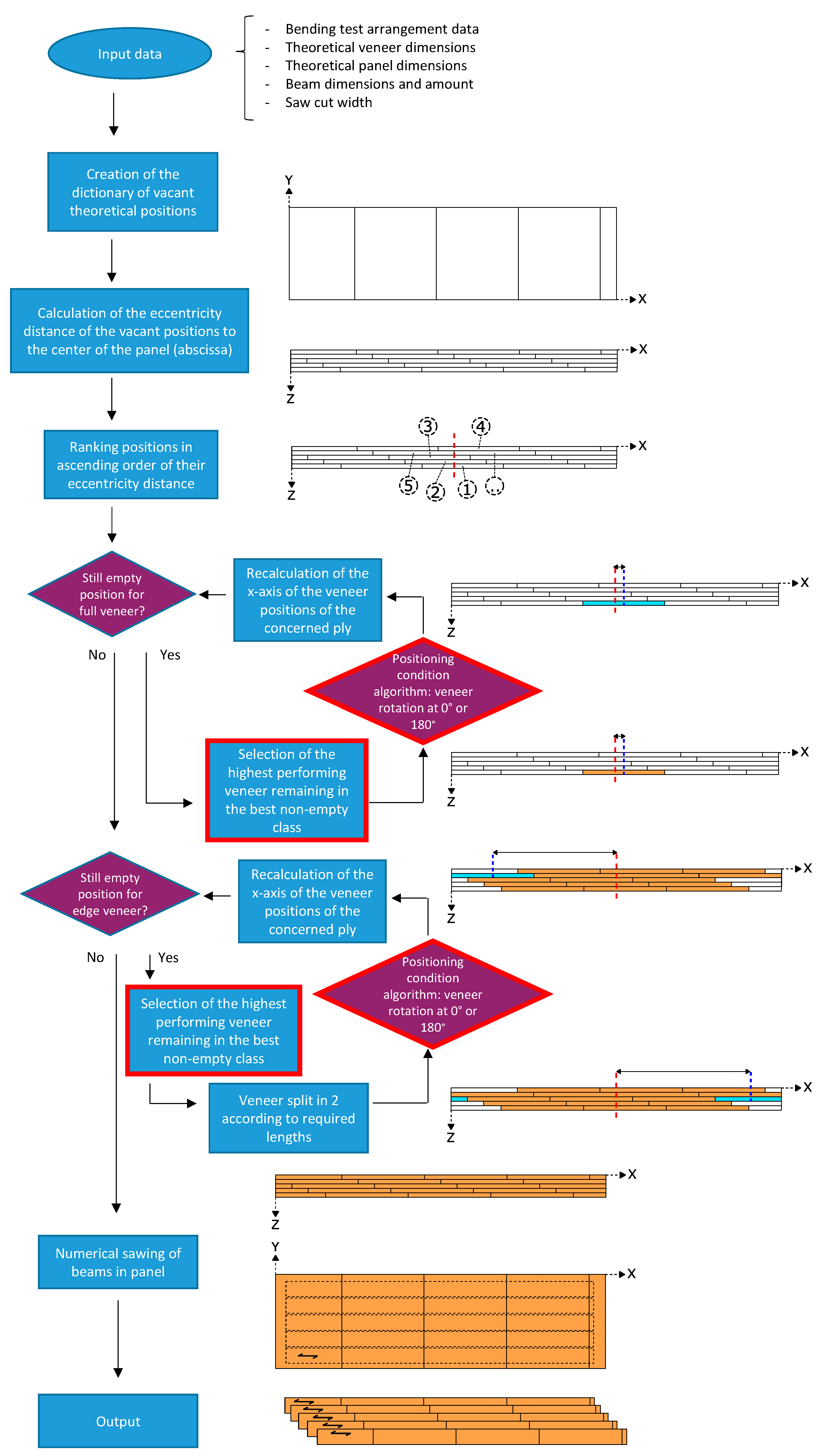
2.2. Favorable, Unfavorable, and Random Optimization Positioning

The presence of knots between loading points of the neutral axis creates zones of weakness that initiate failure. In addition, low density leads to low static bending strength [8]. The main objective was, therefore, to minimize the presence of zones of mechanical losses due to high knottiness and/or low density between loading points in a four-point bending configuration. The presence of knots in the beam area under tensile solicitation is critical, but this optimization was done in an undifferentiated manner between areas of compression and tensile in order to not limit by the direction of the beam in its use. A model for optimizing the distribution of veneers was developed to improve the mechanical properties of beams according to the bending stress imposed. The principle of optimizing the distribution proceeded by placing the veneers from the center of the panel towards the extremities and selecting the best performing veneer available on a defined criterion. The expected mechanical consequences were, therefore, better strength and higher local elastic moduli due to lower local grain angles in the beam area between the loading points.

Figure 2 is a flowchart describing the veneer-positioning algorithm, whose similarities can be observed with the functionality of the random placement algorithm presented in [2]. Boxes representing new functions are framed in red.

As in Part 1 [2], ($\overrightarrow{X}$, $\overrightarrow{Y}$) was the coordinate system of the panel. Each of these positions was initially considered as available. All vacant positions were first classified in ascending order according to their eccentricity distance (noted $X_{i,eccentricity,theo}$ in [2]). The first vacant position to be assigned was the one with the lowest absolute value of the eccentricity distance. Then, the highest-criterion veneer of the highest class was selected and allocated to this position. At this stage, the term criterion needed to be defined.

Here, the hierarchy between veneers of the same class was made according $\overline{E_{veneer }}$ value, defined in [2]. Each of the veneers was then picked to fill each of the vacant positions progressively. A feature of nonsuperposition of areas of low elastic modulus between plies was developed and added to avoid creating local mechanical weaknesses in the width of the material. The principle is explained in Figure 3. Each time a veneer was placed in a vacant position, a test was performed to choose between 0° or 180° to minimize defect superimposing. A sum of all stiffness profiles across the 15 plies between the X abscissa of the edges of the considered position (X_min and X_max) was performed. A flag system allowed this localized profile to be divided by the number of veneers allocated at this stage on the 15 plies on each X-axis coordinate between X_min and the X_max: its designation was $\overline{E_{x,panel}}\left(X\right)$. Then, the highest value found between the 2 cases dictated the positioning angle.

As in Part 1 [2] random algorithm, each time a veneer was allocated to a position, the theoretical abscissa of the vacant positions was recalculated from its real length. To simplify the algorithm, a veneer attributed to an end of ply was cut in half as required, and the second part completed the opposite ends. Again, for each one, the condition of no superimposing of defects was applied. Once all veneers had been assigned, and therefore all plies of the material panel were filled, numerical sawing of the beams in the panel was done according to the input setting dimension.

In order to put the mechanical results of the favorably optimized beams into perspective, the working principle of the algorithm previously described was reversed in order to also be able to create the opposite of favorably optimized beams. The principle of assigning positions in ascending order of eccentricity distance from the center of the panel was retained, but the choice by veneer performance was reversed. Veneers were selected and placed from worst to best quality according to prioritization criteria, the $\overline{E_{veneer }}$ value.

The Part 1 [2] numerical panel manufacturing algorithm by random veneer positioning was used too in order to evaluate the performance of optimized beams by generating panels and random beams. However, it was not possible to generate all the combinations of possible panels. Indeed, in this study, a panel was composed of 60 full veneers, divided into 72 positions considering veneers at extremities cut in half. Each veneer had two possible positions: 0° and 180°. In other words, there were 60! × 2⁷² = 3.93 × 10¹⁰⁰ possible combinations. Obviously, not all these configurations could be computer-generated in a reasonable time as it takes one minute per panel. For each batch of veneers, which were used to compose a panel, a sample of 150 combinations was generated per panel to allow some conclusions. A statistical test presented later will show that this hypothesis is relevant.

2.3. Panel Manufacturing and Samples Preparation

2.3.1. Composition of Representative Resource Batches

To allow for comparison of the mechanical results of the beams from heartwood and sapwood panels, a batch sampling of the 60 necessary veneers was conducted based on their individual $\overline{E_{veneer }}$ criterion. The objective was to obtain 2 batches of heartwood and 2 batches of sapwood veneers as similar as possible between them according to this criterion.

For this study, 4 optimized panels were composed:

-

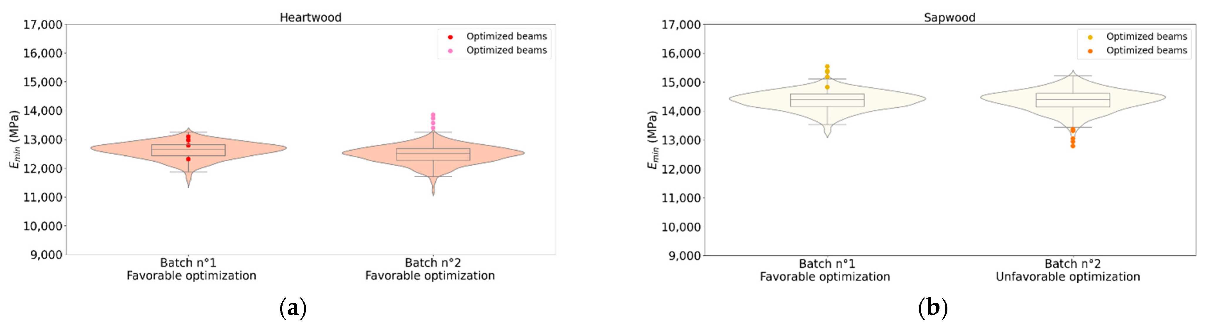
Heartwood batch n°1 veneers were used to manufacture a favorable veneer placement optimization without the “defect nonsuperposition” option: dense clear wood was concentrated in the middle of the panel;

-

Heartwood batch n°2 veneers were used to manufacture a favorable veneer placement optimization, with the “defect nonsuperposition” option: veneer positioning was driven by their quality and the homogenization of defects by the algorithm portion shown in Figure 3;

-

Sapwood batch n°1 veneers were used to manufacture a favorable veneer placement optimization without the “defect nonsuperposition” option: all available good quality wood veneers were concentrated in the center of the panel;

-

Sapwood batch n°2 veneers were used to manufacture an unfavorable veneer placement optimization: all available low-quality wood veneers were concentrated in the center of the panel, with the “defect superposition” option: in the final step of the algorithm in Figure 3, the lowest value of $\overline{E_{x,panel}\left(X\right)}$ was chosen to maximize the accumulation of areas of low mechanical property.

Once optimized (favorably or unfavorably), veneer positioning algorithms were used to build the panels, and a virtual cut-out of each beam in their actual dimensions and respecting placement in the real panel was performed.

In order to compare the sapwood and heartwood beams, respectively, the sampling of the veneers had to meet two requirements: the batches, representative of the initial resource, must have an overall equivalent population distribution by wood type. In practice, it is important to remember that this is impossible since each veneer is unique. To compose the veneer samples, the averaged local modulus of elasticity on all veneer surfaces $\overline{E_{veneer}}$ was used as a quality criterion.

However, this criterion alone was not sufficient to attest to the proper equivalency of batches. The two parameters involved in the determination of the local modulus of elasticity of veneer, which were fiber orientation angle and density (as specified in [2]), were also observed.

Table 3. Batches equivalence according to considered criteria (12% MC).

		Heartwood			Sapwood
		Mean Value (COV %)			Mean Value (COV %)
	Unit	Sample	Batch n°1	Batch n°2	Sample	Batch n°1	Batch n°2
Amount of veneers	-	163	60	60	123	60	60
$\overline{{\rho }_{veneer}}$	kg.m−3 (%)	513 (5.6) b	506 (5.3) b	511 (5.1) b	559 (5.0) a	559 (4.6) a	559 (5.6) a
$\overline{H_{veneer}}$	d.q. (%)	0.92 (4.5) a	0.94 (3.8) a	0.92 (4.2) a	0.93 (4.8) a	0.93 (4.8) a	0.94 (4.6) a
$\overline{E_{veneer}}$	MPa (%)	13,349 (7.4) b	13,342 (6.9) b	13,284 (7.0) b	15,112 (7.4) a	15,082 (7.3) a	15,161 (7.5) a

Values followed by a different letter within a row are statistically different at a 5% p-value (ANOVA and Tukey HSD test).

shows these parameters for the complete veneer resource and the 2 sampled batches for each type of wood.

According to the Tukey HSD test, when comparing sapwood and heartwood veneers independently, there were no significant differences between batches and no statistically significant difference between batches compared to samples, either on the overall individual veneer density, the average standardized Hankinson value, or on the average veneer modulus of elasticity. This, therefore, ensured that the batches used to create optimized panels were globally equivalent according to these criteria and thus allowed for the comparison of properties between them.

2.3.2. Panel Manufacturing

Four panels were produced according to veneer positioning as identical as possible to the models. A measuring tape was used to check the positioning of the veneers in the $\overrightarrow{X}$ length of the panel, according to the ($\overrightarrow{X}$, $\overrightarrow{Y}$) coordinate system. A stop along the length of the panels enabled positioning the veneers at Y=0. The accuracy of this positioning after gluing was estimated to +/−2.5 mm. Because of this and because the veneer surfaces were not always rectangular, areas of mounted joints (superposition of two veneers that locally cause a double veneer thickness) and cages (local gap between veneers’ borders that cause a hole in the panel) were observed, not exceeding 4 mm in length. The gluing process was made with a vacuum press (woodtec Fankhauser GmBh) [12], shown in Figure 4a The glue used was a polyurethane glue (PU) with a spread rate of 200 g·m⁻² (Figure 4b). Panels were manufactured two by two (Figure 4c). The glued veneers had a nominal thickness of 3 mm. Their nominal length was between 700 or 750 mm, according to the length of each log, and their cutting width was 850 mm or 1000 mm, adjusted according to the external aspect of the log (visible knottiness, radial cracks). They were pressed together by a diaphragm vacuum press combined with a vacuum pump producing a pressure of 0.08 N mm⁻² for 8 h (Figure 4d). After gluing and pressing, the LVL were stacked and stabilized for one week before cutting.

The bending beams were cut from the panels with a panel saw. The nominal dimensions of each beam were 2710 mm × 145 mm × 45 mm. Five beams were cut from each panel. The positioning of beams in the panels was measured to match with the coordinate entered in the algorithm. Because the edges of the panels were not perfectly conspicuous due to the imprecision of veneer placement, an accuracy between 5 mm and 10 mm was estimated in the (X,Y) coordinate positioning of beams in the panel.

2.4. Bending Test Mechanical Properties Assessment

All the specimens were tested in the edgewise direction only. This choice was made to guarantee a sufficient number of bending tests in this direction which is the one used for LVL beams as a slender flexural product. In addition, this test configuration presents two advantages for a fair comparison of the material properties: all the plies were subjected substantially to the same mechanical loading, and the glue joints between plies were globally less subjected to stresses than in flatwise bending. The four-point bending tests were made with a dedicated testing machine composed of an electric actuator equipped with a 100 kN load cell. The upper and lower supports were made of 4.8-cm wide metal plates, fixed on a pivot, allowing the rotation of the beam supports coated with PTFE material.

To get mechanical properties, a four-point bending test was performed on every specimen, modelized and manufactured, based on the EN 14374 [6] and EN 408+A1 [7] standards. A distance equal to 2610 mm, as 18 times the specimen height between the lower supports of 145 mm, was set, as shown in Figure 5. The distance between the loading head and the nearest support (a) was set to 870 mm, which was 6 times the height, in order to prevent possible shear failures. The distance between upper support was also 6 times the height to conform to standards. The destructive test local deflection was measured with a LVDT sensor in 5 times height length portion, between $6.5\mathrm{h}$ and $11.5\mathrm{h}$ length from the first lower support.

The 4-point bending analytical calculation model was adapted from the one developed in [13] in order to switch from flatwise bending to edgewise bending.

From the $E{I}_{eff}\left(x\right)$ beam equivalent stiffness curve (defined in [2]), the deflection at mid-span $v{\left(\frac{1}{2}\right)}_{an}$ of the modeled beams for a four-point bending test of the modeled panels was calculated using the Müller–Breslau’s principle (see Equation (2)).

$$v{\left(\frac{1}{2}\right)}_{an}={{\displaystyle \sum }}_{i=1}^{n_x}\frac{M_{f,i}\left(x\right)M_{v,i}\left(x\right)}{E{I}_{eff,i}\left(x\right)}\Delta x$$

(2)

where:

• M_f is the bending moment during a four-point bending test induced by the application of unitary load at x position of loading points (MPa);
• M_v is the bending moment induced by a unitary load at a given x position (mid-span in this case) (MPa);
• EI_eff is the effective bending stiffness calculated previously, which is dependent on the local modulus of elasticity (N mm²);
• n_x is the number of discrete elements along $\overrightarrow{x}$ direction;
• Δ_x (1 mm) corresponds to the resolution of the interpolated images along the $\overrightarrow{x}$ direction.

To be consistent with the experimental measurements, the deflection at the 2 support points used to measure local deflection was also calculated according to Equation (2). The mean value of the 2 deflections $v{\left(\frac{6.5}{18}\right)}_{an}$ and $v{\left(\frac{11.5}{18}\right)}_{an}$ were subtracted from the mid-span deflection to get the local relative deflection, as shown in Equation (3).

$$v_{l,an}=v{\left(\frac{1}{2}\right)}_{an}-\frac{v{\left(\frac{6.5}{18}\right)}_{an}+v{\left(\frac{11.5}{18}\right)}_{an} }{2}$$

(3)

The experimental and analytical local modulus of elasticity was calculated according to the beam theory in 4-point bending using Equation (4) of

Table 4. Analytical and experimental local modulus of elasticity equation.

Local Modulus of Elasticity
$E_{m,l}=\frac{a{l}_1{}^2 }{16I_{Gz}\frac{\Delta w}{\Delta F}}$		(4)
$E_{m,l,exp}$	$E_{m,l,an}$
where: l1 is the gauge length for the determination of modulus of elasticity (mm)
$\Delta F=F_2-F_1$ with $F_1=0.1 F_{max}$ and $F_1=0.4 F_{max}$ is the increment of load on the linear regression with a correlation coefficient of 0.99 or better (N),	$\Delta F$ is the unitary load which induced the previous bending momentum Mf (N),
$\Delta w=w_2-w_1$ is the increment of deformation in millimeters corresponding to ∆F, measured by the local deflection LVDT sensor (mm).	$\Delta w=v_{l,an}$ the mid-span local deflection term is the one calculated by Equation (2).

given in the NF-EN-408+A1 standard [7].

Contrary to the requirements of the calculation bounds of the modulus for the destructive test, the assumption of the pure elastic behavior of the material considered in the analytical model allowed the local modulus to be calculated on a unitary loading increment.

During the experimental testing of the beams, the bending strength of each beam was measured. The bending strength was calculated according to EN 408+A1 [7] and Equation (5).

It is usual to assume that low stiffness in timber is associated with low strength. Olsson et al. did this in [14] for Norway Spruce timber, also Viguier et al. in [15]. Thus, the lowest bending stiffness computed from the analytical model as defined in Part 1 [2] can be used as a criterion to correlate to the experimental bending strength. The criterion, symbolized $E_{min}$, which consisted of calculating the minimum value of $E{I}_{eff}\left(x\right)$ in the between the upper-support portion of beam length (6 times the height of the beam), and then redividing by the nominal moment of inertia to enable an easier reading of results (see Equation (6) of

Table 5. Bending strength indicating properties.

Bending Strength
$f_{m,exp}=\frac{a F_{max} h}{4 I_{Gz}}$	(5)	$E_{min}=\frac{\min (E{I}_{eff}\left(\left[x_{lus}:x_{rus}\right]\right)}{I_{Gz}}$	(6)
$F_{max}$ is the maximum bending effort given by the load sensor (Newton); a is the distance between a loading point and the nearest support (mm); h is the nominal beam height (mm); a is the distance between a loading point and the nearest support (mm); IGz is the moment of inertia for a rectangular cross-section beam (mm4) defined as: $I_{Gz}=\frac{b{h}^3}{12}$		$E{I}_{eff}\left(x\right)$ is the effective bending stiffness profile along the length of the beam (N mm2); $x_{llp}$ is the left loading point x-position in the beam system of axis; $x_{rlp}$ is the right loading point x-position in the beam system of axis.

).

It has already been used in literature as indicating property to bending strength [14]. For timbers, a moving average is usually calculated. In the case of the LVL, this value was considered already averaged because the $\overline{E_{beam}}\left(x,y\right)$ regular grid used for the $E{I}_{eff}\left(x\right)$ calculation was already an average over the 15 plies of the material.

3. Results

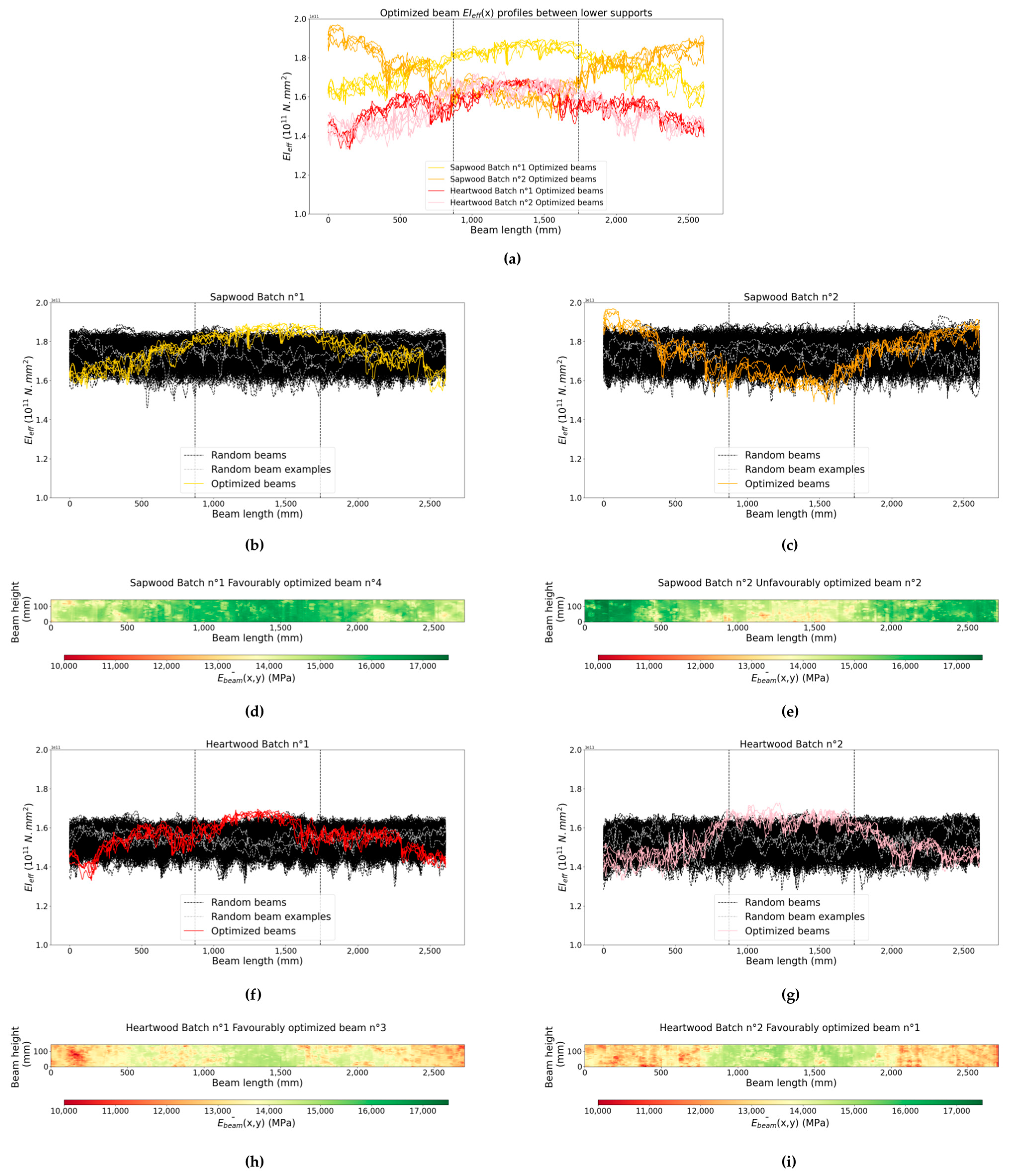
3.1. Effect of Beam Optimization on Modeled Mechanical Properties

First, observations can be made on the impact of the controlled distribution of veneers based on their quality within the different panels on their effective bending stiffness.

The colored $E{I}_{eff}\left(x\right)$ curves presented in Figure 6a are the bending stiffness profiles for each modeled and manufactured beam. They allow for a very explicit observation of the effects of the veneer positioning processes. Favorably optimization led to observing maximum bending stiffness values in the central part of the beams and a regularly decreasing bending stiffness at the ends of the beams. The opposite was also observable for unfavorably optimized beams. The dotted vertical lines represent the loading points of the four-point bending test arrangement. The black curves in Figure 6b,c,f,g represent the $E{I}_{eff}\left(x\right)$ curves of beams obtained from random positioning of veneers in the panel. The 150 cases per batch simulated represent 750 beams (5 beams cut for each panel). All displayed black curves in Figure 6b,c,f,g, and showed the possible “area of performance”. This allowed showing how the optimized bending stiffness profiles provide the best possible stiffness to fit the applied bending moment, while the random arrangements had up and downs randomly all along the beams (shown by individual grey curve examples). Figure 6d,e,h,i are examples of colormaps of the local modulus of elasticity averaged over the 15 plies of LVL beam generated from different batches ($\overline{E_{beam}}\left(x,y\right),$ as defined in Part 1). Figure 6d,h,i shows a concentration of green between loading points, corresponding to higher local modulus than in the beam end areas. There was also a variation in the color range between the sapwood beams (Figure 6d,e) and heartwood ones (Figure 6h,i), explained by a density effect between the two types of wood.

For cases of favorably optimized beams, an $E{I}_{eff}\left(x\right)$ profile was observed, with higher local values at the center of the beams than at their extremities, which corresponded well to a positioning of the veneers with lower quality at the ends and those of higher quality at the center (Figure 6b,f,g). On the contrary, for unfavorably optimized beams, a concentration of local high $E{I}_{eff}\left(x\right)$ values at extremities and lower-quality veneers at the center was observed in Figure 6c.

Comparing heartwood and sapwood, a general gap between profiles was observable on the optimized profiles. This difference was mostly imputable to a difference in the veneers’ density. To estimate this difference, an overall average of all the points in the profiles of all the sapwood and heartwood beams was performed. The average value was 1.54.10¹¹ N mm² for heartwood and 1.74.10¹¹ N mm² for sapwood (difference of 13.0%).

There was a difference between the positioning of veneers leading to the favorably optimized heartwood curves in Figure 6f,g. For the first one, there was a high local maximum between loading points (slightly above the “area of performance”), but also a low local minimum between loading points compared to the curves of the second batch. This was due to the placement algorithm, modified between the creation of the two batches to improve strength. In the first case, the requirement to place the higher-quality veneers in the center was preponderant, while in the second case, the effect of maximizing the plateau value between the loading points was sought.

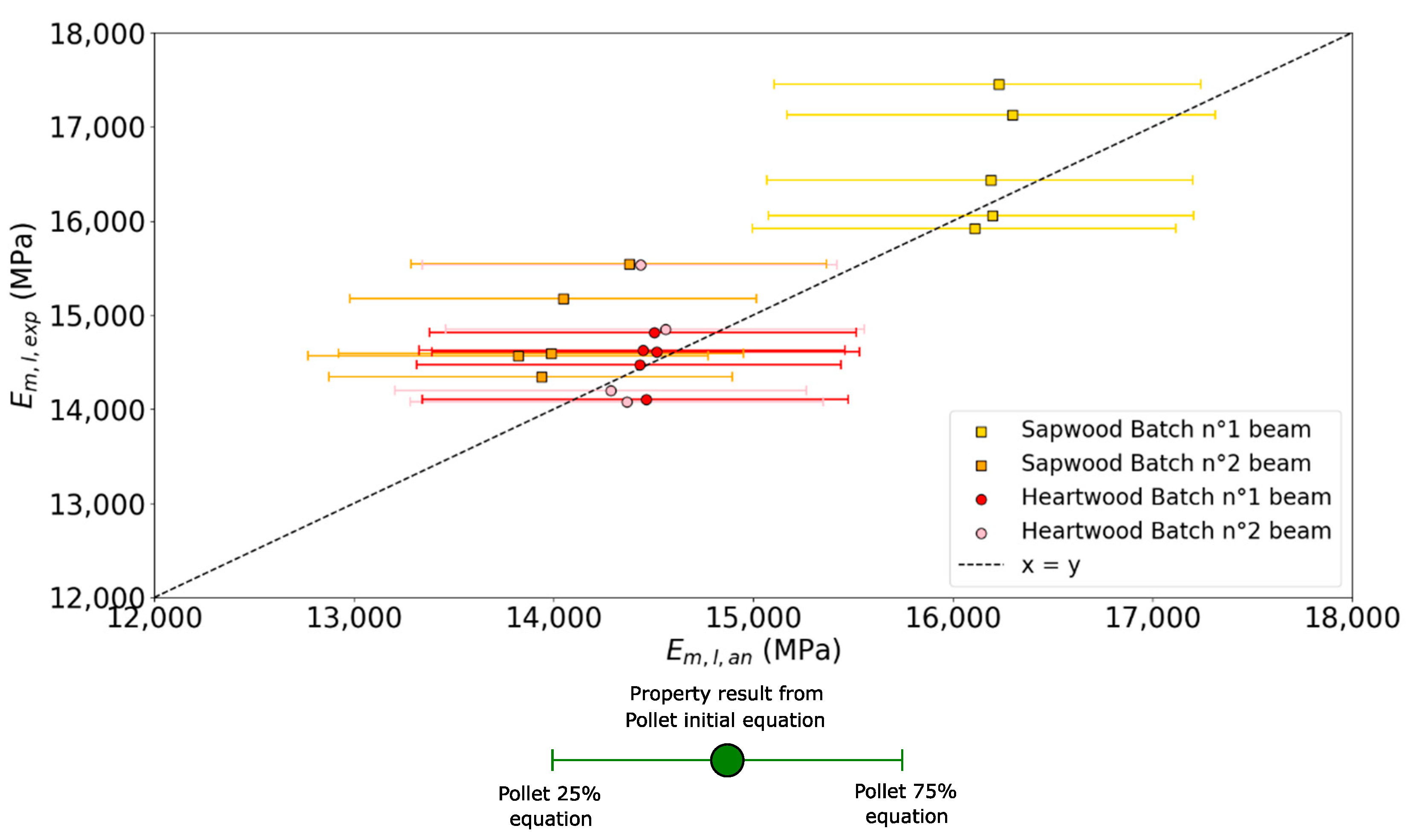
3.2. Modeling Result Analysis by Comparison with Destructive Results

To analyze the accuracy of the mechanical properties modeling of beams, a comparison was made between the results of destructive testing on the optimized beams and analytical tests on their numerical equivalent.

$E_{m,l,ex}$ experimental results were recalculated to 12% MC according to EN 384 standard, to be compared with $E_{m,l,an}$. These results are visible in Figure 7. Whisker plots enabled us to observe the domain of mechanical properties, whose edges represent the value resulting from the application of the 25% and 75% variants of the Pollet equation from Table 2.

The relative differences between modelized results from Pollet [8] mature Douglas wood equation (Equation (1)) according to experimental results were on average of −0.9% for heartwood, with a minimum deviation of −7.1% and a maximum deviation of +2.5%. For sapwood, the difference was, on average, −3.8%, with a minimum deviation of −7.5% and a maximum of +1.2%. Thus, despite the fact that this equation is applicable for mature wood, the analytical bending modeling was found to have a tendency to undervalue the local modulus of elasticity, especially for sapwood, and more clearly for unfavorable optimization. Moreover, the model exhibited difficulty perceiving the singularities of the different beams from the same panel. Hence, it tended to be relatively consistent in its predictions (R² = 0.73), but the conclusions cannot be drawn any further given the reduced number of specimens.

The experimental tests showed the optimization effect of the panels on the $E_{m,l,exp}$ and $f_{m,exp}$ results of the four batches (shown in

Table 6. Experimental results.

		Heartwood Mean Value (COV %)				Sapwood Mean Value (COV %)
			Configuration	Em,l,exp (MPa)	fm,exp (MPa)		Configuration	Em,l,exp (MPa)	fm,exp (MPa)
Representative veneer batches	Batch n°1	5 beams	Favorable optimization	14,527 (1.8)	50.96 (8.2)	5 beams	Favorable optimization	16,599 (4.0)	61.47 (6.8)
	Batch n°2	4 beams	Favorable optimization	14,665 (4.6)	49.30 (11.9)	5 beams	Unfavorable optimization	14,847 (3.3)	47.99 (11.3)

).

Indeed, the average relative deviation for $E_{m,l,exp}$ between sapwood favorably and unfavorably optimized beams was +11.8% (16,599 MPa vs. 14,847 MPa), while the relative deviation between the $E_{m,l,an}$ mean value was +15.5% (16,205 MPa vs. 14,036 MPa). The relative deviation in between number 2 and number 1 batches of heartwood-favorably optimized beams $E_{m,l,exp}$ mean value was +1.0% (14,665 MPa vs. 14,527 MPa ) while the relative gap between the $E_{m,l,an}$ mean value was −0.4% (14,413 MPa vs. 14,472 MPa). The absolute values were also very close, highlighting the great calibration of analytical model parameters, as noticeable in Figure 7.

Despite unavoidable variations between beams, these average results provided some confidence in the representativeness of the modeling method, allowing for deeper exploitation of modeling results in the following section.

Regarding bending strength in sapwood batches, there was an average relative deviation of +28.1% between the favorably optimized and unfavorably optimized batches. This value is remarkable given that only the positioning of veneers according to their quality differs between the batches. Considering the small sample of beams tested, it was difficult to conclude the predictive aspect of the model by the $E_{min}$ criterion on the strength of beams tested in four-point bending, as shown in Figure 8.

However, the effect of favorable and unfavorable optimizations on the beams of the batches was noticeable, as for local modulus of elasticity. For batch n°2 sapwood unfavorably optimized beams, the $f_{m,exp}$ bending strength was between 40 MPa and 52 MPa, while for batch n°1 favorably optimized beams, it was between 55 MPa and 67 MPa. Concerning the $E_{min}$ criterion, batch n°2 optimized beams averaged 13,091 MPa while batch number 1 optimized beams averaged 15,257 MPa (+16.5%). For heartwood, the two favorably optimized batches presented similar strength between 39 MPa and 59 MPa. It seems that, even if an increasing global trend was observed, the proposed criterion was not able to differentiate precisely the observed variation of bending strength for all favorable or unfavorable LVL composition.

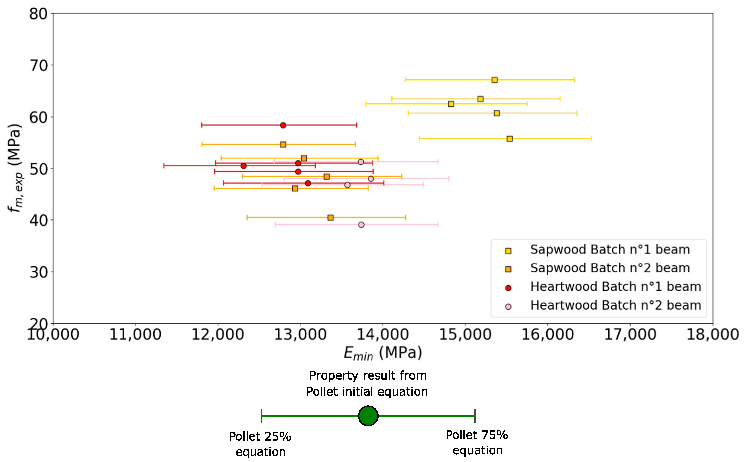
3.3. Comparison with Sorted and Unsorted Random Beams

As a point of comparison to evaluate the performance of optimized beams, random panels created using the algorithm developed in [2] were generated from the same veneer batches. Figure 9 and Figure 10 show respectively $E_{m,l,an}$ and $E_{min}$ of beams with optimized veneer placements compared to random beams made from the same veneers. Violin plots allows observing the distribution law of random values. Dots representing optimized beams enabled us to observe the optimization of the beams in relation to the random sample.

For each sample of 150 random beam results, a Shapiro–Wilk test was performed. For $E_{m,l,an}$ and $E_{min}$ random beams results, a Gaussian distribution was observed (p-value < 5%). This enables the use of 150 random beam sample trends to be relevant to conclusions in general terms. For $E_{min}$ results, the distribution was crushed over the higher values. This was due to the nature of the parameters. The local modulus elasticity was calculated for a portion of beam (5 h length). This gave a kind of averaged value. The $E_{min}$ value was by nature a minimum value for substantially the same portion of beam (6 h length).

Table 7. Summary results (12% MC).

		Heartwood					Sapwood
				Em,l,an (MPa)	Emin (MPa)				Em,l,an (MPa)	Emin (MPa)
		Amount of Panels × Amount of Beams		Mean Value (COV %)	Mean Value (COV %)	5th percentile (5th p) or Minimum Value (min)	Amount of Panels × Amount of Beams		Mean Value (COV %)	Mean Value (COV %)	5th Percentile (5th p) or Minimum Value (min)
Visual sorting (EN 635-3 standard)	Class II	150 × 5	Random positioning	13,442 (1.3)	12,542 (2.5)	12,008 (5th p)	150 × 5	Random positioning	15,319 (1.4)	14,491 (2.1)	13,962 (5th p)
	Class III-IV	150 × 5	Random positioning	13,541 (1.9)	12,328 (3.5)	11,546 (5th p)	150 × 5	Random positioning	15,122 (2.0)	13,862 (3.4)	12,958 (5th p)
Modulus of elasticity profile sorting	Class A	150 × 5	Random positioning	14,127 (1.4)	13,224 (2.5)	12,615 (5th p)	150 × 5	Random positioning	15,803 (1.2)	14,952 (2.2)	14,360 (5th p)
	Class B	150 × 5	Random positioning	12,889 (1.5)	11,800 (2.9)	11,164 (5th p)	150 × 5	Random positioning	14,599 (1.9)	13,456 (3.0)	12,675 (5th p)
Representative veneer batches	Batch n°1	1 × 5	Favourable optimization	14,472 (0.2)	12,829 (2.4)	12,313 (min)	1 × 5	Favourable optimization	16,205 (0.4)	15,257 (1.8)	14,826 (min)
		150 × 5	Random positioning	13,462 (1.6)	12,615 (2.3)	12,097 (5th p)	150 × 5	Random positioning	15,209 (1.7)	14,360 (2.3)	13,779 (5th p)
	Batch n°2	1 × 4	Favourable optimization	14,413 (0.8)	13,658 (1.3)	13,399 (min)	1 × 5	Unfavourable optimization	14,036 (1.5)	13,091 (1.9)	12,788 (min)
		150 × 5	Random positioning	13,362 (1.8)	12,466 (2.5)	11,908 (5th p)	150 × 5	Random positioning	15,254 (1.9)	14,359 (2.6)	13,712 (5th p)

summarizes the main results of the study, including Part 1 results. It compares the results of beams from optimized panels with random panels, from the same batches, and random beams of [2], made of veneers of different sorting classes. The $E_{min}$ values are presented with mean values, but also by their 5th percentile value, to continue the analogy with the strength property usually used in the construction design. In the case of the manufactured beams, since optimized batches were composed of only five beams maximum, the minimum of $E_{min}$ values was used.

First, a comment on the results of the random heartwood and sapwood batches beam test results can be made. For heartwood, there was a relative deviation of −0.7% between $\overline{E_{m,l,an}}$ of batch number 2 random beams (13,362 MPa) and batch number 1 random beams (13,462 MPa). For $\overline{E_{min}}$, the relative deviation was on average −1.2% (12,466 MPa vs. 12,615 MPa). For sapwood, relative deviations between batch number 2 and batch number 1 were quite similar for $\overline{E_{m,l,an}}$ (+0.3%, 15,254 MPa vs. 15,209 MPa) and $\overline{E_{min}}$ (14,359 MPa vs. 14,360 MPa). This allowed drawing conclusions on the correct equivalence of the veneer batches in terms of mechanical property. Concerning $E_{min}$, it was not proven that this indicator allows an accurate prediction of beam bending strength. A simple proportionality trend was shown. The results involving the $E_{min}$ were therefore indicative.

Table 7 gives information to compare results of favorable and unfavorable optimized beams quantitatively. For sapwood, the favorably optimized beams from batch number 1 had an $\overline{E_{m,l,an}}$ of 16,205 MPa and an $\overline{E_{min}}$ value of 15,257 MPa. It was respectively +15.5% and +16.6% than results of batch number 2 unfavorably optimized beams. The results of batch number 1 optimized beams could also be compared with random beams from the same batch. Thus, relative gaps of +7.6% between optimized beam $E_{min}$ minimum value and random beam $E_{min}$ 5th percentile value (13,779 MPa) were noticed. In terms of modulus of elasticity, the gap between means values was +6.5% (16,205 MPa vs. 15,209 MPa). For heartwood, the favorably optimized beams of batch number 2 had a $\overline{E_{m,l,an}}$ of 14,413 MPa and a $\overline{E_{min}}$ of 13,658 MPa. The batch number 1 heartwood favorably optimized beams had a $\overline{E_{m,l,an}}$ of 14,472 MPa and a $\overline{E_{min}}$ value of 12,829 MPa. This 6.5% difference in $\overline{E_{min}}$ is explained by the fact that, as seen in Figure 6f,g, these beams concentrated excellent local properties at the center of the beams. However, they also had a local minimum in the upper support area that was lower than batch number 2 heartwood favorably optimized beams, mainly due to the no-overlay defect function. For local modulus of elasticity, it is normal to see that this effect had very little impact (−0.4% between 14,413 MPa and 14,472 MPa) compared to the random beams generated from the same veneers.

On the basis of this better homogenization, batch number 2 favorably optimized beams, $E_{min}$ was +12.5% higher than batch number 2 random beams $E_{min}$ 5th percentile value (13,399 MPa vs. 11,908 MPa), while this gap was only +1.8% for heartwood batch number 1 (12,313 MPa vs. 12,097 MPa). For $\overline{E_{m,l,an}}$, theses gaps were respectively +7.9% (14,413 MPa vs. 13,362 MPa) for batch number 2 and +7.5% (14,472 MPa vs. 13,462 MPa) for batch number 1.

As expected, results of the random beams of the four batches of veneer, whether for $E_{min}$ or $E_{m,l,an}$, were always included between Class A and Class B. For example, batch number 1 heartwood random beams $\overline{E_{m,l,an}}$ (13,462 MPa) was between 12,889 MPa of Class B and 14,127 MPa of Class A.

It was also possible to compare the results of optimized beams composed of the veneers representative of the resource with the random beams composed of the strength classes created in [2], i.e., compare the proposed optimized use of the veneer material to the more classical strength. It can be noted that sapwood favorably optimized beams were stiffer in terms of $\overline{E_{m,l,an}}$ than all the random beam classes, and more especially than Class A (+2.5% between 16,205 MPa vs. 15,803 MPa). The same trend was true for $E_{min}$ (a minimum value of 14,826 MPa vs. a 5th percentile value of 14,360 MPa). Similarly, heartwood batch number 2 was superior to all classes ($\overline{E_{m,l,an}}$, 14,413 MPa vs. 14,127 MPa for Class A, $E_{min}$ minimum value of 13,399 MPa vs. $E_{min}$ 5th percentile value of 12,615 MPa for Class A). For heartwood batch number 1, it is true for $\overline{E_{m,l,an}}$ (14,472 MPa vs. 14,127 MPa), but $E_{min}$ minimum value was slightly lower than Class A $E_{min}$ 5th percentile value (12,313 MPa vs. 12,615 MPa). This contributes to show the beneficial effect of avoiding superposition defects, which permitted a better distribution of the defects in the zone between supports and thus improved the $E_{min}$ value in heartwood batch number 2 over heartwood batch number 1. Generally, these results prove that the proposed optimization can allow obtaining better bending stiffness from the full heterogeneous resource of peeled veneers than with a high-quality classical sorting and random LVL composing.

4. Discussion

To the best of authors’ knowledge, this study is the first to deal with the optimization of the LVL material by the consideration and exploitation of a highly heterogeneous species, not by the arrangement of the different qualities through the plies, but along the length of the material, according to an edgewise bending testing configuration. This was possible thanks to a new approach based on a numerical model fed with veneer density and local fiber angle in the veneer plan. This last parameter was measured using a new apparatus specifically designed to measure online local veneer fiber orientation.

The effects of the customized were highlighted by favorable or unfavorable optimization and were observed in the analytical and experimental results of the beams of both batches. For tests on the sapwood LVL beams, variations of +11.8% for experimental local modulus of elasticity and +28.1% for bending strength were found on average for favorably optimized batch compared to unfavorable batch.

The results presented in terms of local modulus of elasticity calculation from modelized beams were satisfactory, which means that the prediction of local properties and the analytical calculation are relatively reliable, despite sources of inaccuracies. In terms of pure modeling, the use of veneer global density, neglecting the localized effects of latewood and earlywood, is an important perspective of improvement.

The gain of the favorably optimized beams over random beams was quantifiable thanks to the analytical results, and it was more than 7.5% in terms of stiffness. However, the manufactured beams of this study had a relatively low span. The effectiveness of this method, which consists of coinciding the veneer quality with the curve of the bending moment, remains to be tested in cases of larger beams. Moreover, this method takes advantage of the variability of the veneer resource used by positioning low-quality veneer to low-stressed beam area, and conversely, thus the main advantage is to allow more efficient usage of low-quality resources.

Concerning the use of the nonsuperposition option for heartwood batch number 2, the homogenization effect was not noticeable in experimental results compared to batch number 1. Indeed, in terms of elastic mechanical property, the local modulus averaged the behavior between the loading points of the beam and did not allow for a precise conclusion to be drawn on a phenomenon evolving along this portion. Second, the number of beams was not sufficient to identify trends.

Finally, the modeling of LVL beam strength is a very complex issue. The use of $E_{min}$ as a bending strength indicator did not show very high reliability. It did, however, make it possible to distinguish, on average, the differences in performance between the batches. It was calculated with a very large number of simplifying hypotheses, intrinsically linked to analytical modeling. For example, the conditions and quality of gluing were not taken into account at all. The need to determine an indicator based on other criteria, such as local defect density or average knot spacing, remains.

References

1. NF EN 635-3. Plywood. Classification by Surface Appearance. Part 3: Softwood. 1 July 1995. Available online: https://sagaweb-afnor-org.rp1.ensam.eu/fr-FR/sw/consultation/notice/1244973?recordfromsearch=True (accessed on 29 October 2020).
2. Duriot, R.; Pot, G.; Girardon, S.; Roux, B.; Marcon, B.; Viguier, J.; Denaud, L. New Perspectives for LVL Manufacturing from Wood of Heterogeneous Quality—Part. 1: Veneer Mechanical Grading Based on Online Local Wood Fiber Orientation Measurement. Forests 2021, 12, 1264. [Google Scholar] [CrossRef]
3. Burdurlu, E.; Kilic, M.; İlçe, A.; Uzunkavak, O. The effects of ply organization and loading direction on bending strength and modulus of elasticity in laminated veneer lumber (LVL) obtained from beech (Fagus orientalis L.) and lombardy poplar (Populus nigra L.). Constr. Build. Mater. 2007, 21, 1720–1725. [Google Scholar] [CrossRef]
4. Chen, F.; Deng, J.; Li, X.; Wang, G.; Smith, L.M.; Shi, S.Q. Effect of laminated structure design on the mechanical properties of bamboo-wood hybrid laminated veneer lumber. Eur. J. Wood Prod. 2017, 75, 439–448. [Google Scholar] [CrossRef]
5. Chin, K.L.; Tahir, P.M.; H’ng, P.S. Bending Properties of Laminated Veneer Lumber Produced from Keruing (Dipterocarpus sp.) Reinforced with Low Density Wood Species. Asian J. Sci. Res. 2010, 3, 118–125. [Google Scholar] [CrossRef] [Green Version]
6. NF EN 14374. Structures en bois—LVL (Lamibois)—Exigences. Available online: https://www-batipedia-com.rp1.ensam.eu/pdf/document/QTH.pdf#zoom=100 (accessed on 25 March 2020).
7. NF EN 408+A1. Timber Structures—Structural Timber and Glued Laminated Timber—Determination of Some Physical and Mechanical Properties. 1 September 2012. Available online: https://sagaweb-afnor-org.rp1.ensam.eu/fr-FR/sw/consultation/notice/1401191?recordfromsearch=True (accessed on 29 October 2020).
8. Pollet, C.; Henin, J.-M.; Hébert, J.; Jourez, B. Effect of growth rate on the physical and mechanical properties of Douglas-fir in western Europe. Can. J. For. Res. 2017, 47, 1056–1065. [Google Scholar] [CrossRef]
9. Tropix 7. Les principales caractéristiques technologiques de 245 essences forestières tropicales—Douglas. 2012. Available online: https://tropix.cirad.fr/FichiersComplementaires/FR/Temperees/DOUGLAS.pdf (accessed on 29 October 2020).
10. NF-EN-322. Panneaux à base de bois—Determination de l’humidité. 1 June 1993. Available online: https://cobaz-afnor-org.rp1.ensam.eu/notice/norme/nf-en-322/FA020887?rechercheID=1757547&searchIndex=1&activeTab=all#id_lang_1_descripteur (accessed on 8 June 2021).
11. NF EN 384+A1. Structural Timber—Determination of Characteristic Values of Mechanical Properties and Density. 21 November 2018. Available online: https://sagaweb-afnor-org.rp1.ensam.eu/fr-FR/sw/consultation/notice/1539784?recordfromsearch=True (accessed on 29 October 2020).
12. Woodtec Fankhauser GmbH. Vacuum Press. Available online: https://www.woodtec.ch/wp-content/uploads/2020/11/Documentation-Vacuum-Press.pdf (accessed on 31 March 2021).
13. Viguier, J.; Bourgeay, C.; Rohumaa, A.; Pot, G.; Denaud, L. An innovative method based on grain angle measurement to sort veneer and predict mechanical properties of beech laminated veneer lumber. Constr. Build. Mater. 2018, 181, 146–155. [Google Scholar] [CrossRef]
14. Olsson, A.; Oscarsson, J.; Serrano, E.; Källsner, B.; Johansson, M.; Enquist, B. Prediction of timber bending strength and in-member cross-sectional stiffness variation on the basis of local wood fibre orientation. Eur. J. Wood Wood Prod. 2013, 71, 319–333. [Google Scholar] [CrossRef] [Green Version]
15. Viguier, J.; Bourreau, D.; Bocquet, J.-F.; Pot, G.; Bléron, L.; Lanvin, J.-D. Modelling mechanical properties of spruce and Douglas fir timber by means of X-ray and grain angle measurements for strength grading purpose. Eur. J. Wood Wood Prod. 2017, 75, 527–541. [Google Scholar] [CrossRef] [Green Version]
Figure 1. Linear regressions from the relationship between density and longitudinal modulus of elasticity for mature Douglas-fir clear specimens from Pollet [8].
Forests 12 01275 g001
Figure 2. Favorable placement veneer algorithm flowchart.
Forests 12 01275 g002
Figure 3. Nonsuperposition principle.
Forests 12 01275 g003
Figure 4. Panel manufacturing: (a) general view, (b) glue nozzles, (c) veneer positioning of plies, (d) pressing.
Forests 12 01275 g004
Figure 5. Four-point bending test arrangement.
Forests 12 01275 g005
Figure 6. Beam E I e f f profiles: (a) optimized beams from the four batches, (b) batch n°1 sapwood beams among random beams, (c) batch n°2 sapwood beams among random beams, (f) batch n°1 heartwood beams among random beams, (g) batch n°2 heartwood beams among random beams. Beam E b e a m ¯ ( x , y ) grid: (d) batch n°1 sapwood beam, (e) batch n°2 sapwood beam, (h) batch n°1 heartwood beam, (i) batch n°2 heartwood beam.
Forests 12 01275 g006
Figure 7. Scatter plot between analytical and experimental local modulus of elasticity.
Forests 12 01275 g007
Figure 8. Scatter plot between Emini between loading points from modelization and experimental bending strength.
Forests 12 01275 g008
Figure 9. Local elastic modulus in bending results according to cases: (a) heartwood batches, (b) sapwood batches.
Forests 12 01275 g009
Figure 10. Emini between loading points according to cases: (a) heartwood batches, (b) sapwood batches.
Forests 12 01275 g010