Article

Coupling Photosynthetic Measurements with Biometric Data to Estimate Gross Primary Productivity (GPP) in Mediterranean Pine Forests of Different Post-Fire Age

by
Christodoulos I. Sazeides
*,
Anastasia Christopoulou
and
Nikolaos M. Fyllas
Biodiversity Conservation Laboratory, Department of Environment, University of the Aegean, 81100 Mytilene, Greece
*
Author to whom correspondence should be addressed.
Forests 2021, 12(9), 1256; https://doi.org/10.3390/f12091256
Submission received: 11 July 2021 / Revised: 10 September 2021 / Accepted: 12 September 2021 / Published: 16 September 2021
(This article belongs to the Section Forest Inventory, Modeling and Remote Sensing)

Abstract

:
Quantification of forest Gross Primary Productivity (GPP) is important for understanding ecosystem function and designing appropriate carbon mitigation strategies. Coupling forest biometric data with canopy photosynthesis models can provide a means to simulate GPP across different stand ages. In this study we developed a simple framework to integrate biometric and leaf gas-exchange measurements, and to estimate GPP across four Mediterranean pine forests of different post-fire age. We used three different methods to estimate the Leaf Area Index (LAI) of the stands, and monthly gas exchange data to calibrate the photosynthetic light response of the leaves. Upscaling of carbon sequestration at the canopy level was made by implementing a Big Leaf and a Sun/Shade model, using both average and variant (monthly) photosynthetic capacity values. The Big Leaf model simulations systematically underestimated GPP compared to the Sun/Shade model simulations. Our simulations suggest an increasing GPP with age up to a stand maturity stage. The shape of the GPP trend with stand age was not affected by the method used to parameterise the model. At the scale of our study, variability in stand and canopy structure among the study sites seems to be the key determinant of GPP.

1. Introduction

Forest ecosystems are vital for the survival of human kind as they provide material, economical and recreational resources [1], as well as fresh water, soil protection and other ecosystem services [2]. Currently many scholars focus on the role of carbon (C) cycling within forests, and the way this process is affected by global change [3] and interacts with the climate system [4]. To understand C dynamics, estimation of the rate of C sequestration and C stock change in forest ecosystems is crucial for ecological and global change research and policy.
Estimation of ecosystem C fluxes is usually made by accounting for the different components of ecosystem productivity [5]. The terrestrial Gross Primary Productivity (GPP) is the amount of C that plants enchain through photosynthesis in the form of carbon dioxide (CO2). The annual and inter-annual GPP variation provides information about ecosystem dynamics and the rhythms of CO2 transposition from the atmosphere into the biosphere [6]. GPP is controlled by factors that directly regulate photosynthesis as well as by stand properties that indirectly regulate plant growth [7]. Abiotic factors that influence photosynthesis operate on short-term (hourly), mid-term (daily to monthly) and long-term (years) time scales. At short time scales, solar radiation [8], temperature [9] and humidity [10] fluctuations are the main factors that regulate photosynthesis. At mid-term scales, water and temperature fluctuations [11,12] are considered the key determinants of photosynthetic C accumulation, while at longer time scales nutrient availability and disturbances can have more prominent effects [13,14]. In forest ecosystems, stand density directly affects the Leaf Area Index (LAI), the amount of foliage area per unit ground area [15,16]. LAI is determined from the stand morphology and characteristics [17], and it is a major biotic factor controlling within-stand light availability [13,18], microclimate [19] and water balance [20], and thus the overall GPP of a stand [21]. At sites with infrequent disturbances, as stands mature and LAI reaches a local maximum [22], nutrient and water limitation may occur due to competition among trees, leading to reductions of stand-level GPP. However, disturbances such as wildfires and their regimes (frequency, interval and severity) play a crucial role in GPP dynamics, by resetting various ecosystem features [14]. Thus, a sound understanding of how abiotic factors, such as solar radiation, temperature and precipitation, and biotic factors, such as stand and canopy structure, control GPP is important to understand how forest ecosystems function on seasonal and interannual timescales.
Climate change is expected to affect the dynamics of Mediterranean forests [23]. Projected temperature increases [24,25], the uncertain distribution of water availability [26,27] and the interplay between drought and wildfire [28,29] are some of the most important agents that could shift the rate of C assimilation in Mediterranean forests. In areas surrounding the Mediterranean basin, mean annual temperature is expected to increase by up to 3–4 °C and precipitation to decrease by 20%, leading to shifts in the forest fires regime [30]. As a result, fires could disturb the consistency of forest ecosystems, creating areas with different stages of succession and species synthesis [31]. Typically, in the post-fire period, the trajectory of ecosystem productivity follows a single peak curve with the maximum of productivity achieved at middle age stands [7,32]. Following such scenarios, it is important to accurately simulate C fluxes to elucidate the role of Mediterranean forests in the global C cycle and to develop effective reforestation strategies for C sequestration.
Estimation of the C exchange from forest ecosystems is challenging due to the complex relationships between biotic and abiotic factors [33]. Currently, two methodologies are implemented to infer forest productivity, the “top–down” and the “bottom–up” approaches [33,34]. The “top–down” or meteorological approach attains the estimation using eddy-covariance flux towers [35]. This method is based on the continuous measurement of CO2 fluxes between ecosystems and the atmosphere, without segregating and quantifying the fluxes within the different C reservoirs of the ecosystem, for example the living biomass, the dead biomass and the soil biomass [36]. Although this method gives accurate estimations of net ecosystem productivity (NEP), i.e., the amount of C fixed by GPP after removing losses from autotrophic and heterotrophic respiration, it does so without the information of the components’ contribution. Therefore the estimation of GPP from eddy-flux data is made under a set of assumptions regarding the autotrophic and heterotrophic respiration rates [6,35]. Moreover, in cases that eddy-covariance flux towers operate in complex terrains and vegetation sites, additional approaches and data, such as mesoscale modelling, remote sensing and/or ecophysiological measurements, are used to accurately partition C fluxes [37].
The “bottom–up” or ecological approach consists in using finer spatial scale data, including biometric measurements, such as foliage, branch, stem and root growth and litter and root turnover rates, as well as gas exchanges measurements (photosynthesis and respiration) to understand C fluxes within an ecosystem [34,38]. Biometric data can additionally provide information about the structure and the properties of the canopy and the stand. Detailed biometric data can be used to estimate Net Primary Productivity (NPP), i.e., the amount of C fixed by GPP after excluding autotrophic respiration [39]. Such data can also be integrated with photosynthetic and respiration measurements, to ultimately infer GPP and NEP [40]. In this perspective the ecological approach is more complex but does provide the means for upscaling from the leaf to the ecosystem scale [36,41]. In contrast with the “top–down” approach, “bottom–up” studies necessitate the frequent physical presence of the researcher in the field and the associated difficulty to deliver continuous data [42]. By combining the “top–down” and the “bottom–up” approaches, more accurate estimations of ecosystem productivity can be obtained [43], although an agreement between the two methods is generally achieved after comparing multiple years of concurrent measurements [34].
Estimation of Mediterranean forests GPP has been primarily pursued through eddy-flux measurements and modelling studies [44,45,46,47,48,49]. Based on eddy-flux measurements, estimation of GPP ranges from 2.49 to 4.60 g C m−2 day−1 [45,47,49] throughout the year. On the other hand, model simulations yield relatively lower GPP from 1.15 to 2.66 g C m−2 day−1 [44,46,48] for typical Mediterranean forests. The range of aboveground NPP in Mediterranean forests has been estimated through biometric studies (0.13–0.55 g C m−2 day−1) [50] while annual NEP estimates from forest inventories can reach a rate of 0.25 g C m−2 day−1 [51]. Based on inferences from litterfall data, some studies estimate the annual NPP of Mediterranean pine forests at 1.64 Mg C·ha−1·yr−1 [50]. However, to our knowledge a systematic implementation of the “bottom up” approach integrated with ecophysiological measurements has not been implemented in Mediterranean pine forests.
To understand the interplay between tree morphological and physiological processes with the biotic and abiotic conditions of the stand and ultimately quantify C fluxes, process-based forest models can be used as a framework to integrate information on different ecosystem processes [52]. In this study we integrated the “bottom–up” approach with simple canopy photosynthesis models to estimate GPP variation in Mediterranean Pine forests (Pinus brutia Ten.) across a post-fire chronosequence on Lesvos Island, Greece. The “bottom–up” approach provides an advantage for studying Pine forests productivity on Lesvos, due to the topographic complexity and the forest structural heterogeneity arising from the fire history on the island. In regions of topographic and vegetation heterogeneity the eddy covariance flux tower approach could be biased [38]. Thus, even though the “bottom–up” approach is more labour-intensive, it can provide a sound understanding of C fluxes within an ecosystem [38], especially at finer spatial scales.
The aim of the study is to explore the key factors that control GPP variation in Mediterranean Pine forests of different post-fire age. Based on forest dynamics theory we expected an increase in GPP with post-fire age, until stands reached a stage of maturity, followed by a gradual decrease in productivity with increasing stand age. We anticipated seasonal GPP variation within stands to be primarily controlled by local weather conditions and phenological variation in foliar properties. Across different stand development stages, competition for light and the ability of canopy to capture radiative energy, expressed through LAI, was expected to be the main driver of GPP. We used three different methods to quantify LAI, based on direct and optical measurements. In order to systematically quantify variation in estimated GPP related to these sources of methodological variation, we used a factorial simulation protocol, which quantified variation in GPP across different methods of LAI and photosynthetic capacity representation.

2. Materials and Methods

2.1. Study Sites

Four permanent measurement plots of different post-fire age have been established and monitored on a monthly basis since July 2019 across the Pinus brutia forest ecosystem on the island of Lesvos, Greece (Figure 1). Lesvos lies in the Northeast Aegean Sea, with a typical Mediterranean climate, characterised by long xero-thermic periods and mild wet winters. Dry season begins at mid-April and ends at early October. The average annual temperature on the island is approximately 18 °C, with the minimum monthly temperature in January at 6.8 °C and the maximum monthly temperature in mid-July at 31 °C. Mean total annual precipitation is 645 mm with most rainfall falls in December and January [53].
The four plots (Table 1) were established across a post-fire chronosequence (13 to 92 years old) on similar elevation (166 to 306 m asl) and soil parental material (Ophilithic bedrock), using regional forest wildfire and geological maps. Soil texture and depth are presented in Table A1. During plot establishment we tried to minimise effects from recent disturbances by avoiding areas with obvious grazing or fire signs. All plots have mild slope (under 10%) and are dominated by P. brutia with several woody species, such as Quercus coccifera L., Pistacia lentiscus L., Erica spp. and Cistus spp., found in the understory, rarely above 1 m high, and mainly present in the two younger plots.
To determine stand age in October 2019, we collected increment cores from at least 12 trees per site. From each tree, we extracted two cores to minimise the possible impact of reaction wood. Samples were collected at breast-high with the use of a 5 mm increment borer. After surface preparation, tree-ring width was measured to 0.01 mm using the Time Series Analysis and Presentation software (TSAP-Win) [54] and a LINTAB (Rinntech Inc. Heidelberg, Germany) measuring table. All samples were visually and statistically cross-dated using TSAP-Win to identify the possible presence of missing or false rings [55]. Samples from each site were synchronised in one single mean chronology per site, the age of which determined the mean age of each stand (Table 1). Detailed information on dendrochronological analysis is provided in ([56], ‘under review’).
Square plots of 900 m2 were deployed and each tree above 1.3 m received a unique code for the facilitation of biometric measurements. For each tree diameter at breast height (dbh—cm) and height (H—m) were measured in July 2019 and monitored on an annual basis thereafter. The status (alive, dead) of each tree has also been recorded since the start of plot monitoring period.

2.2. Gas Exchange and Functional Traits Measurements

From July 2019 to December 2020, we measured leaf-level CO2 exchange using a LICOR 6400 (LICOR Inc., Lincoln, NE, USA) infrared gas analyser, on a monthly basis, except for August 2019/2020, October 2019 and November 2020. All measurements were made on days with typical weather conditions based on previous days’ weather forecasts. We randomly selected trees within the stand and measured light response curves (Lc) for six to ten trees each month. Measurements were made for three pairs of fully developed and healthy needles, from both sunlit (four to eight Lc measurements) and shaded (two to four Lc measurements) branches. A fully sunlit or shaded branch from the selected tree was cut by climbing on the tree and/or using telescopic scissors, and immediately placed in a water bucket where it was recut prior to leaf gas-exchange measurements [57]. Only current year’s needles were selected, or needles of the year before, in cases that the current year’s needles were not fully developed, by identifying the small and clustered sterile scales that indicate the end of the previous and the beginning of the new growth unit [58]. Light response curves were made using the 6400–02B LED Light Source chamber with red and blue LEDs (665 and 470 nm, respectively). The chamber was set up at ambient conditions of humidity and temperature (provided by the L6400 external sensors), at 400 ppm CO2 concentration, by using CO2 cartridges, and systematically changing the rate of photosynthetic active radiation (PAR) between 2000, 1800, 1600, 1400, 1200, 1000, 800, 600, 400, 200, 100, 80, 60, 40, 20 and 0 μmole quanta m−2 s−1 to measure net photosynthesis (Anet (μmole m−2 s−1)). At each PAR level, three logs of Anet were taken after at least a two-minute period during which the needles were left at the specific PAR flux to reach an equilibrium. At the end of each light curve, needles were acclimated under dark conditions for five minutes and an additional reading of leaf dark respiration (Rd (μmole m−2 s−1)) was taken. All sets of Lc measurements began 30 min to 1 h after dawn and ended at least 2 h after noon. Because the area of the needles inserted in the chamber did not fully cover the chamber area, we marked the edge points and corrected our measurements for the leaf area enclosed.
Each day, the needles used in the gas-exchange measurements were transferred to the laboratory for additional leaf traits measurements. In the lab, needles were treated in wet and dark conditions. One day later we measured wet mass (LWW—g) and thickness (Lth—mm) before scanning the needles with a portable scanner (iScan 900 dpi). Leaf area (LA—mm2) of the whole needles as well the marked area of the needles enclosed in the chamber were estimated using the ImageJ image analysis software [59]. We then oven-dried the needles for 72 h at 70 °C and measured their dry weight (LDW—g). Leaf dry mass per area (LMA—g m−2) and Leaf Dry Matter Content (LDMC) were estimated using average LWW, LDW and needle area [57].

2.3. Stand Level Measurements

At the stand level we quantified the monthly litterfall and branch fall rates. Five traps were made and installed in each plot. Every trap had a square frame (0.5 m × 0.5 m) and four legs (0.3 m height) made by PVC pipes (φ 16). Legs mounted the structure 0.3 m above the ground to prevent needle sepsis during the wet season. A fiberglass window net was installed inside each frame so as to create an inner curve with a maximum depth of 0.2 m, in order to prevent wind from removing needles and needle sepsis during the wet season. Litterfall accumulated in the traps was collected monthly and then oven-dried for 48 h at 70 °C. Needles were separated from other forms of litter, such as cones, twigs, and bark specimens. The mass of the needles was recorded and divided by the total area of the litterfall traps, for estimation of litterfall mass per m2.
The LAI of each plot was estimated using three different methods. In the first approach, namely the Litterfall Method (LFM), we used data from the litterfall traps [60,61] to estimate LAI by dividing the annual sum of litterfall mass per m2 with the annual average LMA and multiplying by the average needle lifespan (1.5 years, [62], C. Sazeides observations). In the second method, namely the Hemispherical Photography Method (HPM), we divided each plot into nine subplots where we took two fisheye photographs with a Canon EOS-60D and a fisheye lens (sigma 4.5 mm circular fisheye), mounted on a tripod and placed 1 m above the forest floor. The camera was always levelled, and its top side was oriented northward. All pictures were taken under overcast conditions, early in the morning during the spring of 2020, with a fixed aperture (f = 7.9) and were slightly underexposed (2/3 f-stops) [63]. Images were analysed using the HemiView Software (HemiView version 2.1 Delta-T Devices Ltd. Burwell, UK) and an average LAI per plot was estimated. In the third approach, namely the Ceptometer Method (CMM), an average plot-level LAI was estimated by systematically measuring incoming PAR within the plot using the AccuPAR linear PAR ceptometer (Decagon Devices, Inc., Pullman, WA, USA) and comparing with measurements outside the canopy at full light conditions. CMM LAI estimation was made with measurements taken around solar noon and the leaf distribution parameter set to X = 1. In each plot, six parallel transects with 5 m distance from each other were identified, and PAR measurements were taken every 5 m, at 1 m above the forest floor, counting a total of 36 LAI values for each plot, which were averaged to estimate a mean plot-level LAI.

2.4. Environmental and Remote Sensing Data

Ambient air humidity (RH) and temperature (T) were monitored in each site using iButton Hygrochron DS1923-F5# (iButtonLink, Whitewater, WI, USA) at a 5 h time step. The iButtons were placed at 2 m height on the north-facing side of a single tree in each plot. The period covered was between July 2020 and July 2021. For each month (i) and study site the average monthly temperature (Ti) and relative humidity (RHi) and standard deviation were calculated and compared between stands (see Figure A1). There were non-significant differences at ambient conditions among the sites in the same month. As the study plots are located within a small distance from each other, variation in Ti’s and RHi’s between plots are probably attributed to topographic variation and differences in stand structure. Since Ti and RHi data only partly overlapped with the simulation period, they were only used to describe site-specific weather conditions.
Hourly data for direct normal irradiance and diffuse horizontal irradiance were downloaded from Solcast (Solcast, 2019, Global solar irradiance data and PV system power output data, URL https://solcast.com/ (accessed on 21 January 2021)), a global solar forecasting and historical solar irradiance data company. The two variables were summed up to calculate the total normal irradiance, as the maximum irradiance that canopy received. Total irradiance (Wm−2) was converted to PAR (μmole quanta m−2 s−1) by multiplying with a constant equal to 2.1479 [64]. In addition, absorbed canopy radiation (Ic) was estimated from total irradiance using a constant absorbance coefficient (a = 0.75) to account for the fraction of incoming solar radiation that is absorbed by the foliage [65].
In order to compare our simulations with an independent dataset, we extracted for each study site the global GPP from the moderate resolution (500 m) dataset of Zhang et al. [66] for the 2000–2016 period. These estimates are based on an improved light use efficiency model and are driven by satellite data from MODIS and climate data from NCEP Reanalysis II. The mean value and the standard deviation (between years) across the 17 year-long period were used as a baseline to compare with our simulated GPP.

2.5. Statistical Analysis

For each light response curve (per branch, month and plot) we first corrected the needles’ area enclosed in the chamber and then fitted the Michaelis–Menten (MM) model across the PAR range:
A n e t = A s a t P A R / ( K m + P A R ) R d  
where Asat is the light saturated net photosynthetic rate (μmole m−2 s−1), Km is the half saturation coefficient (μmole quanta m−2 s−1), and Rd is the dark respiration rate (μmole m−2 s−1). The model was fit to data from the light response curves using the Global Optimization by Differential Evolution algorithm (package DEoptim) [67] and minimising the root sum of squares [52].
To test for seasonal differences in LMA and the parameters of the MM model we used a mixed effect (package lme4) [68] model, using plot as a fixed effect and month as a random effect term, due to the fact that our interest regarding months lies in the variation among them rather than the specific effect of each level [69]. The importance of accounting for seasonal variation was tested after comparing the Akaike’s Information Criterion (AIC) of the mixed effect model with a simple linear model without the monthly random component term (ΔAIC < 2). A Wilcoxon test was used to explore for differences between the parameters of the MM model between sunlit and shaded branches. An asymptotic test (package cvequality) was used to evaluate the coefficient of variation (CV) equality among the average and variant model estimations.

2.6. Coupling Biometric and Gas Exchange Data to Simulate Stand Level GPP

To estimate the GPP in each study plot we integrated the monthly gas exchange and biometric data with two simple canopy photosynthesis models. In particular, we ran the Big Leaf [70] and the Sun/Shade [71] canopy photosynthesis models in six different setups for the site-specific abiotic and biotic condition of each study plot. The twelve different setups are summarised in Table 2.
The “Big Leaf” approach (BL) is a simple method for estimating canopy photosynthesis, without any canopy profile information required [72]. It is based on the assumption that the scaling procedure from a single leaf to the canopy is governed by a linear relationship, assuming that canopy response to environmental stimulations is the same as that of a leaf [73]. Thus, canopy is considered as a single layer, with all leaves receiving the same radiation [71]. Requirements for this model are few, in terms of field-measured parameters as well as computational cost [74]. However, the assumptions of the BL model do not take into accounts the decrease of irradiance throughout the canopy and the relative position of leaves within the canopy. De Pury and Farquhar [71] descripted the Sun/Shade model (SS) that separates the sunlit and the shaded part of canopy. The SS model estimates the fraction of canopy that is sunlit or shaded, as well as the irradiance those two parts receive, providing a more realistic estimation of canopy photosynthesis.
Below we describe the coupling of the BL and SS models with the biometric and solar radiation data of the study plots. All algorithm developments, graphs and statistical analyses were made in R [75] using the packages lubridate [76], dplyr [77], fishmethods [78], ggplot2 [79], ggpubr [80] and tidyverse [81].
For each month and in each study plot, a discrete light response curve was available, which accounted for potential acclimation of photosynthesis to environmental variation [82,83]. The monthly Lc curves were used in the varying photosynthetic capacity model setups, while a mean Lc fitted with all available data (for measurements across all months Figure A2) was used in the constant photosynthetic capacity model setups.
In all cases, hourly radiation data were used to force the models and simulate hourly Anet under the constant and varying photosynthetic capacity model setups, with Rd set to 0 during daylight hours. Simulations were made for the period between July 2019 and December 2020. The hourly time-step simulations were summarised to monthly and annual GPP estimates for model intercomparison and validation. The estimation of the annual GPP was made for the period between July 2019 to June 2020.

2.6.1. Big Leaf Model

Scaling up productivity from the leaf to the canopy level following the BL model setup was made using:
G P P = A n e t [ 1 exp ( k b   L A I ) ] / k b  
where exp is the exponential function and kb is the beam radiation extinction coefficient of the canopy:
k b = 0.5 / sin β  
and β is the solar elevation angle (in radians) and 0.5 is the ratio of projected area to surface area of a hemisphere. Hourly values of β were estimated from the astrocalc4r function (package fishmethods).

2.6.2. Sun/Shade Model

The application of the SS model required additional calculations. We initially simulated the fraction of sunlit canopy according to:
L s u n = [ 1 exp ( k b   L A I ) ] / k b  
where Lsun is the fraction of sunlit LAI.
The shade fraction of the canopy (Lsh) was estimated from the difference between LAI and Lsun, on an hourly basis. The fraction of PAR absorbed from the sunlit part of the canopy was calculated using:
I c s u n = I l b + I l d + I l b s  
The absorbed irradiance from the sunlit canopy (Icsun) was estimated as the sum of the direct beam (Ilb), diffuse irradiance (Ild) and scattered beam irradiance (Ilbs) absorption (Equations (A1)–(A3)). The total absorbed irradiance from the canopy (Ic) was calculated from:
I c = ( 1 r c b ) I l b [ 1 exp ( k b s L A I ) ] + ( 1 r c d ) I d [ 1 exp ( k d s L A I ) ]  
with the difference between Ic and Icsun representing the irradiance absorbed by the shaded part of the canopy (Icsh). Equations for calculating rcb, rcd, kds and kbs, are summarized in Table A2. Scaling up to the canopy level following the SS model setup was made using:
G P P = [ A s a t , s u n L s u n I c s u n / ( K m , s u n + L s u n I c s u n ) ] + [ A s a t , s h L s h I c s h / ( K m , s h + L s h I c s h ) ]  

3. Results

3.1. Variation in Stand Structure across the Post-Fire Chronosequence

Variation of mean diameter at breast height among the study sites (Table 3) indicated an increasing average tree size with time since fire, with a decreasing stem density after a peak in the 40 year-old stand. Overall, LAI followed an increasing trend with time since fire, peaking at the 72 year-old plot, and slightly decreasing in the 90 year-old plot. As the plots were chosen to be undisturbed after the fire event, the slightly decrease in stem density in the 90 year-old plot was due to the self-thinning process. The LFM estimated higher values for LAI compared to HPM and CMM.

3.2. Foliage Properties and Their Seasonal Variation

Outputs from the mixed effect model indicated that the average values of both LMA and the photosynthetic MM model parameters were not different between the study plots, except for higher Asat in the 13 year-old plot, suggesting the potential for using a common (average) light response curve across all study sites (Table 4). However, significant variation in the random (month) component was also identified (Table 4), suggesting that seasonal variation should be considered (monthly photosynthetic light response model setup).
Among all foliar properties studied, LMA showed the lowest seasonal variation (Figure 2A–D, Table A3). Monthly Asat variability followed the seasonal patterns of temperature and precipitation variation (Figure 2E–H) with the highest values observed in spring. Between plots the highest seasonal variation was found in the youngest and less dense plot (Table A3). For all plots, lower Asat values were observed in the summer of 2020 (Figure 2E–H), while Km covaried with Asat (Figure 2I–L). Leaf dark respiration showed the highest seasonal variation, with middle age stands having the higher CV.
The saturated net photosynthetic rate and the dark respiration were not statistically different between sunlit and shaded needles (Asat,sun = Asat,sh, Rd,sun = Rd,sh) as inferred from the Wilcoxon tests applied within and across all plots (Table A4). However, the half saturation coefficient was different between sunlit (Km,sun) and shaded needles (Km,sh). In order to simplify our model parameterisation, a correction for Km,sh was implemented by multiplying the value of Km,sun by 0.76, estimated from the ratio of Km,sh/Km,sun across all monthly estimates.

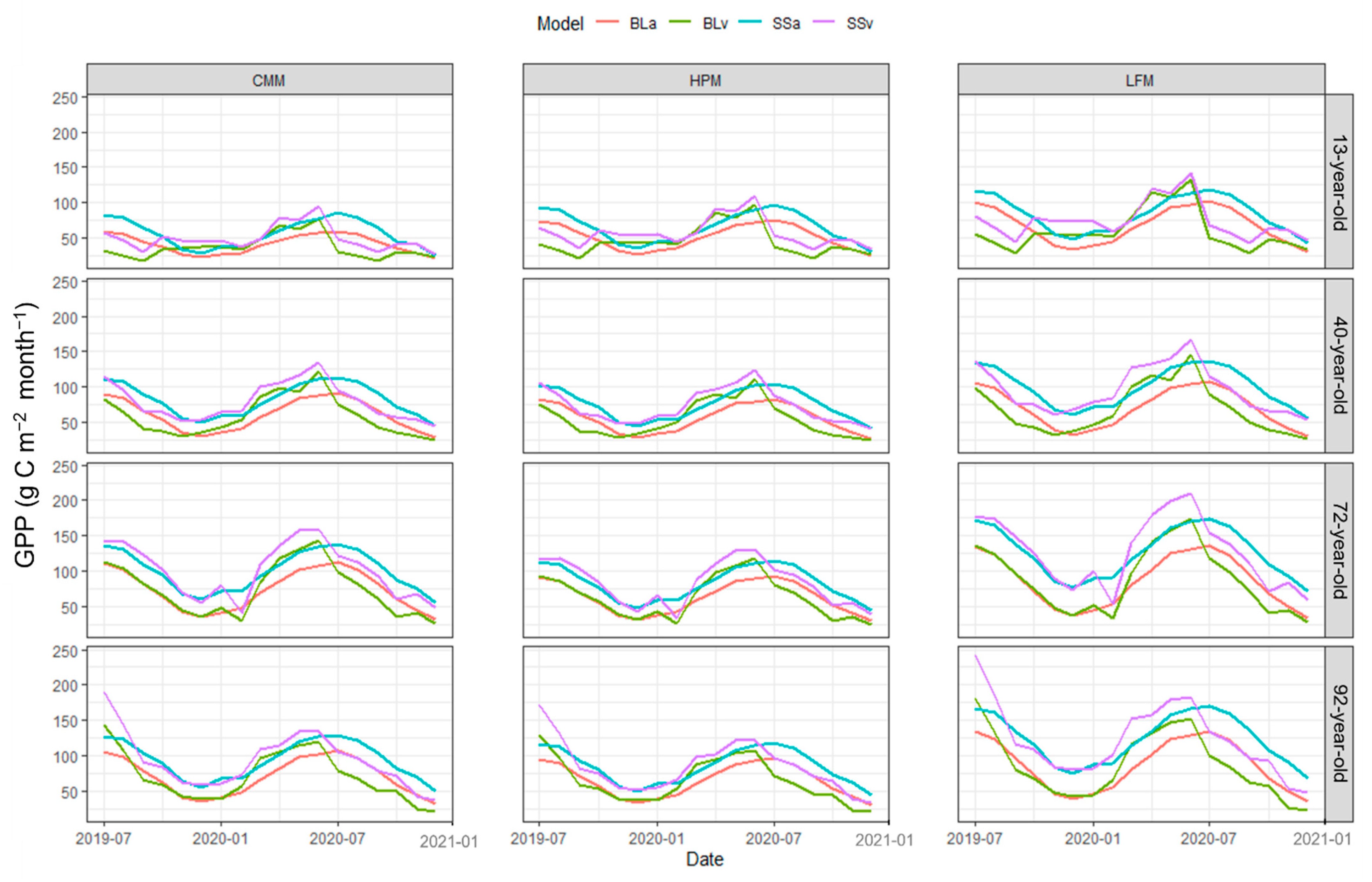
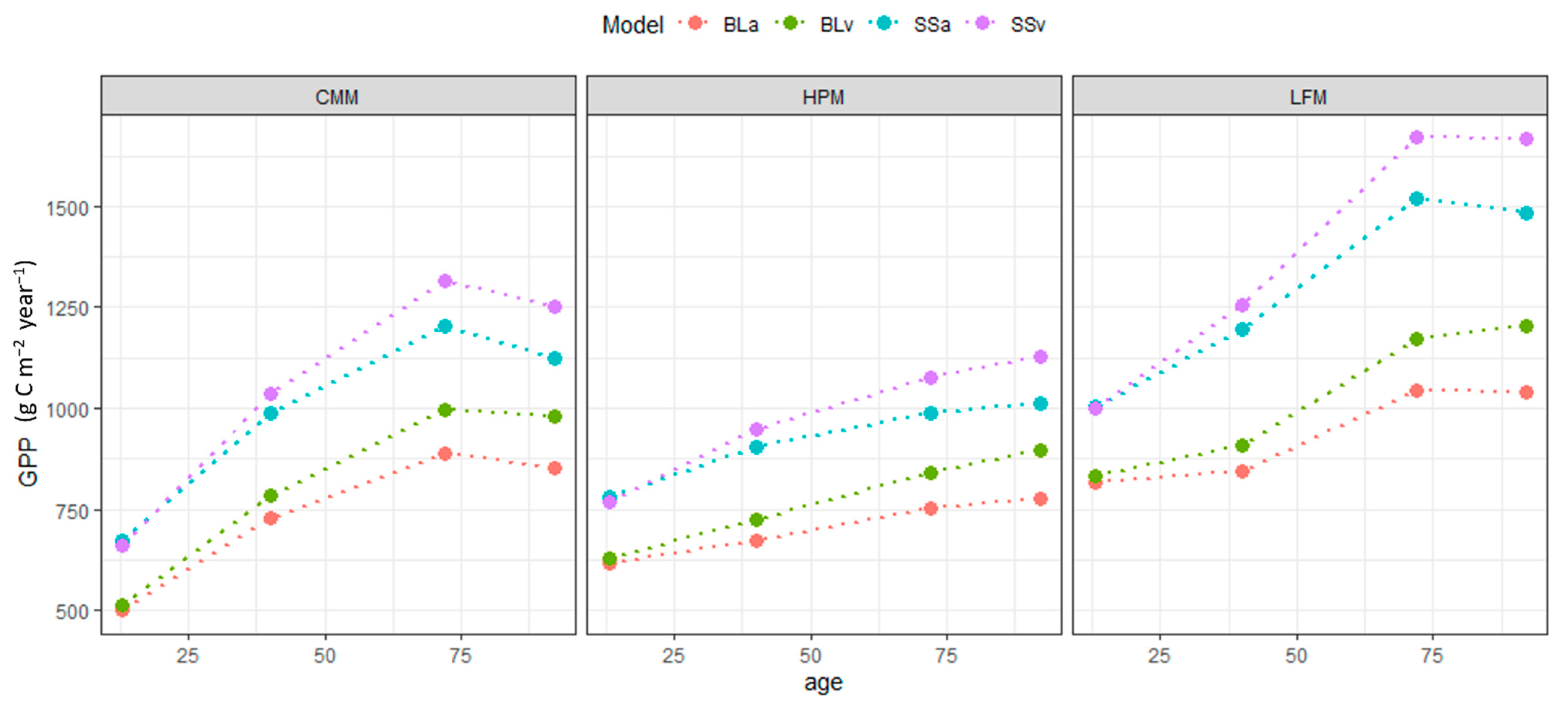
3.3. GPP Simulations

Simulated monthly GPP across the four study plots and the twelve model setups is presented in Figure 3. All model setups illustrated a characteristic peak of GPP during the growing season with the highest values in June, following seasonal variation in PAR flux and temperature. In all model setups, simulated annual GPP increased with stand age (Figure 4) until maturity (72 year-old) and then slightly decreased, except for the HPM model setups, where GPP increased continuously with post-fire time.
In general, the BL model simulated lower monthly GPP fluxes compared to the SS model, yielding a lower annual GPP across all study plots (Table 5). Compared with the independent GPP dataset predictions, the BL model estimates were within the mean ± one SD range 5 out of 24 times and the SS model estimates were within the baseline range 10 out of 24 times.
In terms of the variation related to the method used to estimate LAI, the LFM model setups yielded the highest GPP, as expected from the higher LAI input values. Under the LFM parameterisation the simulated annual GPP was 28% and 38% higher compared to the CMM and HPM methods, respectively. Compared with the independent GPP dataset predictions, the CMM model setup annual estimates were within the mean ± one SD range 4 out of 16 times, the HPM 5 out of 16 and the LFM 6 out of 16.
Models that run with the average photosynthetic capacity parameters illustrated a lower variability in simulated monthly GPP compared to the variant model setups (CVa = 42.3% vs. CVv = 52.4%, D_AD = 13.60, p < 0.001). During most of the simulation period the variant model setups simulated higher GPP than the average photosynthetic capacity models, except for the period between 07/2020 and 09/2020 (Figure 3). Compared with the independent GPP dataset predictions, the average photosynthetic capacity models were within the baseline range 7 out of 24 times, and the variant photosynthetic capacity models were so 8 out of 24 times.

4. Discussion

In this study we provided a semi-empirical framework to quantify GPP variation across Mediterranean pine forests of different post-fire age. In accordance with forest dynamics theory, we simulated an increase in GPP with stand age until a maturity stage, followed by a small decrease in older stands. The shape of the GPP curve with time did not significantly change with the method used to upscale CO2 fluxes from the leaf to the stand level. The Big Leaf model setups systematically underestimated GPP compared to the Sun/Shade model setups. Differences in the method used to parametrise our framework yielded an average plot GPP between 844 and 1166 gC m−2 y−1 across different LAI estimation methods, and an average GPP range from 934 to 1010 gC m−2 y−1 between constant and variant photosynthetic capacity setups. Overall, our simulations are within the range of GPP suggested for Mediterranean pine forests, namely from 816 to 1600 gC m−2 y−1 [48,66,84].
The trajectory of gross primary productivity with time since disturbance in unmanaged forests is frequently reported to present a parabolic shape [7] following the development of stand structure and LAI. After a wildfire, GPP immediately decreases, due to reduction in the available photosynthetic tissue biomass. Recovery of GPP can begin from the first year after the fire [85] following a steadily increasing trajectory. The degree of GPP rebound during the first few years is affected by the severity of the disturbance [14,86] as well as by water and nutrient availability [85,87]. A decade after the fire, when newly established trees take over, strong associations between GPP and canopy structure have been observed [88]. From this stage onwards, the recovery of GPP can be mostly explained by the recovery of LAI [89]. Across our post-fire chronosequence, LAI increased from younger to mature stands and then decreased at the 92 year-old stand (Table 3), probably due to competition between trees for light, water and nutrients [20,90]. Optical methods, such as CMM and HPM, generally underestimate LAI values when compared to direct and/or semi-direct methods, such as LFM, especially at forest stands [17,91]. The trend of LAI with time since the last stand-replacing fire controlled variation in GPP and shaped the typical parabolic curve with a peak in productivity at mature stands (Figure 3). This GPP trend was found in CMM and LFM model parameterisations, where stand-level LAI estimates were higher. In the HPM parameterisation, the lower LAI field estimates used to force the models yielded a continuously increasing GPP with stand age, as a result of carbon assimilation rate being away from the asymptote expected for relatively dense forest canopies with high LAI values. The results from the comparison of the variation related to the method used to estimate LAI illustrated that LAI measured using the LFM has the best agreement with the independent GPP dataset predictions. Overall, the selection of the LAI parameterisation method can have important effects on the simulation of GPP in studies that couple biometric and gas exchange data to estimate forest productivity, as has also been highlighted in satellite-data driven GPP simulation studies [92].
The control of climate, canopy structure and leaf physiology in controlling GPP has gained a lot of attention over the last decades. Many studies have explored the effect of climate [93,94], leaf traits [95,96] and canopy structure [97,98] in determining GPP across different ecosystem types. For many ecosystems, GPP increases until a peak during the growing period when solar radiation, temperature and water availability are optimum and then gradually decreases, with the contribution of the individual climate factors shifting with latitude [99,100]. This pattern has also been observed for Mediterranean forests, with GPP peaking during solar radiation and temperature optima [28,101], although for pine forest in semi-arid conditions GPP seems to maximise earlier in the year, representing a shift from radiation-controlled to moisture-controlled conditions [102]. Overall, Mediterranean forests seem to achieve a lower maximum and annual GPP, compared to tropical, subtropical and temperate forests [100]. However, the relative control of climate, canopy structure and leaf physiology on forest GPP has been studied less within similar ecosystem types (see, however, [103,104]). Among our study plots, found within relatively short distances from each other (max distance 28.2 km), similar climatic conditions prevail (Figure A1). Furthermore, no differences in the photosynthetic capacity parameters have been identified between the study sites (Table 4) and thus variability in stand and canopy structure can be considered as the main source of simulated GPP variation among the sites. Across our study sites, canopy structure variability is related to the time since the last stand-replacing fire and thus the four study plots can be used to represent the expected GPP pattern with post-fire time. In accordance with ecosystem theory, GPP seems to peak at mature stands, and thus maintenance of this forest state can be important for carbon management purposes [7].
In our simulations, seasonal variation of GPP (Figure 3) seems to be mainly driven by seasonal patterns of PAR [100]. Simulation of GPP based on satellite-driven models is frequently made through light use efficiency models [105], where primary productivity is estimated as the product of incoming PAR, the fraction of absorbed PAR and various environmental scalars (functions that do or do not limit GPP based on prevailing weather conditions and nutrient availability). These models frequently assume a constant (throughout the year) maximum efficiency of the foliage to convert the absorbed energy to carbon (like our average photosynthetic capacity models), which is being reduced by the environmental scalars [66]. Field observations suggest, however, that the photosynthetic capacity of leaves varies substantially throughout the year [84,106], as our results also show (Figure 2E–P and Table 4), and thus the use of constant photosynthetic parameter values may be inappropriate when simulating GPP [84]. In our varying photosynthetic capacity model parameterisation, we used monthly estimates of the parameters of the photosynthetic light response curve to take into account non-stomatal limitation shifts in photosynthetic capacity, such as reduced mesophyll conductance and photochemical and enzymatic limitations [107]. We further assumed that short-term effects of factors such as temperature and water availability would be less important in determining daily carbon assimilation rates, and thus avoided the use of scalars or functions that regulate canopy conductance, for example through the implementation of stomatal conductance regulation algorithms [108]. Incorporating such short-term responses of photosynthesis to weather variability would probably increase the accuracy of our simulations and reduce simulated GPP fluxes. However, in this study our purpose was to describe a simplified scheme for upscaling measurements of leaf gas-exchange to the stand level, by avoiding the use of detailed physiological algorithms, and assuming that once variation in some key foliage properties has been taken into account, patterns of incoming solar radiation might be the key determinants of forest primary productivity [52]. We however acknowledge that our simplified framework depends strongly on the availability of monthly photosynthetic data that require a significant time spent in the field.
During our study period, a strong reduction in the photosynthetic rate in July 2020 has been observed, with Asat = 5.365 (μmole m−2s−1) being 22.3% lower than the respective July 2019 Asat. Precipitation during June and July 2020 (36.7 mm) was more than three times larger than that of June and July 2019 (11 mm), suggesting that short-term effects of photosynthetic stomatal limitation might not be as important as other process such as the drought memory phenomenon [11]. In our case this would mean that in 2019, trees were adapted to dry conditions from the previous dry months, therefore creating the drought memory [109], reflecting a higher photosynthetic rate in July 2019 in contrast to July 2020, when trees did not have the pre-adaption conditions. Experiments have shown that pre-stressed plants maintain higher photosynthetic rates than non-pre-stressed plants at a drought event, even if both show similar stomatal conductance and respiration [110,111], supporting the use of seasonal shifts in photosynthetic capacity rather than regulations of stomatal conductance based on short-term weather variation.
The 13 year-old plot, which is the youngest in our plot network, illustrated the lower stand basal area and LAI. Due to small tree size the stand has not yet achieved canopy closure and is characterised by the most heterogenous microclimatic conditions. The low LAI in the 13 year-old stand results in a relatively higher percentage of tree foliage being sunlit compared to other plots (13 year-old, 56.6%, 40 year-old, 40.0%, 72 year-old, 35.9% and 92 year-old, 38.2%) [112], leading to higher Asat due to photo-acclimation. Murchie and Horton [113] supported the view that light-demanding tree species (such as P. brutia) can acclimate by changing their leaf chlorophyll content and subsequently their photosynthetic capacity. Our data revealed that photosynthetic capacity illustrated a higher seasonal variation in plots with lower LAI and canopy closure. In such stands, parts of the canopy are sunlit for longer, or if shaded, receive more radiation than denser stands. This could lead to morphological and physiological adaptation of leaves to optimise the rate of photosynthesis [114,115], as has also been found across our study sites where needles at younger stands are optimized along the LMA–photosynthetic capacity spectrum [116]. In addition, the heterogenous within-stand microclimatic conditions also probably lead to the increased variability that has been observed in gas exchange (13 year-old Asat and Km CV vs. other plots, Table A3), because of limited buffering of abiotic variability from neighbouring trees. A negative trend in Asat variability with LAI was also observed across plots, further supporting the potential effects of canopy structure-dependent photo-acclimation. Thus, the effects of canopy structure on GPP variation can be both direct (LAI amount of available photosynthetic tissue) and indirect (buffering effects on photosynthetic variability).

5. Conclusions

In this study we presented a simplified framework to estimate GPP in Mediterranean pine forests of different post-fire age. Overall, our simulations seem to be in agreement with GPP estimates from eddy-flux [84], process-based [101,117] and satellite-driven [66] models. Compared to the GPP values reported for temperate conifer forests [118], Mediterranean pine forest are probably achieving relatively lower C sequestration, due to water limitation during the dry summer period [119,120]. Mediterranean forests are currently positively contributing to the global carbon balance [121], but with the expected increase in fire frequency and severity, estimates of carbon sequestration among different stand ages are crucial to quantify their climate mitigation potential and design appropriate management strategies [118].

Author Contributions

C.I.S. and N.M.F. conceived and designed the study; C.I.S., A.C. and N.M.F. performed the field measurements; C.I.S. and N.M.F. ana-lyzed the data, A.C. contributed analysis tools; C.I.S. and N.M.F. wrote the paper. All authors have read and agreed to the published version of the manuscript.

Funding

This research is co-financed by Greece and the European Union (European Social Fund—ESF) through the Operational Programme «Human Resources Development, Education and Lifelong Learning 2014–2020» in the context of the project “Carbon fluxes across a post-fire chronosequence in Pinus brutia Ten forests” (MIS 5049513).

Institutional Review Board Statement

Not applicable.

Informed Consent Statement

Not applicable.

Data Availability Statement

Data are available upon request from the first author.

Acknowledgments

We would like to thank Christos Xagoraris for soil sample analysis, Ioannis Zevgolis for creating Figure 1, Panayiotis G. Dimitrakopoulos and Gavriil Spyroglou for their advice while setting up the plots.

Conflicts of Interest

The authors declare no conflict of interest.

Appendix A

Table A1. Soil texture and depth in each study plot.
Plot Age (years)Clay %Silt %Sand %Soil TextureSoil Depth (cm)
1362.7319.917.37clay28.3
4048.7317.9733.3clay26.6
7261.6612.8625.48clay29.2
9252.1517.3730.48clay34.8
Table A2. Data input and constants used in the Sun/Shade model.
SymbolData Source/ValueDefinition and Units
Idfrom Solcast dataDiffuse PAR per unit ground area
(μmole quanta m−2 s−1)
Ibfrom Solcast dataBeam PAR per unit ground area
(μmole quanta m−2 s−1)
rcd0.036Canopy reflection coefficient for diffuse PAR (unitless)
sc0.15Leaf scattering coefficient of PAR (unitless)
kds0.719Diffuse and scattered diffuse PAR extinction coefficient (unitless)
kbs0.46 ⁄ sin βBeam and scattered beam PAR extinction coefficient (unitless)
kb0.5 ⁄ sin β Beam radiation extinction coefficient of canopy (unitless)
rh [ 1 ( 1 s c ) ^ 0.5   ] / ( [ 1 + ( 1 s c ) ^ 0.5 ] ) Reflection coefficient of a canopy with horizontal leaves (unitless)
rcb 1 exp [ 2   r h k b / ( 1 + k b ) ] Canopy reflection coefficient for beam PAR (unitless), exp is the exponential function
Table A3. Seasonal coefficient of variation (cv) for Leaf Mass per Area (LMA, g m−2), saturated net photosynthetic rate (Asat, μmole m−2 s−1), half saturation coefficient (Km, μmole quanta m−2 s−1) and dark respiration rate (Rd, μmole m−2 s−1).
Parameter13 Year-Old40 Year-Old72 Year-Old92 Year-Old
LMA cv (%)10.813.012.510.0
Asat cv (%)49.539.831.333.2
Km cv (%)44.245.535.541.2
Rd cv (%)50.363.360.252.0
Table A4. Photosynthetic parameters of the Michaelis–Menten light response curve for sun and shade leaves in each study plot. Differences in mean values of Asat and Km were tested with a t test, with bold, (p < 0.05) indicating statistical significance. Asat saturated net photosynthetic rate (μmole m−2 s−1), Km half saturation coefficient (μmole quanta m−2 s−1) and Rd, dark respiration rate (μmole m−2 s−1).
Plot AgeLighting ConditionAsat Mean (μmole CO2 m−2 s−1)p-Value AsatKm
Mean
(μmole quanta m−2 s−1)
p-Value KmRd Mean
(μmole CO2 m−2 s−1)
p-Value RdAsatsh
/Asatsun
Kmsh
/Kmsun
Rdsun
/Rdsh
13 year-oldshade10.230.571304.440.1910.501.0000.890.701.00
13 year-oldsun11.52434.740.50
40 year-oldshade7.380.371189.330.0190.430.6220.790.591.40
40 year-oldsun9.35319.040.31
72 year-oldshade9.130.214289.340.6830.290.4610.920.920.84
72 year-oldsun9.89312.980.34
92 year-oldshade8.750.679258.810.5940.620.1290.910.840.93
92 year-oldsun9.57306.750.67
ALLshade8.600.171250.430.0070.470.3670.870.761.00
ALLsun9.87331.380.47
Equations for absorbed beam + scatter beam PAR (Equation (A1)), absorbed diffuse + scatter diffuse PAR (Equation (A2)) and absorbed scattered PAR (Equation (A3)). All units are μmole m−2 s−1. All symbols abbreviations explained at Table A2.
I l b = I b ( 1 s c ) [ 1 exp ( k b   L A I ) ]  
I l d = I d ( 1 r c d ) { 1 exp [ ( k d s + k b ) L ] }   k d s / ( k d s + k b )  
I l b s = I b     { 1 exp [ ( k bs + k b )     L A I ]   }     k b s [ ( k b s + k b ) ( 1 s c ) ] [ 1 exp ( 2   k b     L A I )   ] 2
Figure A1. Average monthly temperature (T) (upper) and relative humidity (RH) (lower panel) and standard deviation.
Forests 12 01256 g0a1
Figure A2. The composite (across all months) light response curve per plot.
Forests 12 01256 g0a2

References

  1. Pukkala, T. Which Type of Forest Management Provides Most Ecosystem Services? For. Ecosyst. 2016, 3, 9. [Google Scholar] [CrossRef] [Green Version]
  2. Rai, P.B.; Sears, R.R.; Dukpa, D.; Phuntsho, S.; Artati, Y.; Baral, H. Participatory Assessment of Ecosystem Services from Community-Managed Planted Forests in Bhutan. Forests 2020, 11, 1062. [Google Scholar] [CrossRef]
  3. Raihan, A.; Begum, R.A.; Said, M.N.M.; Abdullah, S.M.S. A Review of Emission Reduction Potential and Cost Savings through Forest Carbon Sequestration. Asian J. Water Environ. Pollut. 2019, 16, 1–7. [Google Scholar] [CrossRef]
  4. IPCC. Climate Change 2014: Mitigation of Climate Change. Working Group III Contribution to the Fifth Assessment Report of the Intergovernmental Panel on Climate Change; Cambridge University Press: Cambridge, UK; New York, NY, USA, 2014. [Google Scholar]
  5. Randerson, J.T.; Chapin, F.S.; Harden, J.W.; Neff, J.C.; Harmon, M.E. NET Ecosystem Production: A Comprehensive Measure of NET Carbon Accumulation by Ecosystems. Ecol. Appl. 2002, 12, 937–947. [Google Scholar] [CrossRef]
  6. Joiner, J.; Yoshida, Y.; Zhang, Y.; Duveiller, G.; Jung, M.; Lyapustin, A.; Wang, Y.; Tucker, C.J. Estimation of Terrestrial Global Gross Primary Production (GPP) with Satellite Data-Driven Models and Eddy Covariance Flux Data. Remote Sens. 2018, 10, 1346. [Google Scholar] [CrossRef] [Green Version]
  7. Chapin, F.S., III; Matson, P.A.; Mooney, H.A. Principles of Terrestrial Ecosystem Ecology; Springer: Berlin/Heidelberg, Germany, 2011; ISBN 0387954392. [Google Scholar]
  8. Vialet-Chabrand, S.; Matthews, J.S.A.; Simkin, A.J.; Raines, C.A.; Lawson, T. Importance of Fluctuations in Light on Plant Photosynthetic Acclimation. Plant Physiol. 2017, 173, 2163–2179. [Google Scholar] [CrossRef] [Green Version]
  9. Hüve, K.; Bichele, I.; Kaldmäe, H.; Rasulov, B.; Valladares, F.; Niinemets, Ü. Responses of Aspen Leaves to Heatflecks: Both Damaging and Non-Damaging Rapid Temperature Excursions Reduce Photosynthesis. Plants 2019, 8, 145. [Google Scholar] [CrossRef] [Green Version]
  10. Bunce, J.A. Effects of Humidity on Photosynthesis. J. Exp. Bot. 1984, 35, 1245–1251. [Google Scholar] [CrossRef]
  11. Alves, R.D.F.B.; Menezes-Silva, P.E.; Sousa, L.F.; Loram-Lourenço, L.; Silva, M.L.F.; Almeida, S.E.S.; Silva, F.G.; Perez de Souza, L.; Fernie, A.R.; Farnese, F.S. Evidence of Drought Memory in Dipteryx Alata Indicates Differential Acclimation of Plants to Savanna Conditions. Sci. Rep. 2020, 10, 16455. [Google Scholar] [CrossRef]
  12. Vico, G.; Way, D.A.; Hurry, V.; Manzoni, S. Can Leaf Net Photosynthesis Acclimate to Rising and More Variable Temperatures? Plant Cell Environ. 2019, 42, 1913–1928. [Google Scholar] [CrossRef]
  13. Yu, L.; Song, M.; Xia, Z.; Korpelainen, H.; Niinemets, Ü.; Li, C. Elevated Temperature Differently Affects Growth, Photosynthetic Capacity, Nutrient Absorption and Leaf Ultrastructure of Abies Faxoniana and Picea Purpurea under Intra- and Interspecific Competition. Tree Physiol. 2019, 39, 1342–1357. [Google Scholar] [CrossRef]
  14. Ryu, J.H.; Han, K.S.; Hong, S.; Park, N.W.; Lee, Y.W.; Cho, J. Satellite-Based Evaluation of the Post-Fire Recovery Process from the Worst Forest Fire Case in South Korea. Remote Sens. 2018, 10, 918. [Google Scholar] [CrossRef] [Green Version]
  15. Bahru, T.; Ding, Y. Effect of Stand Density, Canopy Leaf Area Index and Growth Variables on Dendrocalamus Brandisii (Munro) Kurz Litter Production at Simao District of Yunnan Province, Southwestern China. Glob. Ecol. Conserv. 2020, 23, e01051. [Google Scholar] [CrossRef]
  16. Landsberg, J.J.; Sands, P. Physiological Ecology of Forest Production: Principles, Processes and Models, 1st ed.; Academic Press: Amsterdam, The Netherlands; Boston, MA, USA, 2011; ISBN 978-0-12-810206-0. [Google Scholar]
  17. Bréda, N.J.J. Ground-Based Measurements of Leaf Area Index: A Review of Methods, Instruments and Current Controversies. J. Exp. Bot. 2003, 54, 2403–2417. [Google Scholar] [CrossRef]
  18. Binkley, D.; Campoe, O.C.; Gspaltl, M.; Forrester, D.I. Light Absorption and Use Efficiency in Forests: Why Patterns Differ for Trees and Stands. For. Ecol. Manag. 2013, 288, 5–13. [Google Scholar] [CrossRef]
  19. Hardwick, S.R.; Toumi, R.; Pfeifer, M.; Turner, E.C.; Nilus, R.; Ewers, R.M. The Relationship between Leaf Area Index and Microclimate in Tropical Forest and Oil Palm Plantation: Forest Disturbance Drives Changes in Microclimate. Agric. For. Meteorol. 2015, 201, 187–195. [Google Scholar] [CrossRef] [PubMed] [Green Version]
  20. Grier, C.G.; Running, S.W. Leaf Area of Mature Northwestern Coniferous Forests: Relation to Site Water Balance. Ecology 1977, 58, 893–899. [Google Scholar] [CrossRef] [Green Version]
  21. Asner, G.P.; Scurlock, J.M.O.; Hicke, J.A. Global Synthesis of Leaf Area Index Observations: Implications for Ecological and Remote Sensing Studies. Glob. Ecol. Biogeogr. 2003, 12, 191–205. [Google Scholar] [CrossRef] [Green Version]
  22. Luo, T.; Neilson, R.P.; Tian, H.; Vörösmarty, C.J.; Zhu, H.; Liu, S. A Model for Seasonality and Distribution of Leaf Area Index of Forests and Its Application to China. J. Veg. Sci. 2002, 13, 817–830. [Google Scholar] [CrossRef]
  23. Kouba, Y.; Camarero, J.J.; Alados, C.L. Roles of Land-Use and Climate Change on the Establishment and Regeneration Dynamics of Mediterranean Semi-Deciduous Oak Forests. For. Ecol. Manag. 2012, 274, 143–150. [Google Scholar] [CrossRef]
  24. Ozturk, T.; Ceber, Z.P.; Türkeş, M.; Kurnaz, M.L. Projections of Climate Change in the Mediterranean Basin by Using Downscaled Global Climate Model Outputs. Int. J. Climatol. 2015, 35, 4276–4292. [Google Scholar] [CrossRef]
  25. Lelieveld, J.; Hadjinicolaou, P.; Kostopoulou, E.; Giannakopoulos, C.; Pozzer, A.; Tanarhte, M.; Tyrlis, E. Model Projected Heat Extremes and Air Pollution in the Eastern Mediterranean and Middle East in the Twenty-First Century. Reg. Environ. Chang. 2014, 14, 1937–1949. [Google Scholar] [CrossRef] [Green Version]
  26. Friedlingstein, P.; Cox, P.; Betts, R.; Bopp, L.; von Bloh, W.; Brovkin, V.; Cadule, P.; Doney, S.; Eby, M.; Fung, I.; et al. Climate–Carbon Cycle Feedback Analysis: Results from the C4MIP Model Intercomparison. J. Clim. 2006, 19, 3337–3353. [Google Scholar] [CrossRef]
  27. Nolè, A.; Collalti, A.; Magnani, F.; Duce, P.; Mancino, G.; Marras, S.; Sirca, C.; Borghetti, M.; Nolè, A.; Collalti, A.; et al. Assessing Temporal Variation of Primary and Ecosystem Production in Two Mediterranean Forests Using a Modified 3-PG Model. Ann. For. Sci. 2013, 70, 729–741. [Google Scholar] [CrossRef] [Green Version]
  28. Fyllas, N.M.; Troumbis, A.Y. Simulating Vegetation Shifts in North-Eastern Mediterranean Mountain Forests under Climatic Change Scenarios. Glob. Ecol. Biogeogr. 2009, 18, 64–77. [Google Scholar] [CrossRef]
  29. Turco, M.; von Hardenberg, J.; AghaKouchak, A.; Llasat, M.C.; Provenzale, A.; Trigo, R.M. On the Key Role of Droughts in the Dynamics of Summer Fires in Mediterranean Europe. Sci. Rep. 2017, 7, 81. [Google Scholar] [CrossRef] [Green Version]
  30. FAO; Bleu Plan; Mediterranean Action Plan. State of Mediterranean Forests 2018; FAO: Rome, Italy, 2018; ISBN 9789251310472. [Google Scholar]
  31. Baeza, M.J.; Valdecantos, A.; Alloza, J.A.; Vallejo, V.R. Human Disturbance and Environmental Factors as Drivers of Long-Term Post-Fire Regeneration Patterns in Mediterranean Forests. J. Veg. Sci. 2007, 18, 243–252. [Google Scholar] [CrossRef]
  32. Bradford, J.B.; Birdsey, R.A.; Joyce, L.A.; Ryan, M.G. Tree Age, Disturbance History, and Carbon Stocks and Fluxes in Subalpine Rocky Mountain Forests: Tree Age, Disturbance, and Forest Carbon. Glob. Chang. Biol. 2008, 14, 2882–2897. [Google Scholar] [CrossRef]
  33. Kondo, M.; Ichii, K.; Takagi, H.; Sasakawa, M. Comparison of the Data-Driven Top-down and Bottom-up Global Terrestrial CO2 Exchanges: GOSAT CO2 Inversion and Empirical Eddy Flux Upscaling. J. Geophys. Res. Biogeosciences 2015, 1226–1245. [Google Scholar] [CrossRef]
  34. Gough, C.M.; Vogel, C.S.; Schmid, H.P.; Curtis, P.S. Controls on Annual Forest Carbon Storage: Lessons from the Past and Predictions for the Future. BioScience 2008, 58, 609–622. [Google Scholar] [CrossRef] [Green Version]
  35. Ouimette, A.P.; Ollinger, S.V.; Richardson, A.D.; Hollinger, D.Y.; Keenan, T.F.; Lepine, L.C.; Vadeboncoeur, M.A. Carbon Fluxes and Interannual Drivers in a Temperate Forest Ecosystem Assessed through Comparison of Top-down and Bottom-up Approache. Agric. For. Meteorol. 2018, 256, 420–430. [Google Scholar] [CrossRef] [Green Version]
  36. Malhi, Y. The Productivity, Metabolism and Carbon Cycle of Tropical Forest Vegetation. J. Ecol. 2012, 100, 65–75. [Google Scholar] [CrossRef]
  37. Baldocchi, D.D. Assessing the Eddy Covariance Technique for Evaluating Carbon Dioxide Exchange Rates of Ecosystems: Past, Present and Future. Glob. Chang. Biol. 2003, 9, 479–492. [Google Scholar] [CrossRef] [Green Version]
  38. Campioli, M.; Malhi, Y.; Vicca, S.; Luyssaert, S.; Papale, D.; Peñuelas, J.; Reichstein, M.; Migliavacca, M.; Arain, M.A.; Janssens, I.A. Evaluating the Convergence between Eddy-Covariance and Biometric Methods for Assessing Carbon Budgets of Forests. Nat. Commun. 2016, 7, 13717. [Google Scholar] [CrossRef]
  39. Clark, D.A.; Brown, S.; Kicklighter, D.W.; Chambers, J.Q.; Thomlinson, J.R.; Ni, J. Measuring Net Primary Production in Forests: Concepts and Field Methods. Ecol. Appl. 2001, 11, 356–370. [Google Scholar] [CrossRef]
  40. Malhi, Y.; Girardin, C.; Metcalfe, D.B.; Doughty, C.E.; Aragão, L.E.O.C.; Rifai, S.W.; Oliveras, I.; Shenkin, A.; Aguirre-Gutiérrez, J.; Dahlsjö, C.A.L.; et al. The Global Ecosystems Monitoring Network: Monitoring Ecosystem Productivity and Carbon Cycling across the Tropics. Biol. Conserv. 2021, 253, 108889. [Google Scholar] [CrossRef]
  41. Wang, Y.; Trudinger, C.M.; Enting, I.G. A Review of Applications of Model—Data Fusion to Studies of Terrestrial Carbon Fluxes at Different Scales. Agric. For. Meteorol. 2009, 149, 1829–1842. [Google Scholar] [CrossRef]
  42. Cheng, W.; Sims, D.A.; Luo, Y.; Coleman, J.S.; Johnson, D.W. Photosynthesis, Respiration, and Net Primary Production of Sunflower Stands in Ambient and Elevated Atmospheric CO2 Concentrations: An Invariant NPP:GPP Ratio? Glob. Chang. Biol. 2000, 6, 931–941. [Google Scholar] [CrossRef] [Green Version]
  43. Tramontana, G.; Migliavacca, M.; Jung, M.; Reichstein, M.; Keenan, T.F.; Camps-Valls, G.; Ogee, J.; Verrelst, J.; Papale, D. Partitioning Net Carbon Dioxide Fluxes into Photosynthesis and Respiration Using Neural Networks. Glob. Chang. Biol. 2020, 26, 5235–5253. [Google Scholar] [CrossRef]
  44. Sanchez-Ruiz, S.; Chiesi, M.; Fibbi, L.; Carrara, A.; Maselli, F.; Gilabert, M.A. Optimized Application of Biome-BGC for Modeling the Daily GPP of Natural Vegetation Over Peninsular Spain. J. Geophys. Res. Biogeosci. 2018, 123, 531–546. [Google Scholar] [CrossRef]
  45. Misson, L.; Rocheteau, A.; Rambal, S.; Ourcival, J.M.; Limousin, J.M.; Rodriguez, R. Functional Changes in the Control of Carbon Fluxes after 3 Years of Increased Drought in a Mediterranean Evergreen Forest? Glob. Chang. Biol. 2010, 16, 2461–2475. [Google Scholar] [CrossRef]
  46. Garbulsky, M.F.; Peñuelas, J.; Papale, D.; Filella, I. Remote Estimation of Carbon Dioxide Uptake by a Mediterranean Forest. Glob. Chang. Biol. 2008, 14, 2860–2867. [Google Scholar] [CrossRef]
  47. Maseyk, K.; Grünzweig, J.M.; Rotenberg, E.; Yakir, D. Respiration Acclimation Contributes to High Carbon-Use Efficiency in a Seasonally Dry Pine Forest. Glob. Chang. Biol. 2008, 14, 1553–1567. [Google Scholar] [CrossRef]
  48. Chiesi, M.; Maselli, F.; Bindi, M.; Fibbi, L.; Cherubini, P.; Arlotta, E.; Tirone, G.; Matteucci, G.; Seufert, G. Modelling Carbon Budget of Mediterranean Forests Using Ground and Remote Sensing Measurements. Agric. For. Meteorol. 2005, 135, 22–34. [Google Scholar] [CrossRef]
  49. Falge, E.; Baldocchi, D.D.; Tenhunen, J.; Aubinet, M.; Bakwin, P.; Berbigier, P.; Bernhofer, C.; Burba, G.; Clement, R.; Davis, K.J.; et al. Seasonality of Ecosystem Respiration and Gross Primary Production as Derived from FLUXNET Measurements. Agric. For. Meteorol. 2002, 113, 53–74. [Google Scholar] [CrossRef] [Green Version]
  50. Ogaya, R.; Peñuelas, J. Wood vs. Canopy Allocation of Aboveground Net Primary Productivity in a Mediterranean Forest during 21 Years of Experimental Rainfall Exclusion. Forests 2020, 11, 1094. [Google Scholar] [CrossRef]
  51. Murillo, J.C.R. Temporal Variations in the Carbon Budget of Forest Ecosystems in Spain. Ecol. Appl. 1997, 7, 461–469. [Google Scholar] [CrossRef]
  52. Fyllas, N.M.; Bentley, L.P.; Shenkin, A.; Asner, G.P.; Atkin, O.K.; Díaz, S.; Enquist, B.J.; Farfan-Rios, W.; Gloor, E.; Guerrieri, R.; et al. Solar Radiation and Functional Traits Explain the Decline of Forest Primary Productivity along a Tropical Elevation Gradient. Ecol. Lett. 2017, 20, 730–740. [Google Scholar] [CrossRef]
  53. Hellenic National Meteorological Service Climatic Data for Selected Stations in Greece; 2021.Hellenic National Meteorological Service Climatic Data for Selected Stations in Greece. Available online: http://emy.gr/emy/en/climatology/climatology_city?perifereia=North%20Aegean&poli=Mytilini (accessed on 16 April 2021).
  54. Rinn, F. TSAP-Time Series Analysis and Presentation for Dendrochronology and Related Applications; Version 4.64 for Microsoft Windows—User Reference; Rinntech Inc.: Heidelberg, Germany, 2011. [Google Scholar]
  55. Stokes, M.A.; Smiley, T.L. An Introduction to Tree-Ring Dating; The University of Arizona Press: Tucson, AZ, USA, 1996. [Google Scholar]
  56. Christopoulou, A.; Sazeides, C.I.; Fyllas, N.M. Patterns of tree growth and mortality in Mediterranean Brutia pine forests inferred from tree-ring analysis. Sci. Total. Environ. 2021. under review. [Google Scholar]
  57. Fyllas, N.M.; Michelaki, C.; Galanidis, A.; Evangelou, E.; Zaragoza-Castells, J.; Dimitrakopoulos, P.G.; Tsadilas, C.; Arianoutsou, M.; Lloyd, J. Functional Trait Variation Among and Within Species and Plant Functional Types in Mountainous Mediterranean Forests. Front. Plant Sci. 2020, 11, 212. [Google Scholar] [CrossRef] [Green Version]
  58. Vennetier, M.; Girard, F.; Taugourdeau, O.; Cailleret, M.; Caraglio, Y.; Sabatier, S.-A.; Ouarmim, S.; Didier, C.; Thabeet, A. Climate Change Impact on Tree Architectural Development and Leaf Area. In Climate Change—Realities, Impacts over Ice Cap, Sea Level and Risks; Singh, B.R., Ed.; InTech: Vienna, Austria, 2013; ISBN 978-953-51-0934-1. [Google Scholar]
  59. Schneider, C.A.; Rasband, W.S.; Eliceiri, K.W. NIH Image to ImageJ: 25 Years of Image Analysis. Nat. Methods 2012, 9, 671–675. [Google Scholar] [CrossRef]
  60. Petritan, I.C.; Mihăilă, V.-V.; Bragă, C.I.; Boura, M.; Vasile, D.; Petritan, A.M. Litterfall Production and Leaf Area Index in a Virgin European Beech (Fagus Sylvatica L.)—Silver Fir (Abies Alba Mill.) Forest. Dendrobiology 2020, 83, 75–84. [Google Scholar] [CrossRef]
  61. Wang, X.; Liu, F.; Wang, C. Towards a Standardized Protocol for Measuring Leaf Area Index in Deciduous Forests with Litterfall Collection. For. Ecol. Manag. 2019, 447, 87–94. [Google Scholar] [CrossRef]
  62. Frankis, M.P. Morphology and Affinities of Pinus Brutia. In Proceedings of the International Symposium on Pinus Brutia Ten, Marmaris, Turkey, 18–23 October 1993; INTECH Open Access Publisher: Rijeka, Croatia, 1993; pp. 11–18. [Google Scholar] [CrossRef] [Green Version]
  63. Fyllas, N.M.; Dimitrakopoulos, P.G.; Troumbis, A.Y. Regeneration Dynamics of a Mixed Mediterranean Pine Forest in the Absence of Fire. For. Ecol. Manag. 2008, 256, 1552–1559. [Google Scholar] [CrossRef]
  64. Papaioannou, G.; Papanikolaou, N.; Retalis, D. Relationships of Photosynthetically Active Radiation and Shortwave Irradiance. Theor. Appl. Climatol. 1993, 48, 23–27. [Google Scholar] [CrossRef]
  65. Valladares, F.; Skillman, J.B.; Pearcy, R.W. Convergence in Light Capture Efficiencies among Tropical Forest Understory Plants with Contrasting Crown Architectures: A Case of Morphological Compensation. Am. J. Bot. 2002, 89, 1275–1284. [Google Scholar] [CrossRef] [PubMed] [Green Version]
  66. Zhang, Y.; Xiao, X.; Wu, X.; Zhou, S.; Zhang, G.; Qin, Y.; Dong, J. A Global Moderate Resolution Dataset of Gross Primary Production of Vegetation for 2000–2016. Sci. Data 2017, 4, 170165. [Google Scholar] [CrossRef] [Green Version]
  67. Mullen, K.; Ardia, D.; Gil, D.; Windover, D.; Cline, J. DEoptim: An R Package for Global Optimization by Differential Evolution. J. Stat. Softw. 2011, 40, 1–26. [Google Scholar] [CrossRef] [Green Version]
  68. Bates, D.; Maechler, M.; Bolker, B.; Walker, S. Fitting Linear Mixed-Effects Models Using Lme4. arXiv 2015, arXiv:1406.5823. [Google Scholar] [CrossRef]
  69. Bolker, B.M.; Brooks, M.E.; Clark, C.J.; Geange, S.W.; Poulsen, J.R.; Stevens, M.H.H.; White, J.-S.S. Generalized Linear Mixed Models: A Practical Guide for Ecology and Evolution. Trends Ecol. Evol. 2009, 24, 127–135. [Google Scholar] [CrossRef]
  70. Hikosaka, K.; Niinemets, Ü.; Anten, N.P.R. Canopy Photosynthesis: From Basics to Applications; Springer: Dordrecht, The Netherlands, 2016; pp. 1–428. [Google Scholar]
  71. De Pury, D.G.G.; Farquhar, G.D. Simple Scaling of Photosynthesis from Leaves to Canopies without the Errors of Big-Leaf Models. Plant Cell Environ. 1997, 20, 537–557. [Google Scholar] [CrossRef]
  72. Raulier, F.; Bernier, P.Y.; Ung, C.H. Canopy Photosynthesis of Sugar Maple (Acer Saccharum): Comparing Big-Leaf and Multilayer Extrapolations of Leaf-Level Measurements. Tree Physiol. 1999, 19, 407–420. [Google Scholar] [CrossRef] [Green Version]
  73. Friend, A.D. Modelling Canopy CO2 Fluxes: Are “big-Leaf” Simplifications Justified? Glob. Ecol. Biogeogr. 2001, 10, 603–619. [Google Scholar] [CrossRef]
  74. Dai, Y.; Dickinson, R.E.; Wang, Y.P. A Two-Big-Leaf Model for Canopy Temperature, Photosynthesis, and Stomatal Conductance. J. Clim. 2004, 17, 2281–2299. [Google Scholar] [CrossRef]
  75. R Core Team. R: A Language and Environment for Statistical Computing; R Foundation for Statistical Computing: Vienna, Austria, 2013; Available online: http://www.R-project.org/ (accessed on 16 April 2021).
  76. Grolemund, G.; Wickham, H. Dates and Times Made Easy with lubridate. J. Stat. Softw. 2011, 40, 1–25. Available online: https://www.jstatsoft.org/v40/i03/ (accessed on 16 April 2021). [CrossRef]
  77. Wickham, H.; François, R.; Henry, L.; Müller, K. Dplyr: A Grammar of Data Manipulation. R Package Version 2021, 1.0.4. Available online: https://CRAN.R-project.org/package=dplyr (accessed on 16 April 2021).
  78. Nelson, A.G. Fishmethods: Fishery Science Methods and Models. R Package Version 1.11-1. 2019. Available online: https://CRAN.R-project.org/package=fishmethods (accessed on 16 April 2021).
  79. Wickham, H. Ggplot2: Elegant Graphics for Data Analysis; Springer: New York, NY, USA, 2016. [Google Scholar]
  80. Kassambara, A. Ggpubr: ‘Ggplot2’ Based Publication Ready Plots. R Package Version 0.4.0. 2020. Available online: https://CRAN.R-project.org/package=ggpubr (accessed on 16 April 2021).
  81. Wickham, H.; Averick, M.; Bryan, J.; Chang, W.; McGowan, D.L.; François, R.; Grolemund, G.; Hayes, A.; Henry, L.; Hester, J.; et al. Welcome to the tidyverse. J. Open Source Softw. 2019, 4, 1686. [Google Scholar] [CrossRef]
  82. Keenan, T.; Garcıa, R.; Friend, A.D.; Zaehle, S.; Gracia, C.; Sabate, S. Improved Understanding of Drought Controls on Seasonal Variation in Mediterranean Forest Canopy CO2 and Water FLuxes through Combined in Situ Measurements and Ecosystem Modelling. Biogeosciences 2009, 6, 1423–1444. [Google Scholar] [CrossRef] [Green Version]
  83. Sperlich, D.; Chang, C.T.; Penuelas, J.; Gracia, C.; Sabate, S. Seasonal Variability of Foliar Photosynthetic and Morphological Traits and Drought Impacts in a Mediterranean Mixed Forest. Tree Physiol. 2015, 35, 501–520. [Google Scholar] [CrossRef] [PubMed]
  84. Jarosz, N.; Brunet, Y.; Lamaud, E.; Irvine, M.; Bonnefond, J.-M.; Loustau, D. Carbon Dioxide and Energy Flux Partitioning between the Understorey and the Overstorey of a Maritime Pine Forest during a Year with Reduced Soil Water Availability. Agric. For. Meteorol. 2008, 148, 1508–1523. [Google Scholar] [CrossRef] [Green Version]
  85. Sun, Q.; Meyer, W.S.; Koerber, G.R.; Marschner, P. Rapid Recovery of Net Ecosystem Production in a Semi-Arid Woodland after a Wildfire. Agric. For. Meteorol. 2020, 291, 108099. [Google Scholar] [CrossRef]
  86. Li, X.; Zhang, H.; Yang, G.; Ding, Y.; Zhao, J. Post-Fire Vegetation Succession and Surface Energy Fluxes Derived from Remote Sensing. Remote Sens. 2018, 10, 1000. [Google Scholar] [CrossRef] [Green Version]
  87. Liu, X.; Pan, C. Effects of Recovery Time after Fire and Fire Severity on Stand Structure and Soil of Larch Forest in the Kanas National Nature Reserve, Northwest China. J. Arid Land 2019, 11, 811–823. [Google Scholar] [CrossRef] [Green Version]
  88. Bolton, D.K.; Coops, N.C.; Hermosilla, T.; Wulder, M.A.; White, J.C. Assessing Variability in Post-Fire Forest Structure along Gradients of Productivity in the Canadian Boreal Using Multi-Source Remote Sensing. J. Biogeogr. 2017, 44, 1294–1305. [Google Scholar] [CrossRef]
  89. Ueyama, M.; Iwata, H.; Nagano, H.; Tahara, N.; Iwama, C.; Harazono, Y. Carbon Dioxide Balance in Early-Successional Forests after Forest Fires in Interior Alaska. Agric. For. Meteorol. 2019, 275, 196–207. [Google Scholar] [CrossRef]
  90. Waring, R.H. Estimating Forest Growth and Efficiency in Relation to Canopy Leaf Area. In Advances in Ecological Research; Elsevier: Amsterdam, The Netherlands, 1983; Volume 13, pp. 327–354. ISBN 978-0-12-013913-2. [Google Scholar]
  91. Liu, Z.; Chen, J.M.; Jin, G.; Qi, Y. Estimating Seasonal Variations of Leaf Area Index Using Litterfall Collection and Optical Methods in Four Mixed Evergreen-Deciduous Forests. Agric. For. Meteorol. 2015, 209–210, 36–48. [Google Scholar] [CrossRef]
  92. Xie, X.; Li, A.; Jin, H.; Tan, J.; Wang, C.; Lei, G.; Zhang, Z.; Bian, J.; Nan, X. Assessment of Five Satellite-Derived LAI Datasets for GPP Estimations through Ecosystem Models. Sci. Total. Environ. 2019, 690, 1120–1130. [Google Scholar] [CrossRef]
  93. Zhang, Y.; Xu, M.; Chen, H.; Adams, J. Global Pattern of NPP to GPP Ratio Derived from MODIS Data: Effects of Ecosystem Type, Geographical Location and Climate. Glob. Ecol. Biogeogr. 2009, 18, 280–290. [Google Scholar] [CrossRef]
  94. Beer, C.; Reichstein, M.; Tomelleri, E.; Ciais, P.; Jung, M.; Carvalhais, N.; Rodenbeck, C.; Arain, M.A.; Baldocchi, D.; Bonan, G.B.; et al. Terrestrial Gross Carbon Dioxide Uptake: Global Distribution and Covariation with Climate. Science 2010, 329, 834–838. [Google Scholar] [CrossRef] [PubMed] [Green Version]
  95. Wang, Y.P.; Lu, X.J.; Wright, I.J.; Dai, Y.J.; Rayner, P.J.; Reich, P.B. Correlations among Leaf Traits Provide a Significant Constraint on the Estimate of Global Gross Primary Production: Correlations of Leaf Traits on Gpp. Geophys. Res. Lett. 2012, 39, L19405. [Google Scholar] [CrossRef]
  96. He, N.; Liu, C.; Tian, M.; Li, M.; Yang, H.; Yu, G.; Guo, D.; Smith, M.D.; Yu, Q.; Hou, J. Variation in Leaf Anatomical Traits from Tropical to Cold-temperate Forests and Linkage to Ecosystem Functions. Funct. Ecol. 2018, 32, 10–19. [Google Scholar] [CrossRef] [Green Version]
  97. Migliavacca, M.; Perez-Priego, O.; Rossini, M.; El-Madany, T.S.; Moreno, G.; van der Tol, C.; Rascher, U.; Berninger, A.; Bessenbacher, V.; Burkart, A.; et al. Plant Functional Traits and Canopy Structure Control the Relationship between Photosynthetic CO2 Uptake and Far-red Sun-induced Fluorescence in a Mediterranean Grassland under Different Nutrient Availability. New Phytol. 2017, 214, 1078–1091. [Google Scholar] [CrossRef] [Green Version]
  98. Shi, H.; Li, L.; Eamus, D.; Huete, A.; Cleverly, J.; Tian, X.; Yu, Q.; Wang, S.; Montagnani, L.; Magliulo, V.; et al. Assessing the Ability of MODIS EVI to Estimate Terrestrial Ecosystem Gross Primary Production of Multiple Land Cover Types. Ecol. Indic. 2017, 72, 153–164. [Google Scholar] [CrossRef] [Green Version]
  99. Xia, J.; Niu, S.; Ciais, P.; Janssens, I.A.; Chen, J.; Ammann, C.; Arain, A.; Blanken, P.D.; Cescatti, A.; Bonal, D.; et al. Joint Control of Terrestrial Gross Primary Productivity by Plant Phenology and Physiology. Proc. Natl. Acad. Sci. USA 2015, 112, 2788–2793. [Google Scholar] [CrossRef] [PubMed] [Green Version]
  100. Zhang, W.; Yu, G.; Chen, Z.; Zhang, L.; Wang, Q.; Zhang, Y.; He, H.; Han, L.; Chen, S.; Han, S.; et al. Attribute Parameter Characterized the Seasonal Variation of Gross Primary Productivity (AGPP): Spatiotemporal Variation and Influencing Factors. Agric. For. Meteorol. 2020, 280, 107774. [Google Scholar] [CrossRef]
  101. Allard, V.; Ourcival, J.M.; Rambal, S.; Joffre, R.; Rocheteau, A. Seasonal and Annual Variation of Carbon Exchange in an Evergreen Mediterranean Forest in Southern France: CO2 Fluxes of A Mediterranean Forest. Glob. Chang. Biol. 2008, 14, 714–725. [Google Scholar] [CrossRef]
  102. Wang, H.; Gitelson, A.; Sprintsin, M.; Rotenberg, E.; Yakir, D. Ecophysiological Adjustments of a Pine Forest to Enhance Early Spring Activity in Hot and Dry Climate. Environ. Res. Lett. 2020, 15, 114054. [Google Scholar] [CrossRef]
  103. Duursma, R.A.; Kolari, P.; Peramaki, M.; Pulkkinen, M.; Makela, A.; Nikinmaa, E.; Hari, P.; Aurela, M.; Berbigier, P.; Bernhofer, C.H.; et al. Contributions of Climate, Leaf Area Index and Leaf Physiology to Variation in Gross Primary Production of Six Coniferous Forests across Europe: A Model-Based Analysis. Tree Physiol. 2009, 29, 621–639. [Google Scholar] [CrossRef] [Green Version]
  104. Fyllas, N.M.; Christopoulou, A.; Galanidis, A.; Michelaki, C.Z.; Giannakopoulos, C.; Dimitrakopoulos, P.G.; Arianoutsou, M.; Gloor, M. Predicting Species Dominance Shifts across Elevation Gradients in Mountain Forests in Greece under a Warmer and Drier Climate. Reg. Environ. Chang. 2017, 17, 1165–1177. [Google Scholar] [CrossRef]
  105. Hilker, T.; Coops, N.C.; Wulder, M.A.; Black, T.A.; Guy, R.D. The Use of Remote Sensing in Light Use Efficiency Based Models of Gross Primary Production: A Review of Current Status and Future Requirements. Sci. Total. Environ. 2008, 404, 411–423. [Google Scholar] [CrossRef] [Green Version]
  106. Wang, Q.; Iio, A.; Tenhunen, J.; Kakubari, Y. Annual and Seasonal Variations in Photosynthetic Capacity of Fagus Crenata along an Elevation Gradient in the Naeba Mountains, Japan. Tree Physiol. 2008, 28, 277–285. [Google Scholar] [CrossRef] [Green Version]
  107. Flexas, J.; Diaz-Espejo, A.; Gago, J.; Gallé, A.; Galmés, J.; Gulías, J.; Medrano, H. Photosynthetic Limitations in Mediterranean Plants: A Review. Environ. Exp. Bot. 2014, 103, 12–23. [Google Scholar] [CrossRef]
  108. Buckley, T.N. Modeling Stomatal Conductance. Plant Physiol. 2017, 174, 572–582. [Google Scholar] [CrossRef]
  109. Backhaus, S.; Kreyling, J.; Grant, K.; Beierkuhnlein, C.; Walter, J.; Jentsch, A. Recurrent Mild Drought Events Increase Resistance Toward Extreme Drought Stress. Ecosystems 2014, 17, 1068–1081. [Google Scholar] [CrossRef]
  110. Menezes-Silva, P.E.; Sanglard, L.M.V.P.; Ávila, R.T.; Morais, L.E.; Martins, S.C.V.; Nobres, P.; Patreze, C.M.; Ferreira, M.A.; Araújo, W.L.; Fernie, A.R.; et al. Photosynthetic and Metabolic Acclimation to Repeated Drought Events Play Key Roles in Drought Tolerance in Coffee. J. Exp. Bot. 2017, 68, 4309–4322. [Google Scholar] [CrossRef]
  111. Ben Abdallah, M.; Methenni, K.; Nouairi, I.; Zarrouk, M.; Youssef, N.B. Drought Priming Improves Subsequent More Severe Drought in a Drought-Sensitive Cultivar of Olive Cv. Chétoui. Sci. Hortic. 2017, 221, 43–52. [Google Scholar] [CrossRef] [PubMed] [Green Version]
  112. Lefsky, M.A.; Cohen, W.B.; Acker, S.A.; Parker, G.G.; Spies, T.A.; Harding, D. Lidar Remote Sensing of the Canopy Structure and Biophysical Properties of Douglas-Fir Western Hemlock Forests. Remote Sens. Environ. 1999, 70, 339–361. [Google Scholar] [CrossRef]
  113. Murchie, E.H.; Horton, P. Acclimation of Photosynthesis to Irradiance and Spectral Quality in British Plant Species: Chlorophyll Content, Photosynthetic Capacity and Habitat Preference. Plant Cell Environ. 1997, 20, 438–448. [Google Scholar] [CrossRef]
  114. Yin, Z.H.; Johnson, G.N. Photosynthetic Acclimation of Higher Plants to Growth in Fluctuating Light Environments. Photosynth. Res. 2000, 63, 97–107. [Google Scholar] [CrossRef]
  115. Walters, R.G.; Horton, P. Acclimation of Arabidopsis Thaliana to the Light Environment: Changes in Composition of the Photosynthetic Apparatus. Planta 1994, 195. [Google Scholar] [CrossRef]
  116. Sazeides, C.I.; Fyllas, N.M.; Christopoulou, A. Seasonal Variation in Foliar Properties in Mediterranean Pine Forests of Different Post-Fire Age. In EGU General Assembly Conference Abstracts; EGU: Munich, Germany, 2021; p. EGU21-1064. [Google Scholar]
  117. Chiesi, M.; Fibbi, L.; Genesio, L.; Gioli, B.; Magno, R.; Maselli, F.; Moriondo, M.; Vaccari, F.P. Integration of Ground and Satellite Data to Model Mediterranean Forest Processes. Int. J. Appl. Earth Obs. Geoinf. 2011, 13, 504–515. [Google Scholar] [CrossRef]
  118. Anderson-Teixeira, K.J.; Herrmann, V.; Banbury Morgan, R.; Bond-Lamberty, B.; Cook-Patton, S.C.; Ferson, A.E.; Muller-Landau, H.C.; Wang, M.M.H. Carbon Cycling in Mature and Regrowth Forests Globally. Environ. Res. Lett. 2021, 16, 053009. [Google Scholar] [CrossRef]
  119. Rambal, S.; Ourcival, J.-M.; Joffre, R.; Mouillot, F.; Nouvellon, Y.; Reichstein, M.; Rocheteau, A. Drought Controls over Conductance and Assimilation of a Mediterranean Evergreen Ecosystem: Scaling from Leaf to Canopy: SCALING DROUGHT FROM LEAF TO CANOPY. Glob. Chang. Biol. 2003, 9, 1813–1824. [Google Scholar] [CrossRef]
  120. Liu, J.; Rambal, S.; Mouillot, F. Soil Drought Anomalies in MODIS GPP of a Mediterranean Broadleaved Evergreen Forest. Remote Sens. 2015, 7, 1154–1180. [Google Scholar] [CrossRef] [Green Version]
  121. Harris, N.L.; Gibbs, D.A.; Baccini, A.; Birdsey, R.A.; de Bruin, S.; Farina, M.; Fatoyinbo, L.; Hansen, M.C.; Herold, M.; Houghton, R.A.; et al. Global Maps of Twenty-First Century Forest Carbon Fluxes. Nat. Clim. Chang. 2021, 11, 234–240. [Google Scholar] [CrossRef]
Figure 1. Distribution of the four study plots across the island of Lesvos. AMAL is the 13 year-old plot, PEV is the 40 year-old plot, LML is the 72 year-old plot and ACHL is the 92 year-old plot.
Forests 12 01256 g001
Figure 2. Seasonal variation of Leaf Mass per Area (LMA, (AD)), saturated net photosynthetic rate (Asat, (EH)), half saturation coefficient (Km, (IL)) and dark respiration rate (Rd, (MP)) across all study plots. Curves are locally weighted scatterplot smoothing regression analyses with a 95% confidence interval (shaded area) and dots are the individual measurements.
Forests 12 01256 g002
Figure 3. Gross Primary Productivity (GPP) monthly estimations for the examined period by the Big Leaf model with average Asat and Km, (BLa)—red line, Big Leaf with variation of Asat and Km (BLv)—green line, Sun/Shade model with average Asat and Km, (SSa)—blue line, and Sun/Shade model with variation of Asat and Km, (SSv)—purple line for all three methods of LAI estimation, ceptometer method (CMM), hemispherical photography method (HPM) and litterfall method (LFM).
Forests 12 01256 g003
Figure 4. Annual GPP estimation with time since last stand-replacing fire based on different model setups. Big Leaf model with average Asat and Km, (BLa)—red line, Big Leaf with variation of Asat and Km (BLv)—green line, Sun/Shade model with average Asat and Km, (SSa)—blue line, and Sun/Shade model with variation of Asat and Km (SSv)—purple line for all three methods of LAI estimation, ceptometer method (CMM), hemispherical photography method (HPM) and litterfall method (LFM). Big dots represent plot-specific simulations, and dotted lines represent a generic trend with age.
Forests 12 01256 g004
Table 1. Characteristics of the study plots. AMAL is the 13 year-old plot, PEV is the 40 year-old plot, LML is the 72 year-old plot and ACHL is the 92 year-old plot.
PlotLat 1Lon 1Stand Age (y)Inclination %Orientation
AMAL39.0226.591310SE
PEV39.1626.37405SW
LML39.1626.387210SW
ACHL39.1326.30920-
1 Coordinates are given in decimal degrees.
Table 2. Overview of the six different model setups. See Equation (1) for description of the light response model parameters. Leaf Area Index (LAI) estimated using the following: Hemispherical Photography method (HPM), Litterfall method (LFM) and Ceptometer Method (CMM).
ModelPhotosynthetic Capacity SetupsLAI Setups
Big Leaf (BL)
Model
Monthly (variant) photosynthetic light response parameters HPM
LFM
CMM
Annual (average) photosynthetic light response parametersHPM
LFM
CMM
Sun/Shade (SS)
Model
Monthly (variant) photosynthetic light response parametersHPM
LFM
CMM
Annual (average) photosynthetic lightHPM
LFM
CMM
Table 3. Variation in stand structure across the study plots. Leaf Area Index (LAI) was estimated with three different methods (see text for details). Diameter at breast height (dbh) measured for trees with a diameter > 1 cm. Hemispherical Photography method (HPM), Litterfall method (LFM) and Ceptometer Method (CMM).
Stand Age
(Years)
Mean Tree Height (m)Trees/Plot (no/900 m2)Mean dbh (cm)Basal Area
(m2 ha−1)
LAI Method
HPMLFMCMM
131.93991.980.590.901.470.66
405.463007.4622.871.482.661.77
729.286220.7232.921.453.882.13
9212.872143.3635.791.473.361.79
Table 4. Plot-specific fixed effect estimates (±1 standard error) for Leaf Mass per Area (LMA, g m−2), saturated net photosynthetic rate (Asat, μmole m−2 s−1), half saturation coefficient (Km, μmole quanta m−2 s−1) and dark respiration rate (Rd, μmole m−2 s−1). AICplot indicates the AIC for a simple linear regression with plot, while AICplot+month indicates the AIC when seasonal variation was taken into account by including a monthly random component. ΔAIC indicates the difference between AICplot+month and AICplot.
Parameter13 Year-Old40 Year-Old72 Year-Old92 Year-OldAICplotAICplot+monthΔAIC
LMA139.3 (±4.5)146.4 (±4.4)142.5 (±4.4)139.0 (±3.3)22532231−22
Asat10.9 (±1.3)5.9 (±1.3)8 (±1.4)7.9 (±1.0)13951207−188
Km303.4 (±37.4)223.3 (±36.9)235.6 (±38.2)239.4 (±27.9)32353121−114
Rd0.53 (±0.1)0.48 (±0.1)0.45 (±0.1)0.49 (±0.07)158111−47
Table 5. Annual GPP (g C m−2 year−1) computed from the sum of simulated daily GPP for the period of 07/2019 to 06/2020. For each site, the estimated long-term (2000–2016) GPP (±one SD) from an independent dataset [66] is also provided as a baseline. For the 40 year-old and the 72 year-old plots the independent dataset provided the same GPP, as these two plots are within a 500 m radius.
GPP ModelLAI MethodPhoto Capacity 13 Year-Old 40 Year-Old72 Year-Old92 Year-Old
Big Leaf ModelHPMvariant630724840895
LFMvariant83091011721204
CMMvariant511785996982
HPMaverage616674751778
LFMaverage81684610431042
CMMaverage499730890852
Sun/Shade ModelHPMvariant76794510751125
LFMvariant999125516701667
CMMvariant658103613151252
HPMaverage7799039871012
LFMaverage1004119515191483
CMMaverage67398912051124
Zhang et al. (2017) --816
(±98.7)
1221
(±126.5)
1221
(±126.5)
1060
(±102.1)
Publisher’s Note: MDPI stays neutral with regard to jurisdictional claims in published maps and institutional affiliations.

