Machine Learning Modeling of Forest Road Construction Costs

Abstract

The economics of the forestry enterprise are largely measured by their performance in road construction and management. The construction of forest roads requires tremendous capital outlays and usually constitutes a major component of the construction industry. The availability of cost estimation models assisting in the early stages of a project would therefore be of great help for timely costing of alternatives and more economical solutions. This study describes the development and application of such cost estimation models. First, the main cost elements and variables affecting total construction costs were determined for which the real-world data were derived from the project bids and an analysis of 300 segments of a three kilometer road constructed in the Hyrcanian Forests of Iran. Then, five state-of-the-art machine learning methods, i.e., linear regression (LR), K-Star, multilayer perceptron neural network (MLP), support vector machine (SVM), and Instance-based learning (IBL) were applied to develop models that would estimate construction costs from the real-world data. The performance of the models was measured using the correlation coefficient (R), root mean square error (RMSE), and percent of relative error index (PREI). The results showed that the IBL model had the highest training performance (R = 0.998, RMSE = 1.4%), whereas the SVM model had the highest estimation capability (R = 0.993, RMSE = 2.44%). PREI indicated that all models but IBL (mean PREI = 0.0021%) slightly underestimated the construction costs. Despite these few differences, the results demonstrated that the cost estimations developed here were consistent with the project bids, and our models thus can serve as a guideline for better allocating financial resources in the early stages of the bidding process.

1. Introduction

Ensuring the sustainable management of forest resources and the economic efficiency of the forestry enterprise requires a quality transport network [1]. However, the construction and further expansion of forest road networks are associated with large costs [2,3] that should be evaluated and properly allocated to adopt management strategies such as (i) alternative selection of route locations, (ii) selection of reasonable bids on road projects, (iii) selection of road standards, (iv) tradeoffs between roading costs and harvesting costs, (v) selection of transport methods, and (vi) spatiotemporally planning of harvesting operations [4]. An estimation of costs for various components of a roading project is a challenging task and is further complicated by environmental constraints such as variable topography, soils, and rock outcrops [1,5].

Over the last few decades, the development and application of methodologies for cost estimation of road projects have been an active research area for forest engineers. Many software packages, such as PLANS [6], PLANEX [7], NETWORK 2001 [8], and computer-aided engineering programs [9,10,11,12,13] have been developed for the generation of road alternatives with economic considerations. These methodologies can be broadly viewed as coming from one of the following three main groups [14]: (i) estimating relationships among engineering principles of road design and construction, (ii) direct rule-of-thumb estimating, and (iii) bottom-up parametric modeling. The first methodology is based on cost-driving technical parameters that calculate the cost of either individual components or the entire system using estimating relationships and formulae. Examples of practical applications of this methodology appear in Markow and Aw [15] and Anderson and Nelson [16]. The second methodology is based on expert knowledge and readily available data from previous projects. This methodology has been traditionally used in preliminary road network planning, serving as the basis for the PLANEX and NETWORK 2001 software packages. The third methodology divides a project into several smaller components and calculates the cost of each component. Then, the total cost of the construction project is calculated by summation of each component′s cost. Examples of the practical applications of this methodology can be found in Ghajar et al. [1], Stückelberger et al. [14], and Heinimann [17].

Due to several economic and environmental requirements and their interactions involved in forest road construction, there is a continuing need to find proficient computation methods in this application field. In recent years, machine learning methods derived from artificial intelligence have successfully proven their primacy over the traditional methods for yielding such predictions in different infrastructure construction projects. Machine learning methods, which focus on prediction, explanation, and discovery of relationships and patterns among variables [18], have led to a renaissance in the extremely dynamic construction industry. These methods have enabled the automation of many tasks that were deemed impossible a decade ago. Recent progress in the field of machine learning has incited managers to seek intelligent prospective solutions and predictions, and today, infrastructure construction and civil engineering companies are utilizing intelligent machine learning algorithms from design to implementation of diverse projects [19]. While over 140,000 papers on machine learning have been published since the late 1950s [20], over 20,000 papers on machine learning have been published in 2020 alone, according to a search of the Web of Science [21]. However, embarking on machine learning modeling without the knowledge of the strengths and limitations of each machine learning method may lead to failures. In the case of construction costs, the adverse implications of biased cost modeling are enormous as one such modeling can underestimate or overestimate the costs and greatly decrease the project. Therefore, this knowledge is crucial to enable managers and engineers to assess the profitability, performance, and feasibility of different project alternatives in a timely manner.

In this study, we investigated the potential application of linear regression, K-Star, multilayer perceptron neural network, support vector machine, and instance-based learning methods for machine learning-based cost estimation modeling of forest road construction that are new to the engineering literature. We developed models for estimating the total construction cost of an existing road in the Hyrcanian forests of Iran for which the engineering documentation of cost items was available. We employed these machine learning methods and used visualizations and metrics to assess each model′s goodness of fit and estimation ability with respect to road construction costs.

The rest of this paper is organized as follows: Section 2 describes the case study. Section 3 details the modeling methodology that consisted of data collection, model development, and model training and validation. Section 4 gives the experimental results of the adopted methodology and provides further discussion about the results. Lastly, Section 5 closes the paper with concluding remarks and suggestions for future work.

2. Case Study

A proposed low-volume road in the Hyrcanian forests in northern Iran was selected for modeling and estimating the total construction costs. The slope range in the region is 8–70% and the elevation range varies between 450 and 700 m above sea level. All of the trees in the roadway corridor were cut and removed after logging. The average road width was 5.5 m while the tree clearing width of the road was 15 m on average, varying between 12 and 18 m depending on slope and soil conditions. According to data obtained from weather stations, the climate in the area is humid, and mean precipitation levels are 800 mm. Excavator and bulldozer machines were used in this project for road construction. Based on the road construction history of the area, the rock portion is significantly high and leads to more earthwork costs [22]. Further, field surveying revealed severe environmental damage, such as erosion and landslides, due to significant terrain modifications associated with road construction.

3. Modeling Methodology

In this section, we describe the methodology proposed to cost estimate road construction. In general, our methodology consisted of three main steps: (1) data collection, (2) model development, and (3) model training and validation (Figure 1).

3.1. Data Collection

3.1.1. Cost Elements

Generally, there are six cost items that are considered as important in affecting forest road construction costs. They are construction staking, clearing and piling, earthwork, finish grading, surfacing, and drainage and stream crossing structures [4]. In this study, we used the available engineering documentation and project bids to derive the cost corresponding to each cost element. In the following, a brief description of these cost elements is presented.

The construction staking cost depends on the terrain condition, accessibility, and the number of staking sections per kilometer. Heavy vegetation cover, steep terrain, areas with large amounts of brush, long walk-in times, and any other conditions that shorten the workday will increase the staking costs.

The clearing and piling cost is calculated by estimating the number of hectares per kilometer of the trees along the project (i.e., right of way), which must be cleared and the stumps removed. Depending on the conditions, the clearing operations are accomplished by heavy equipment such as tractors and bulldozers or men with axes and power saws. Important variables affecting the clearing and piling cost are tractor size, number of trees, and tree size.

The earthwork cost is calculated by estimating the volume of common material and rock (in cubic meters per kilometer) to be excavated and/or embankment to construct the road alignment. The earthwork quantity is usually calculated as the bank volume using the local formulas or tables derived from the sideslope, road width, and cut and fill slope ratios. The most important variable is the excavation rate of rock which varies with the size, share, and hardness of the rock, and other local conditions.

The finish grading operations consist of the adjustment of the angles of the cut slope and the width slope of the subgrade. The finish grading cost depends on the area of cut slope and road surface along the road project and is calculated by determining the number of passes a grader must make for a certain width subgrade and the speed of the grader. This number can be converted to the number of hours per hectare of subgrade.

The surfacing cost depends on the type and quantity of surfacing material, the length of the haul, and the equipment used. In many forested areas, roadbed surfacing materials are scarce and expensive. In our study area, the surface layer is often made up of unsorted natural gravel extracted from streams and rock. While gravel requires only loading by front-end loaders and may be compacted, rock needs to be blasted, transported to the crusher, reloaded, loaded to the area, spread, and compacted. The costs for each of these operations are assumed to be a function of the equipment production rates and machine rates that in total compose the surfacing cost.

The drainage cost is a function of the type of the drainage structures installed. These costs are often expressed as a cost per lineal meter, which can then be easily used in road estimating. In this study, the values for cost per lineal meter for culverts were obtained from the project documentation.

3.1.2. Explanatory Variables

The second component of the database used in this study was a set of variables describing local conditions and road characteristics that are thought directly or indirectly to affect the total cost of road construction. Following an analysis of the literature [1,4,10,11,12,13,14,22] and based on available data, we used eight variables: road width, earth slope, cut slope, fill slope, number of trees, size of trees, rock proportion of subsoil, and number of culverts. The data related to these variables were initially obtained from the engineering documentation of a three kilometer road. The data were then checked and verified via observation of 300 segments across the selected road. This resulted in collecting 4811 samples.

3.2. Model Development

For the development of the cost estimation models, we linked the total construction cost of the road in the study area to the set of explanatory variables using the five machine learning methods that were selected in this study for modeling cost estimation of road construction. In the following, we concisely describe the methods and refer the interested reader to the corresponding literature for a full description of each method. The models were developed using the open-source Weka software on an HP Laptop with an Intel^® Core^™ i3-3110M CPU @ 2.40GHz, 4 GB of RAM, an x64-based processor, and the Microsoft Windows 8.1 operating system.

3.2.1. Linear Regression (LR)

Developed in the early 1950s, LR is a supervised machine learning algorithm proven efficient for solving a variety of linear problems. LR models the relationships between a dependent variable and one or more independent explanatory variables using linear predictor functions whose unknown model parameters are estimated from the data. Unlike logistic regression which transforms its output using the logistic sigmoid function to return a probability value which can then be mapped to two or more discrete classes, LR assigns continuous numerical values to each independent variable.

3.2.2. K-Star

K-Star, developed by Cleary and Trigg [23], is an instance-based learner that classifies an instance by comparing it to a database of preclassified examples. K-Star is a lazy algorithm and belongs to the family of nearest neighbor methods. In contrast to other nearest neighbor methods, K-Star uses entropy as a separation function, which enables the method to deal with many problems associated with a classification task. In K-Star, the calculation is based on two main parameters, namely missing mode and global blend. The Weka software uses a default value of 20 for the global blend. The missing mode parameter that decides how missing property valuations are dealt with the classifier utilizes four methods for treating missing attributes, including ignoring the cases with missing attributes, normalizing the attributes, treating missing qualities as maximally distinctive, and averaging column entropy curves.

3.2.3. Multilayer Perceptron Neural Network (MLP)

An MLP is an elective system for learning discriminants for classes from a group of examples with the generalized delta rule for learning by a back-propagation learning algorithm. Generally, such a network is created from a set of neurons (nodes) arranged in several layers that consist of an input layer, an output layer, and one or several intermediate layers know as a hidden layer(s). MLP obtains knowledge about classes by learning from the training data set directly, therefore, it is unnecessary to make any assumptions regarding the underlying possibility density functions. Information about a priori probability can be adjusted after training [24,25] or by increasing the number of training patterns. After training (learning), the MLP classifier is specified by a set of processing elements, which are arranged in a certain topological structure and interconnected with fixed connections (weights). There is no extensive computation involved in the classification of unknown patterns and no need for retaining the training data.

3.2.4. Support Vector Machine (SVM)

SVM is a nonparametric supervised statistical learning technique that was introduced by Cortes and Vapnik [26] and has expanded as one of the solutions in machine learning and pattern recognition. SVM makes its predictions using a linear combination of the Kernel function that operates on a set of training data with backing vectors. The method offered by SVM differs from other models derived from comparable machine learning methods such as MLP, as SVM training always finds the minimum universal. The main idea behind SVM is to construct a hyperplane in an N-dimensional space for separating the dataset into distinct classes. In SVM, support vectors refer to the training samples that are close to the hyperplane that determines the position and orientation of the hyperplane. The hyperplane maps the input data into a high dimensional feature space using the Kernel function [27], and SVM tries to maximize the distance between the hyperplane and the training samples. SVM has recently found numerous applications in many fields of science.

3.2.5. Instance-Based Learning (IBL)

IBL is a nonparametric method used for classifying a dataset based on the similarity of a query to the nearest training samples in the feature space. IBL is an extension of the K-nearest neighbors (KNN) classifier and is one of the subsets of lazy algorithms in which the classifier does not sum up the training samples and postpones the generalization until a query is made to the system, rather than the concerned learning technique that sums up the training dataset initially. In IBL, the KNN parameter gives the number of NNs to utilize when classifying a test instance, and the result is specified through a majority vote. The IBL algorithm is effective in reducing storage requirements, in determining the associations between learning attributes, and in tolerating noise [28]. Other advantages of the IBL algorithm include its ability to simultaneously learn mixed and overlapping concept descriptions, accelerated learning (i.e., training) rate, the integration of theory-based reasoning of real-world scenarios, and application of voting approaches to break tie votes [29].

3.3. Model Training and Testing

For model training and validation, we randomly divided the data collected from field measurements into two sets. Out of 4811 samples, 3368 samples (70%) were used as the training dataset and the remaining 1443 (30% of samples) were set aside for model testing. Although there is no universal guideline, the 70/30 ratio is the most common strategy for data dividing [22,30,31,32].

Given the different ranges of the variables, the datasets were normalized in the range of 0 and 1 using the following formula [30]:

$${\mathrm{X}}_{\mathrm{n}}=\frac{\mathrm{X}-{\mathrm{X}}_{\min }}{{\mathrm{X}}_{\max }-{\mathrm{X}}_{\min }}$$

(1)

where X_n is the normalized value, X is the value that should be normalized, X_min is the minimum value of X, and X_max is the maximum value of X. Data normalization helps to avoid the circumstance in which a variable with a large domain dominates the other with a small domain.

Over the training phase, the optimum value for each model parameter was determined via a trial and error procedure. To do so, different values were entered arbitrarily until the best model performance was achieved.

Table 1. Optimum parameter setting of the models.

Parameter	Model
	LR	K-Star	MLP	SVM	IBL
Debug	True	True	True	True	True
Error on probabilities	False	-	-	-	-
Heuristic stop	50	-	-	-	-
Maximum boosting iteration	500	-	-	-	-
Number of boosting iteration	30	-	-	-
Use cross validation	True	True	True	True	True
Learning rate	-	-	0.3	-	-
Number of hidden layer	-	-	1–50	-	-
Number of iteration	-	-	400	-	-
Validation threshold	-	-	20	-	-
Seed	-	-	0	1	-
Kernel	-	-	-	4 types	-
Fold	-	-	-	1	-
Tolerance parameter	-	-	-	0.001	-
Entropic blend	-	False	-	-	-
Global blend	-	20	-	-	-
Missing mode	-	Average	-		-
KNN	-	-	-	-	1
Distance weighting	-	-	-	-	No
Mean squared	-	-	-	-	True
Nearest neighbor search algorithm	-	-	-	-	Linear
Window size	-	-	-	-	0

details the optimum parameter setting of each model.

An important step in the application of MLP and SVM is the proper selection of the numbers of neurons in the hidden layer and the type of the kernel function, respectively. This step has a direct effect on the successful generalization and classification precision of these two models. In this study, we tested the performance of the ANN model by changing the number of neurons of the hidden layer in a range of 1–50 to achieve the best performance (i.e., highest R and lowest RMSE and computing time). For the SVM model, we tested the efficiency of Poly Kernel (PK), Normalized Poly Kernel (NPK), Radial Basis Function Kernel (RBFK), and Pearson Universal Kernel (PUK).

We used the correlation coefficient (R), Root Mean Square Error (RMSE), and percent of relative error index (PREI) as the performance metrics for measuring the goodness of fit (i.e., training performance) and estimation ability (i.e., testing performance) of the models. The metrics that are the most common performance metrics used for different modeling studies [33,34,35] are calculated as follows:

$$R=\frac{{\displaystyle \sum _{i=1}^n(C_{predicted}-{\overline{C}}_{predicted})(C_{actual}-{\overline{C}}_{actual})}}{\sqrt{{\displaystyle \sum _{i=1}^n{(C_{predicted}-{\overline{C}}_{predicted})}^2}}\sqrt{{\displaystyle \sum _{i=1}^n{(C_{actual}-{\overline{C}}_{actual})}^2}}}$$

(2)

$$RMSE=\sqrt{\frac{1}{n}{\displaystyle \sum _{i=1}^n(C_{predicted}-}{C}_{actual}{)}^2}$$

(3)

$$PREI=(\frac{C_{actual}-C_{predicted}}{C_{actual}})\times 100$$

(4)

where n is the number of samples, $C_{actual}$ and $C_{{}_{predicted}}$ are the actual and predicted costs, and ${\overline{C}}_{actual}$ and ${\overline{C}}_{{}_{predicted}}$ are the mean value of actual and predicted costs.

Model performance was evaluated in part using R, which measures the degree of association between the actual and predicted objects. R ranges from 0 to 1; higher R values indicate better model performance. Model performance was evaluated in part using RMSE, which measures the average magnitude of the error. RMSE should be as close as possible to zero (i.e., no error between actual and predicted costs) to indicate excellent model performance [33,36]. Model performance was evaluated in part using PREI, which measures the model′s tendency to underestimate or overestimate the cost. PREI should be as close as possible to zero (i.e., no over- or underestimation) to indicate excellent model performance [29,37,38].

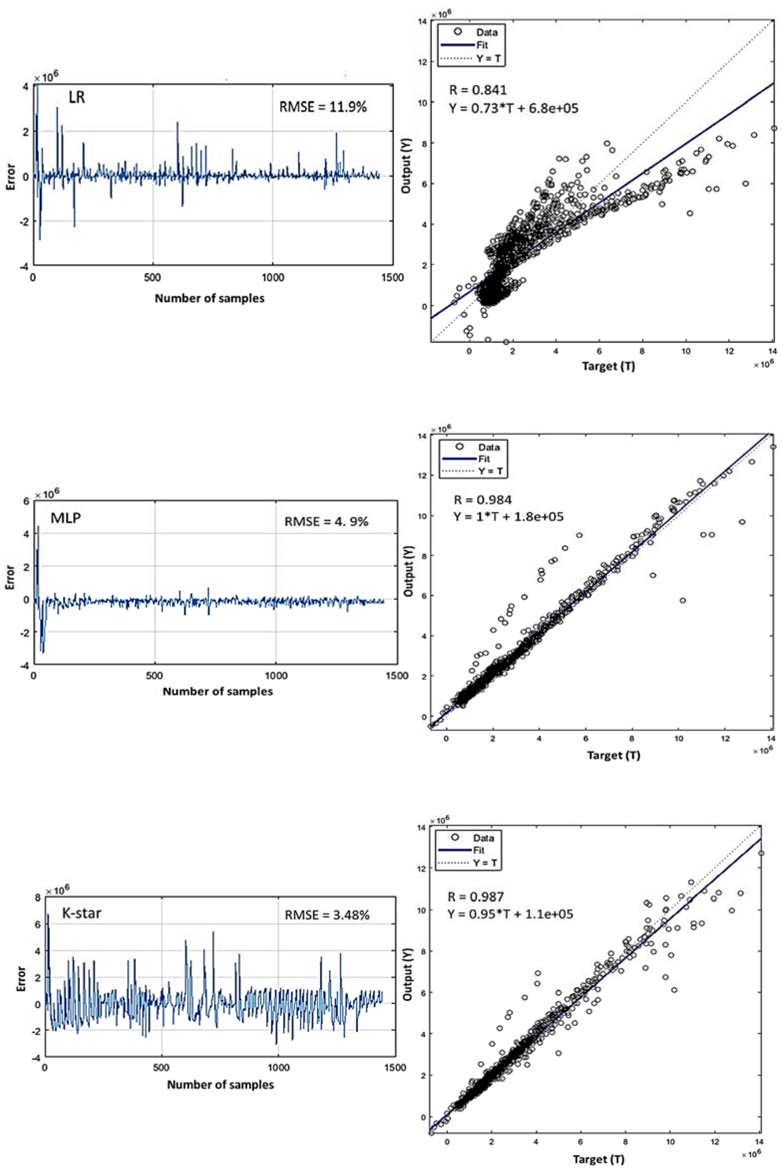
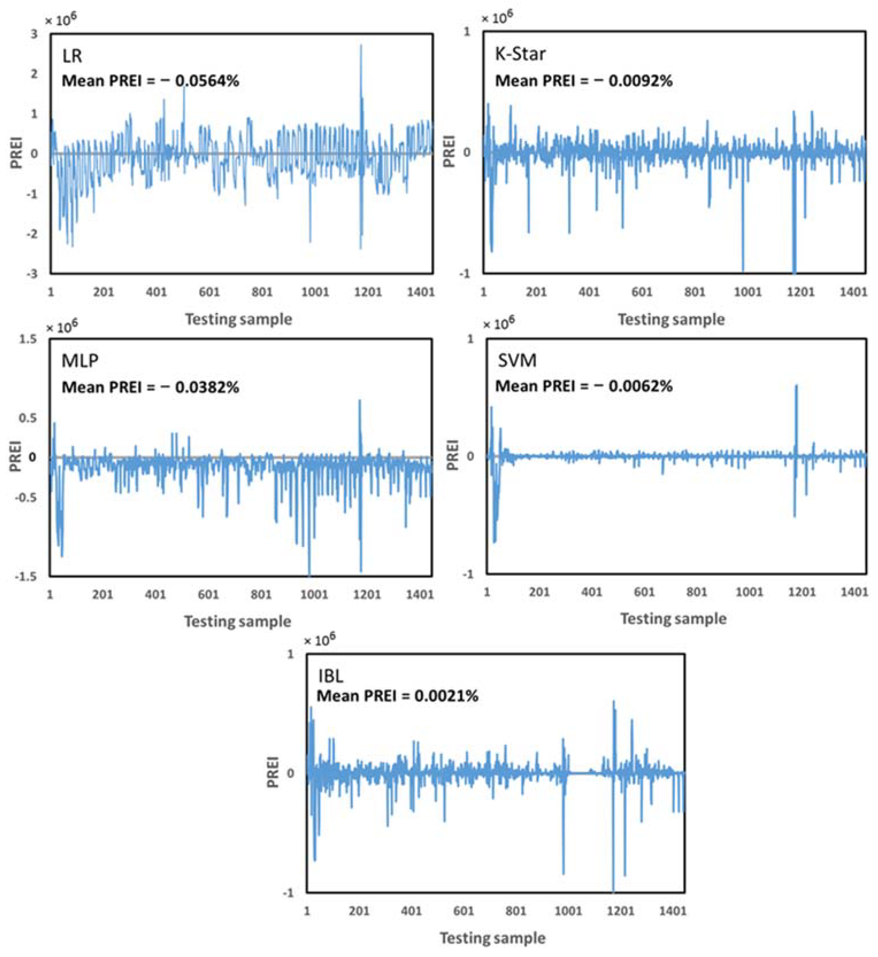
4. Results and Discussion

For all five models developed in this study, the magnitude of the modeling error was computed and comparative plots of target vs. output (i.e., actual cost vs. predicted cost) were prepared. Over the training phase (Figure 2), using the IBL model, the predicted costs were much closer to the actual values, indicating the greatest goodness of fit (RMSE = 1.4% and R = 0.998) to the training samples and to the linear regression equation: Y = T + 9.9e+03, in which Y is the model output (i.e., predicted total construction cost) and T is the cost reported in the project bids. In contrast, the LR model showed much farther predicted costs from the actual costs, yielding the highest training error (RMSE = 11.8%), the lowest R (0.834), and an equation of Y = 0.7T + 7.5e+05. The other three models used in this study were ranked from best to worst as, SVM (RMSE = 2.94% and R = 0.991), MLP (RMSE = 3.2% and R = 0.9894), and K-Star (RMSE = 3.4% and R = 0.988). The possible explanation for the superiority of IBL over the other models is that most of the variables (in particular, earth slope, size of trees, rock proportion of subsoil, and number of culverts) used in this study have great value distributions that make the search for neighboring instances easier for prediction purposes [39]. The most logical explanation for the low performance of the LR method compared to the other models is that LR assumes a predefined linear relationship between total cost and the independent variables. Although this assumption may yield promising results for other modeling studies, it seems that it does not fit the context of cost estimation modeling that is characterized by potentially very complex, nonlinear relationships.

The predictive power of the models could not be measured using the goodness of fit, because this metric uses the data with which the models were developed and shows only how well the models fit the training dataset. Conventionally, the predictive power of a model is measured via an external testing phase, during which the model is presented with unseen data [40]. The predictive power of our models was assessed over the testing phase that yielded the R values of 0.841 (LR), 0.984 (MLP), 0987 (K-Star), 0.993 (SVM), and 0.99 (IBL) (Figure 3). In terms of the magnitude of prediction error, the SVM model made the most accurate prediction (RMSE = 2.44%), followed by IBL (RMSE = 2.86%), K-Star (RMSE = 3.48%), MLP (RMSE = 4.9%), and LR (RMSE = 11.9%).

The highest generalization and predictive performances and capability to model nonlinear relationships using the SVM model can only be achieved if a suitable kernel function is utilized [41]. The kernel functions transform the nonlinear input space into a high dimensional feature space where nonlinear relationships and the solution to the problem are represented in a linear form [42]. Many different kernel functions exist that are used to create such high dimensional feature space. Since the nature of the real world data is typically unknown a prior choice among different kernels is impossible. Therefore, during the modeling process, different kernels are experimentally tried to find the one which gives the best performance. In this study, we evaluated the goodness of fit and predictive capability of the SVM model using four kernel functions based on the R, RMSE, and computing time (

Table 2. SVM performance with different Kernel types over the training and testing phases.

Phase	Metric	Kernel
		PK	NPK	RBFK	PUK
Training	R	0.825	0.974	0.846	0.991
	RMSE (%)	13.64	5.05	13.56	2.9
	Time (s)	13.14	26.12	17.32	50.37
Testing	R	0.834	0.982	0.854	0.993
	RMSE (%)	12.48	3.99	12.39	2.4
	Time (s)	13.17	26.37	17.92	49.07

Wherein: Time: time taken to build the model in seconds, PK: Poly Kernel, NPK: Normalized Poly Kernel, RBFK: Radial Basis Function Kernel, and PUK: Pearson Universal Kernel.

). Over the training phase, R ranged from 0.825 to 0.991 (mean = 0.909), RMSE ranged from 2.9% to 13.64% (mean = 8.79%), and time ranged from 13.14 to 50.37 s (mean = 26.74 s) that identified the PUK (R = 0.991, RMSE = 2.9%, time = 50.37 s) as the best kernel function for building the SVM model. Over the testing phase, R varied between 0.834 and 0.993% (mean = 0.916), RMSE varied between 2.4% and 12.48% (mean = 7.815%), and time varied between 13.17 and 49.07 s (mean = 26.63 s) that once again demonstrated the efficacy of PUK (R = 0.993, RMSE = 2.4%, time = 49.07 s) over the other kernel functions for the SVM model. The highest R and lowest RMSE achieved by PUK suggest that this kernel successfully grasped the relationship between different variables and construction cost. This efficacy stems from the flexibility of the PUK to adapt its two parameters from a Gaussian into a Lorentzian peak shape [42]. However, the SVM model with PUK still showed an RMSE of 2.9% and 2.4% that indicates the existence of some noisy sequences and bias in the datasets and the inability of PUK to avoid them.

Determining the number of neurons in the hidden layer is a crucial part of deciding the overall MLP architecture. To determine the optimum structure of the MLP model, the number of neurons in the hidden layer was investigated in a range of 1 to 50 neurons (Figure 4). The R, RMSE, and computing time obtained from the training dataset as input into the MLP model ranged from 0.9464 to 0.9894, 3.205% to 7.682%, and 0.75 to 21.16 s, yielding the best performance with 24 neurons in the hidden layer (R = 0.9894, RMSE = 3.205%, time = 10.03 s). Similarly, the model with 24 neurons performed in the testing phase (R = 0.9914, RMSE = 2.75%, time = 9.98 s) with an R, RMSE, and computing time that ranged from 0.9511 to 0.9914, 2.75% to 7.17%, and 0.76 to 20.5 s, respectively. The inefficiency of the MLP model with too few neurons in the hidden layer can be attributed to the underfitting problem [43] that hindered the MLP from adequately capturing the complicated relationships between the data leading to low model performance. However, structuring the MLP with too many neurons in the hidden layers excessively increased the computation time and may raise the overfitting problem in which the ANN model memorizes the idiosyncrasies of particular patterns between training samples and lost the generalization ability [43]. Our results clearly showed the increased computation time of the model by increasing the number of neurons in the hidden layer. Obviously, the MLP model with 24 neurons in the hidden layer offered a compromise between computation time and quality of results. Further, since the performance of the MLP model was within the range of other models developed in this study, we can conclude that the MLP with 24 neurons successfully overcame the overfitting problem.

As a further performance analysis, the PREI metric was computed and enabled us to examine the models based on their performance to underestimate or overestimate the construction cost (Figure 5). Except for the IBL model that overestimated the construction cost by 0.0021%, the other models underestimated the cost between −0.0062% (SVM) and −0.0564% (LR) than the actual cost available in the project bids. From these results, the LR model was identified as the most biased predictive model that underestimated the construction cost by −0.0564%. Underestimations and overestimations both negatively affect project management [44]. Underestimations may lead to poor quality of the deliverables and hence a bad reputation for the company [45].

In this case, the project managers may come to the conclusion that due to cost overruns and wasting resources and money the project should be stopped [46]. Overestimations can cause serious consequences, since the manager extends “the work so as to fill the time available for its completion” according to Parkinson′s Principal [47]. Apart from the reduced productivity rate, the overestimated budgets may lead the project manager to overlook a new contract to undertake new projects [45]. A survey on the literature related to infrastructure construction projects [48,49] shows a deviation towards underestimation of construction costs (i.e., cost overruns), which support our findings in this study. Ghajar et al. [1] also reported that the cost estimation models tend to underestimate the total construction costs of road projects in the Hyrcanian forests.

5. Conclusions

The task of cost estimation of road construction is one to which forest engineers have devoted much time and effort. In this study, we investigated the performance of different machine learning methods for the estimation of construction cost of forest road projects. We adopted a modeling methodology based on road project bids and field measurements to develop predictive models that enable forest engineers to estimate the construction cost of the next projects. Among the five models developed, the IBL model had the highest goodness of fit with the training dataset and the SVM model had the highest estimation capability. Except for the IBL model, which showed a cost overestimation of about 0.0021%, the other models slightly underestimated (0.0275%) the construction cost of forest roads. Based on the performance metrics and the costs reported in the project documentation, we found these machine learning models promising for estimating the total construction cost of forest roads. This study has opened up new avenues for machine-learning analyzing economic targets, management strategies, and system efficiencies that are undoubtedly important objectives of forestry enterprise. Future work could extend this analysis to the application of other machine learning methods as well as the application of metaheuristic optimization algorithms to automatically tune the methods′ parameters to produce more accurate cost estimation models.

References

1. Ghajar, I.; Najafi, A.; Karimimajd, A.M.; Boston, K.; Ali Torabi, S. A program for cost estimation of forest road construction using engineer’s method. For. Sci. Technol. 2013, 9, 111–117. [Google Scholar] [CrossRef]
2. Boston, K.; Leshchinsky, B.; Kemp, E.; Wortman, R. The use of a rotary asphalt broom to groom aggregate forest roads. Croat. J. For. Eng. 2017, 38, 119–126. [Google Scholar]
3. De Witt, A.; Boston, K.; Leshchinsky, B. Predicting aggregate degradation in forest roads in Northwest Oregon. Forests 2020, 11, 729. [Google Scholar] [CrossRef]
4. Sessions, J. Forest Road Operations in the Tropics; Springer: Berlin/Heidelberg, Germany; New York, NY, USA, 2007; 117p. [Google Scholar]
5. Bruce, J.C.; Han, H.-S.; Akay, A.E.; Chung, W. ACCEL: Spreadsheet-based cost estimation for forest road construction. West. J. Appl. For. 2011, 26, 189–197. [Google Scholar] [CrossRef] [Green Version]
6. Twito, R.H.; Reutebuch, S.E.; McGaughey, R.J.; Mann, C.N. Preliminary Logging Analysis Systems (PLANS), Overview; General Techincal Report PNW-199; USDA Forest Service: Portland, OR, USA, 1987; 24p.
7. Epstein, R.; Weintraub, A.; Sessions, J.; Sessions, B.; Sapunar, P.; Nieto, E.; Bustamante, F.; Musante, H. PLANEX: A system to identify landing locations and access. In Proceedings of the International Mountain Logging and 11th Pacific Northwest Skyline Symposium, Seattle, WA, USA, 10–12 December 2001; pp. 10–12. [Google Scholar]
8. Chung, W.; Sessions, J. NETWORK 2001—Transportation planning under multiple objectives. In Proceedings of the International Mountain Logging and 11th Pacific Northwest Skyline Symposium, Seattle, WA, USA, 10–12 December 2001; pp. 10–12. [Google Scholar]
9. Dykstra, D.P. Timber Harvest Layout by Mathematical and Heuristic Programming. Ph.D. Thesis, Department of Forest Engineering, Oregon State University, Corvallis, OR, USA, 1976. [Google Scholar]
10. Akay, A.E.; Boston, K.; Sessions, J. The evolution of computer-aided road design systems. Int. J. For. Eng. 2005, 16, 73–79. [Google Scholar] [CrossRef]
11. Akay, A.E. Minimizing total costs of forest roads with computer-aided design model. Sadhana 2006, 31, 621–633. [Google Scholar] [CrossRef] [Green Version]
12. Stückelberger, J.; Heinimann, H.R.; Chung, W. Improved road network design models with the consideration of various link patterns and road design elements. Can. J. For. Res. 2007, 37, 2281–2298. [Google Scholar] [CrossRef]
13. Meignan, D.; Frayret, J.-M.; Pesant, G.; Blouin, M. A heuristic approach to automated forest road location. Can. J. For. Res. 2012, 42, 2130–2141. [Google Scholar] [CrossRef]
14. Stückelberger, J.A.; Heinimann, H.R.; Burlet, E.C. Modeling spatial variability in the life-cycle costs of low-volume forest roads. Eur. J. For. Res. 2006, 125, 377–390. [Google Scholar] [CrossRef] [Green Version]
15. Markow, M.J.; Aw, W.B. Estimating road construction costs for sector planning in developing countries. Transp. Res. Rec. 1974, 898, 52. [Google Scholar]
16. Anderson, A.E.; Nelson, J. Projecting vector-based road networks with a shortest path algorithm. Can. J. For. Res. 2004, 34, 1444–1457. [Google Scholar] [CrossRef]
17. Heinimann, H.R. A computer model to differentiate skidder and cable-yarder based road network concepts on steep slopes. J. For. Res. 1998, 3, 1–9. [Google Scholar] [CrossRef]
18. Lucas, T.C. A translucent box: Interpretable machine learning in ecology. Ecol. Monogr. 2020, 90, e01422. [Google Scholar] [CrossRef]
19. Liu, Z.; Liu, Y.; Meng, Q.; Cheng, Q. A tailored machine learning approach for urban transport network flow estimation. Transp. Res. Part C Emerg. Technol. 2019, 108, 130–150. [Google Scholar] [CrossRef]
20. Samuel, A.L. Some studies in machine learning using the game of checkers. IBM J. Res. Dev. 1959, 3, 210–229. [Google Scholar] [CrossRef]
21. Clarviate. Web of Science Core Collection. 2020. Available online: https://clarivate.com/webofsciencegroup/solutions/web-of-science-core-collection/ (accessed on 15 November 2020).
22. Ghajar, I.; Najafi, A.; Torabi, S.A.; Khamehchiyan, M.; Boston, K. An adaptive network-based fuzzy inference system for rock share estimation in forest road construction. Croat. J. For. Eng. 2012, 33, 313–328. [Google Scholar]
23. Cleary, J.G.; Trigg, L.E. K*: An instance-based learner using an entropic distance measure. In Machine Learning Proceedings; Elsevier: Amsterdam, The Netherlands, 1995; pp. 108–114. [Google Scholar]
24. Hush, D.R.; Horne, B.G. Progress in supervised neural networks. IEEE Signal Process. Mag. 1993, 10, 8–39. [Google Scholar] [CrossRef]
25. Xu, Z.; Huang, X.; Lin, L.; Wang, Q.; Liu, J.; Yu, K.; Chen, C. BP neural networks and random forest models to detect damage by Dendrolimus punctatus Walker. J. For. Res. 2020, 31, 107–121. [Google Scholar] [CrossRef]
26. Cortes, C.; Vapnik, V. Support vector machine. Mach. Learn. 1995, 20, 273–297. [Google Scholar] [CrossRef]
27. Carrasco, M.; López, J.; Maldonado, S. A second-order cone programming formulation for nonparallel hyperplane support vector machine. Expert Syst. Appl. 2016, 54, 95–104. [Google Scholar] [CrossRef]
28. Aha, D.W.; Kibler, D.; Albert, M.K. Instance-based learning algorithms. Mach. Learn. 1991, 6, 37–66. [Google Scholar] [CrossRef] [Green Version]
29. Bui, D.T.; Khosravi, K.; Tiefenbacher, J.; Nguyen, H.; Kazakis, N. Improving prediction of water quality indices using novel hybrid machine-learning algorithms. Sci. Total Environ. 2020, 721, 137612. [Google Scholar] [CrossRef]
30. Jaafari, A.; Rezaeian, J.; Omrani, M.S. Spatial prediction of slope failures in support of forestry operations safety. Croat. J. For. Eng. 2017, 38, 107–118. [Google Scholar]
31. He, Y.; Dai, L.; Zhang, H. Multi-branch deep residual learning for clustering and beamforming in user-centric network. IEEE Commun. Lett. 2020, 24, 2221–2225. [Google Scholar] [CrossRef]
32. Jiang, L.; Zhang, B.; Han, S.; Chen, H.; Wei, Z. Upscaling evapotranspiration from the instantaneous to the daily time scale: Assessing six methods including an optimized coefficient based on worldwide eddy covariance flux network. J. Hydrol. 2021, 596, 126135. [Google Scholar] [CrossRef]
33. Bennett, N.D.; Croke, B.F.W.; Guariso, G.; Guillaume, J.H.A.; Hamilton, S.H.; Jakeman, A.J.; Marsili-Libelli, S.; Newham, L.T.H.; Norton, J.P.; Perrin, C.; et al. Characterising performance of environmental models. Environ. Model. Softw. 2013, 40, 1–20. [Google Scholar] [CrossRef]
34. Zhao, C.; Zhong, S.; Zhong, Q.; Shi, K. Synchronization of Markovian complex networks with input mode delay and Markovian directed communication via distributed dynamic event-triggered control. Nonlinear Anal. Hybrid Syst. 2020, 36, 100883. [Google Scholar] [CrossRef]
35. Mousavi, A.A.; Zhang, C.; Masri, S.F.; Gholipour, G. Structural damage detection method based on the complete ensemble empirical mode decomposition with adaptive noise: A model steel truss bridge case study. Struct. Health Monit. 2021, 14759217211013535. [Google Scholar]
36. Hu, B.; Wu, Y.; Wang, H.; Tang, Y.; Wang, C. Risk mitigation for rockfall hazards in steeply dipping coal seam: A case study in Xinjiang, northwestern China. Geomat. Nat. Hazards Risk 2021, 12, 988–1014. [Google Scholar] [CrossRef]
37. Adnan, R.M.; Jaafari, A.; Mohanavelu, A.; Kisi, O.; Elbeltagi, A. Novel ensemble forecasting of streamflow using locally weighted learning algorithm. Sustainability 2021, 13, 5877. [Google Scholar] [CrossRef]
38. Bie, Y.; Ji, J.; Wang, X.; Qu, X. Optimization of electric bus scheduling considering stochastic volatilities in trip travel time and energy consumption. Comput. Civ. Infrastruct. Eng. 2021, 1–19. [Google Scholar]
39. Ros, F.; Guillaume, S. From supervised instance and feature selection algorithms to dual selection: A review. Sampl. Tech. Superv. Unsuperv. Tasks 2020, 83–128. [Google Scholar]
40. Weis, C.V.; Jutzeler, C.R.; Borgwardt, K. Machine learning for microbial identification and antimicrobial susceptibility testing on MALDI-TOF mass spectra: A systematic review. Clin. Microbiol. Infect. 2020, 26, 1310–1317. [Google Scholar] [CrossRef] [PubMed]
41. Rahmati, O.; Jaafari, A. Spatial Modeling of Soil Erosion Susceptibility with Support Vector Machine. In Intelligent Data Analytics for Decision-Support Systems in Hazard Mitigation; Springer: Berlin/Heidelberg, Germany, 2021; pp. 267–280. [Google Scholar]
42. Üstün, B.; Melssen, W.J.; Buydens, L.M.C. Facilitating the application of Support Vector Regression by using a universal Pearson VII function based kernel. Chemom. Intell. Lab. Syst. 2006, 81, 29–40. [Google Scholar] [CrossRef]
43. Göçken, M.; Özçalıcı, M.; Boru, A.; Dosdoğru, A.T. Integrating metaheuristics and artificial neural networks for improved stock price prediction. Expert Syst. Appl. 2016, 44, 320–331. [Google Scholar] [CrossRef]
44. Mittas, N.; Angelis, L. Overestimation and underestimation of software cost models: Evaluation by visualization. In Proceedings of the 2013 39th Euromicro Conference on Software Engineering and Advanced Applications, Santander, Spain, 4–6 September 2013; pp. 317–324. [Google Scholar]
45. Briand, L.C.; Langley, T.; Wieczorek, I. A replicated assessment and comparison of common software cost modeling techniques. In Proceedings of the 22nd International Conference on Software Engineering, Limerick, Ireland, 4–11 June 2000; pp. 377–386. [Google Scholar]
46. Lederer, A.L.; Prasad, J. Causes of inaccurate software development cost estimates. J. Syst. Softw. 1995, 31, 125–134. [Google Scholar] [CrossRef]
47. Boehm, B.W. Software engineering economics. IEEE Trans. Softw. Eng. 1984, SE-10, 4–21. [Google Scholar] [CrossRef]
48. Bertisen, J.; Davis, G.A. Bias and error in mine project capital cost estimation. Eng. Econ. 2008, 53, 118–139. [Google Scholar] [CrossRef]
49. Callegari, C.; Szklo, A.; Schaeffer, R. Cost overruns and delays in energy megaprojects: How big is big enough? Energy Policy 2018, 114, 211–220. [Google Scholar] [CrossRef]
Figure 1. Flowchart of the modeling methodology adopted for cost estimation of road construction.
Forests 12 01169 g001
Figure 2. Model performance over the training phase.
Forests 12 01169 g002aForests 12 01169 g002b
Figure 3. Model performance over the testing phase.
Forests 12 01169 g003aForests 12 01169 g003b
Figure 4. MLP performance with the different number of neurons in the hidden layer over the training and testing phases. In each plot, the red-colored circle indicates the optimum number of neurons based on the highest R and lowest RMSE.
Forests 12 01169 g004
Figure 5. Error graph of the estimated cost compared to the actual cost reported in the project bids.
Forests 12 01169 g005