A Novel Method of Hyperbola Recognition in Ground Penetrating Radar (GPR) B-Scan Image for Tree Roots Detection

Abstract

Ground penetrating radar (GPR), as a newly nondestructive testing technology (NDT), has been adopted to explore the spatial position and the structure of the tree roots. Due to the complexity of soil distribution and the randomness of the root position in the natural environment, it is difficult to locate the root in the GPR B-Scan image. In this study, a novel method for root detection in the B-scan image by considering both multidirectional features and symmetry of hyperbola was proposed. Firstly, a mixed dataset B-Scan images were employed to train Faster RCNN (Regions with CNN features) to obtain the potential hyperbola region. Then, the peak area and its connected region were filtered from the four directional gradient graphs in the proposed region. The symmetry test was applied to segment the intersecting hyperbolas. Finally, two rounds of coordinate transformation and line detection based on Hough transform were employed for the hyperbola recognition and root radius and position estimation. To validate the effectiveness of this approach for tree root detection, a mixed dataset was made, including synthetic data from gprMax as well as field data collected from 35 ancient tree roots and fresh grapevine controlled experiments. From the results of hyperbola recognition as well as the estimation for the radius and position of the root, our method shows a significant effect in root detection.

1. Introduction

As an important part of the Earth’s ecosystem, the tree plays a positive role in dealing with soil erosion and adjusting climate. Most roots, which are the main organ for absorbing nutrients and for physical support, are underground [1,2]. Because of the opacity of the soil and the complexity of the root spatial structure, the study for roots lags far behind that of other organs of the tree. In recent years, ground penetrating radar (GPR), a new nondestructive geophysical exploration technology, has been widely used in the field of material detection such as in minerals and civil engineering applications [3,4,5]. Compared to traditional root nondestructive detection methods like Electrical Resistance Tomography [6,7] (ERT) and Ultrasonic Pulse Velocity Analysis [8,9,10,11] (UPV), GPR is employed to explore the spatial structure of the root [12,13] because it is efficient, accurate, simple to operate, and high-resolution. It not only promotes research on roots but also provides the related data for tree protection and engineering construction.

Owing to the difference of the relative permittivity between the tree roots and the soil, the roots usually appear in a hyperbola pattern [14,15] in radar B-Scan images obtained from the GPR. So, the root detection is transformed into the recognition of the hyperbola pattern in the B-Scan image. The traditional interpretation of the B-Scan image requires experts with relevant expertise, which is inefficient and difficult to generalize. In the past decade, some researchers proposed processing methods including the techniques of signal processing, image processing, and machine learning for hyperbola detection in B-Scan images. These methods are roughly summarized in three steps [16,17,18,19]: (1) pre-process B-Scan image to reduce the influences of the noise, system effect, and other influence factors; (2) segment image to search for the potential hyperbola region; and (3) distinguish the hyperbola from the candidate area.

In the actual environment, there are often many noises in the B-Scan image caused by the randomness of the soil distribution, the radar hardware, and wave interactions. These factors bring many difficulties to hyperbola recognition. Thus, some signal processing and image processing methods are applied to preprocess the B-Scan image such as removing direct wave, filtering, and adjusting gain. Wen et al. [20] presented shearlet transform to denoise the B-Scan image and achieved higher scores in several image evaluation criteria including the peak signal-to-noise ratio (PSNR), the signal-to-noise ratio (SNR), and the edge preservation index (EPI) than in wavelet, contourlet, and curvelet [21] transform. To obtain the regions which might contain the hyperbola, these researchers [22,23,24] adopted manual threshold, boundary threshold, and edge detection to process the preprocessed image [25] after signal processing [26,27] into a binary image. To detect the hyperbola region with machine learning, Mass et al. [28] adopted Viola-Jones (VJ) [29] to extract hyperbola regions and Pasolli et al. [16,30] designed a method based on Genetic Algorithm (GA) and adopted Support Vector Machine (SVM) to classify the binary region. With the growth of data volume, the traditional learning methods based on manual features show their shortcomings. Deep learning, a new learning algorithm without predefined features, develops rapidly. Some experts [31,32,33,34,35,36,37] proposed hyperbola detection methods with Convolutional Neural Network (CNN) [38]. Pham et al. [39] and Lei et al. [40] employed Faster RCNN (Regions with CNN features) [41], a two-stage object detection framework based on CNN. To separate and recognize the hyperbola from the extracted regions, Dou et al. [42] proposed the column connection clustering (C3) algorithm to segment hyperbola from the binary image and classified the segmentation by the neural network. Zhou et al. [23] considered the down-open characteristic of the hyperbola and proposed an open-scan clustering algorithm (OSCA) to obtain the hyperbola points set, then classified the set by a hyperbola feature, and finally used the restricted algebraic-distance-based fitting (RADF) algorithm to fit a hyperbola by calculating algebraic distance. Lei et al. [40] proposed the double cluster seeking estimate (DCSE) and column-based transverse filter points (CTFP) methods to depart the hyperbola area and fitted the hyperbola based on the potential hyperbola region proposed by Faster RCNN. In these studies [22,24,26,43,44,45,46], the redesigned Hough transform and Least Squares (LS) methods by the hyperbola characteristic were used to detect the hyperbola. Liang et al. [47] estimated the root diameter on gprMax data.

Because of the change of the relative permittivity underground, there are many visible response areas in the radar B-Scan image. In the on-site B-Scan image, the areas like the boundaries of the air–soil and the soil–root show obvious responses. The previous methods made use of the change of A-scan signal at a single detection point in the vertical direction and ignored the difference between adjacent multiple detection points in the horizontal direction. As for separating the intersecting hyperbolas, these methods focused on the connectivity and opening direction without considering the symmetry of the hyperbola. In addition, the results of this framework mainly depend on binary images. The general threshold calculation could be influenced by the outliers that would cause the binary images, ignoring some local change and losing the corresponding information.

In this study, we paid attention to the characters in both the detection direction and scanning direction and introduced symmetry to separate multiple crossed hyperbolas. A novel method of hyperbola recognition for root detection in GPR B-Scan image was proposed. This method can be divided into three parts: hyperbola region detection, connected region extraction, and hyperbola recognition. In the first part, the mixed dataset which is comprised of the synthetic data from the gprMax toolbox [48] and field data from GPR was used to train the Faster RCNN model with three different backbone networks. After that, the hyperbola region were obtained from the trained models. Secondly, the image gradient and connected component analysis were employed to obtain the peak area and the tail area of the hyperbola, and segment the connected region for each top area by symmetry after matching the peak area and the tail area. Finally, the line detection with Hough transform was applied after making coordinate transformations by the key point on the hyperbola. The radius and position of the root was estimated by the parameters of the simplified equation.

2. Theoretical Basis of the Root Detection Method

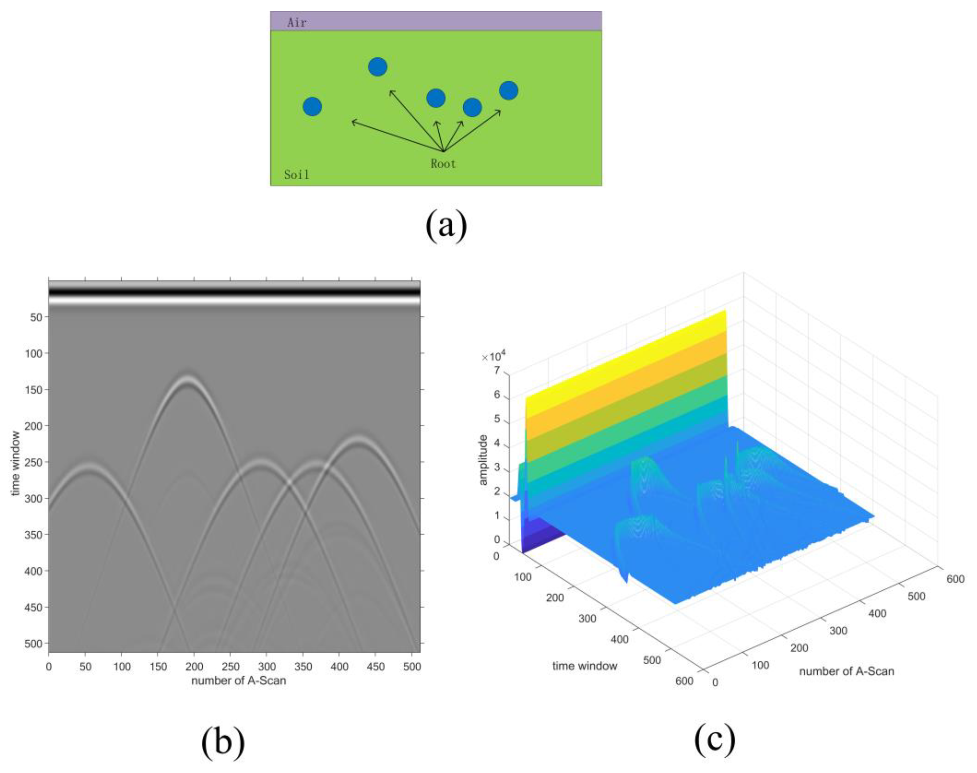
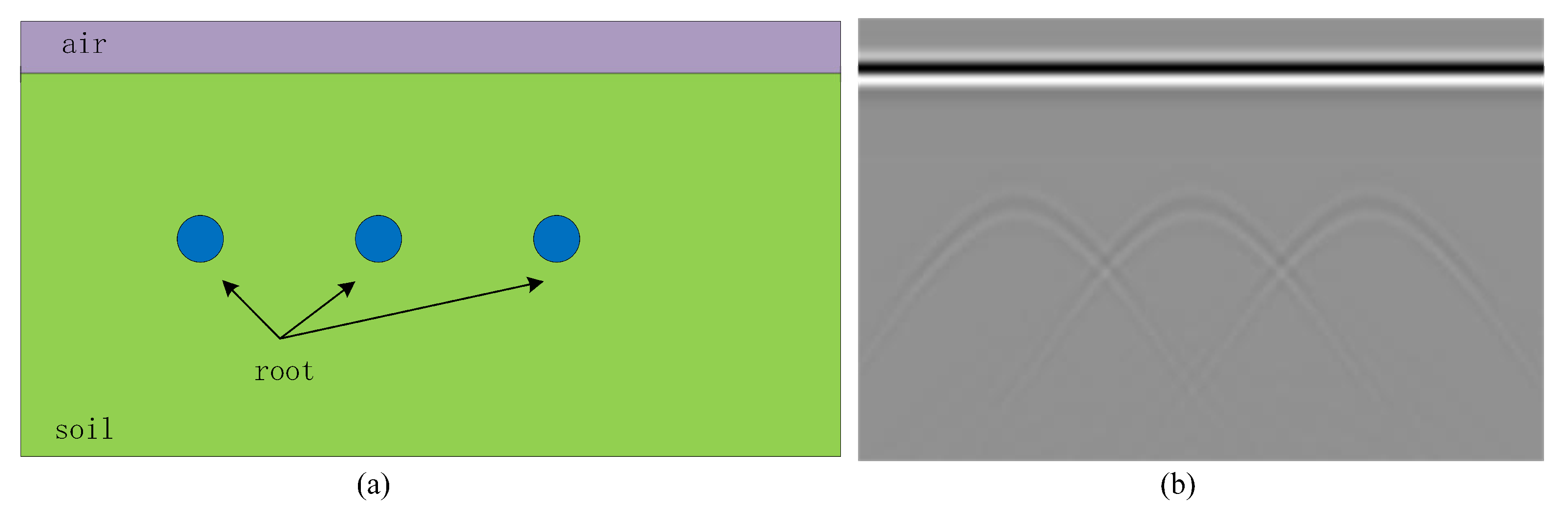
The radar B-Scan image is composed of multiple A-Scan signals by continuously scanning the tangent plane of a certain position of the tree root system using GPR. From the regional distribution perspective, the B-Scan image could reflect the distribution of media on the scanning plane, such as the upper region of the air–soil boundary and the hyperbola region of the root system at the corresponding position. Due to the different relative permittivity and the position of these mediums, the corresponding area in the radar wave data not only appears in different time-depth but also shows varying degrees of change. In the B-Scan image, these regions have different changing characteristics in scan direction at the same time. In Figure 1, an example of the synthetic model from simulation data generated by gprMax, its B-Scan image, and amplitude graph were shown. In this example, the domain is 0.6 m in depth and 2.5 m in length, the discretization of space in the x, y, and z directions is 0.002 m respectively as well as the radius of the roots is 0.01 m. The relative permittivity values of the domain and root are 6 and 12 [49,50,51]. As for the set-up for the GPR, the antenna frequency is 900 MHz and the sampling number is 512. In Figure 1a, there are five roots with the same radius in the geometric models. Two of the roots are farther apart and the other three are closer together. As shown in Figure 1b, the interface of the air–soil appears as a direct wave and the roots show hyperbola pattern. There are two relatively independent hyperbolas and three intersecting hyperbolas. In Figure 1c, the B-Scan image is converted into the 3D amplitude graph to observe the characteristics from the perspective of the change of response. By comparing the three graphs, two interesting conclusions could be summarized. The first is the boundaries of the air–soil and soil–root have obvious amplitude changes in the corresponding position and in the detecting direction. The other is the amplitude change in the scanning direction does not change significantly compared with the detection direction in the same area. In detail, the electromagnetic wave emitted by GPR shoots from the air into the soil and the soil into the root in the vertical direction. Because it travels through different media, an obvious response was found at the boundaries of the two media. At the same time, because of the same distance between the radar and the boundaries in the scanning direction for each A-Scan, the changes of the amplitude appear at about the same detection time.

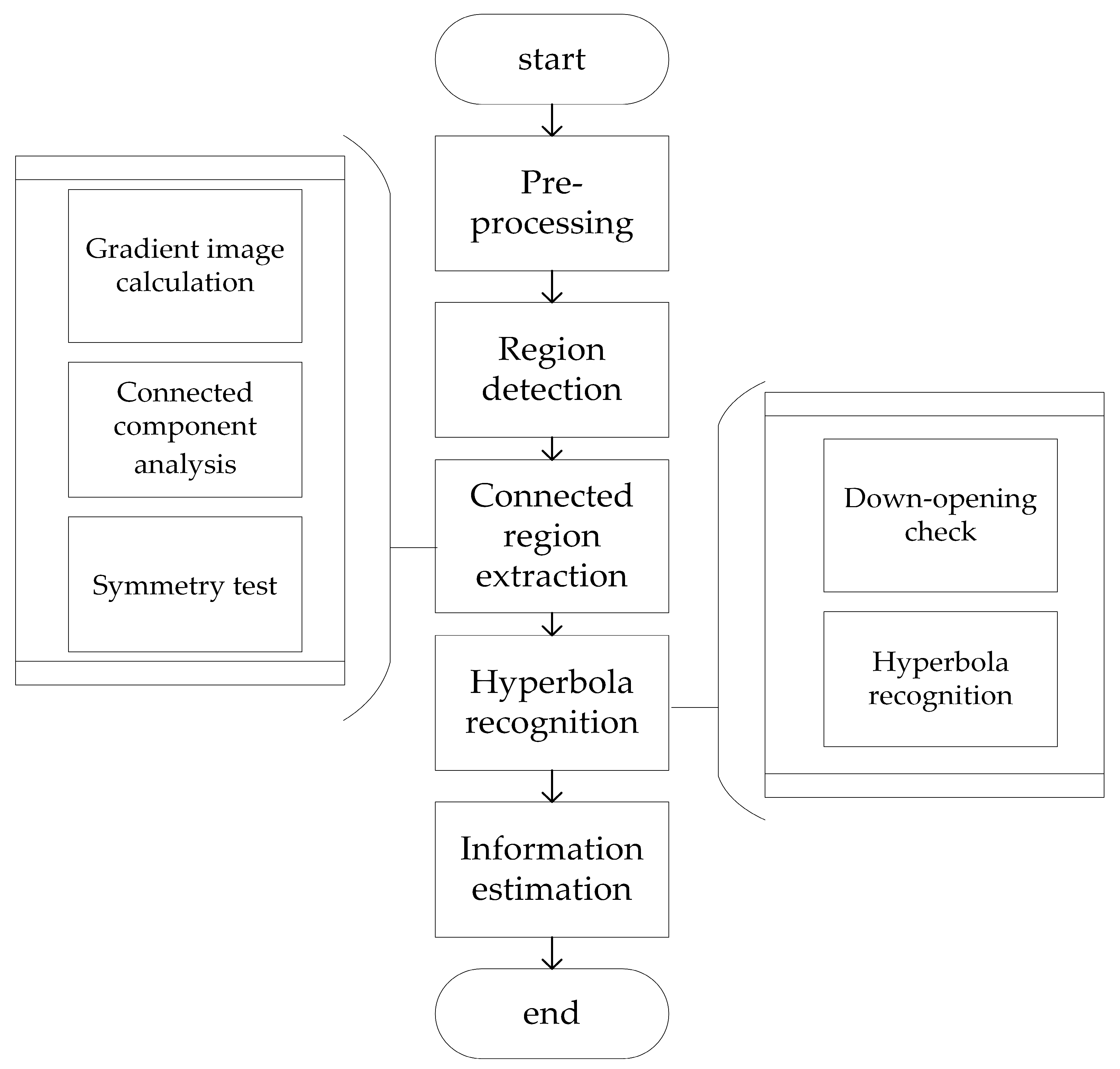
To capture these changes, the image gradient which describes the change of an image in a certain direction for image processing was adopted. A novel method for root detection in GPR B-Scan image was proposed based on the difference of the changes in the horizontal and vertical image gradients. Figure 2 shows the flow chart of our method, mainly including three stages for hyperbola region detection, connected region extraction, and hyperbola recognition. In the first stage, Faster RCNN, an object detection framework, was employed to detect the potential hyperbola regions. Based on the proposal region, there were image gradient calculations and symmetry tests in the next stage. In the last stage, coordinate conversions for each symmetrically connected region were made twice by taking the key point from its peak to the down-opening, and checked for hyperbola recognition, by adopting Hough transform to fit the hyperbola and estimate the radius and position of the root. In this section, all these three phases are described in detail.

2.1. Hyperbola Region Proposition via Faster RCNN

Every scanning tangent plane of GPR often has several roots with random positions owing to the complexity of the root distribution. There are multiple hyperbolas in the B-Scan image but they only occupy a small part of the whole image. Some approaches for hyperbola recognition involve calculating on the whole B-Scan image directly, so much calculating time is required on the area without hyperbola. If the calculation could focus on the hyperbola region, the effectiveness of recognition would improve significantly. However, it is also hard to fix the parameters of the window size and slide step for the traditional approach, slide window, due to the difference in the hyperbola pattern. The template matching method is often constrained by the hyperbola template library. In recent years, with the development of deep learning, some algorithms-based neural network for object detection made a breakthrough like RCNN, YOLO, SSD, and their variants [41,52,53,54,55,56,57,58]. Although the one-stage approach had a surprising detection speed, it was slightly less accurate than the two-stage method with twice the adjustments due to the whole process adjusting the proposed region only once. With the region proposal network (RPN) proposed, the part of the generation of the proposal region was accelerated by the GPU. That meant the two-stage approach could achieve nearly real-time detection.

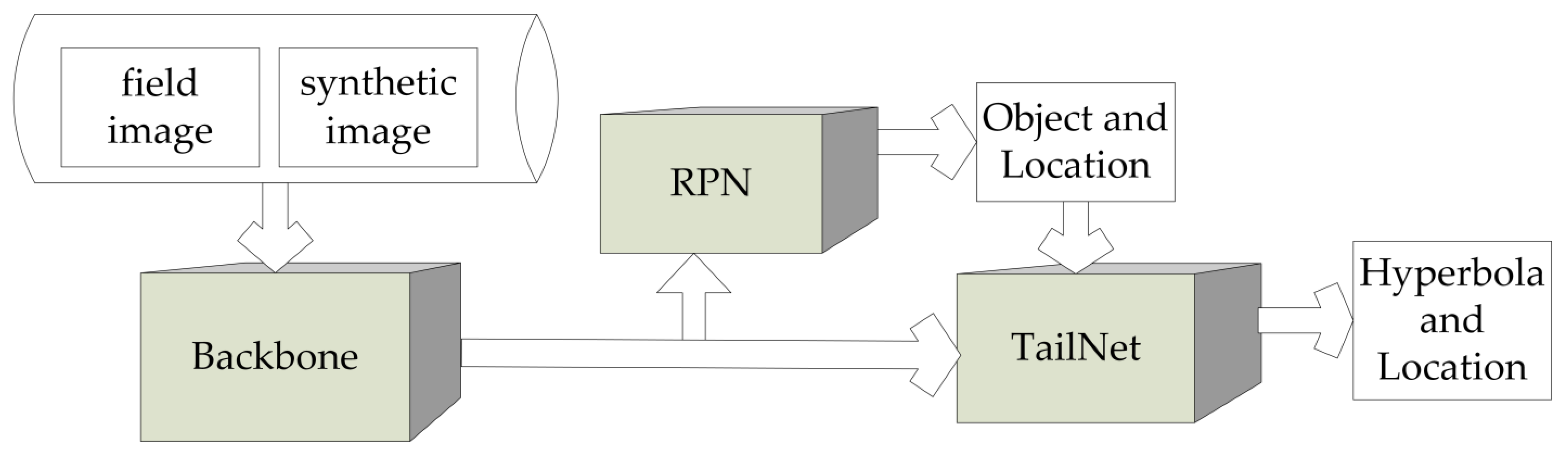
For hyperbola detection of B-Scan images, it is necessary to reduce detection time as much as possible while ensuring high accuracy. Thus, we adopted Faster RCNN, a two-stage framework with three different backbone networks to detect the hyperbola region. Figure 3 shows the framework for obtaining hyperbola regions with Faster RCNN. For feature extraction, we adopted three backbone networks: vgg16, resnet50, and resnet101. The the feature map was sent into the RPN and regression network. Finally, the proposal box for the hyperbola with location and confidence was generated.

2.2. Peak and Tail Extraction of the Hyperbola

In the B-Scan image, when the radar wave passes through the interface of two media with different relative permittivity, there is an obvious amplitude fluctuation. The surface of the soil shows a transverse zonal region and the root in the scanning tangent plane usually shows the hyperbola shape. Figure 1 shows a root model from simulated data for its radar B-Scan image and amplitude diagram obtained from the gprMax tools. From the vertical perspective, the B-Scan image is composed of many A-Scan signals. In each A-Scan signal, there is obvious amplitude fluctuation at the detection time corresponding to the air–soil and soil–root interfaces. From the horizontal perspective, the B-Scan image was viewed in different moments. There is little change at the moments corresponding to the interfaces of the air–soil and the small area at the top of the soil–root, but there are obvious changes at the time corresponding to other parts of the soil–root boundary.

2.2.1. Longitudinal and Transverse Gradient Graphs Calculation

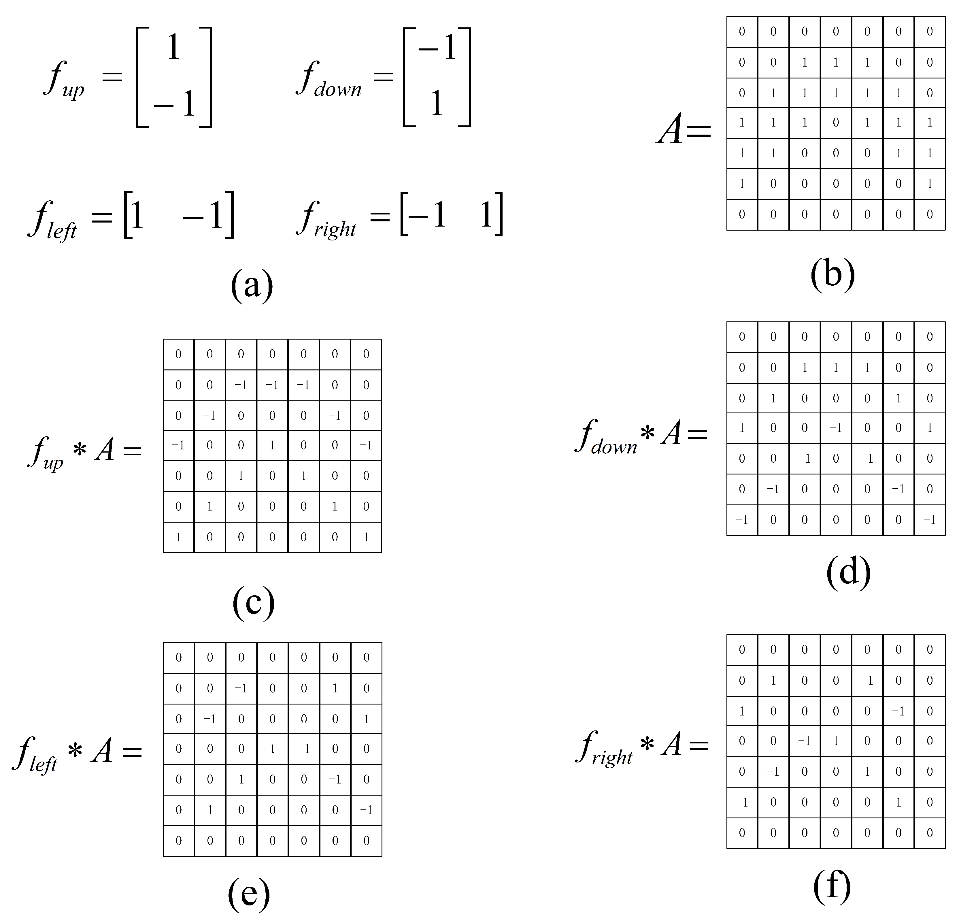
Image gradient is used to describe the change in one direction of the image by using a pre-defined descriptor and making a convolutional operation on an image. Although large size descriptors could make use of multiple pixels in adjacent positions and reduce the influence of the noise point, the template is too large to capture the difference of two adjacent pixels. Figure 4 shows the pre-defined simple difference descriptors and an example for calculating the gradient graph in four directions. In Figure 4a, there are four different descriptors. The example, image $A,$ is shown by pixel value in Figure 4b. In Figure 4c–f, the upward, downward, left, and right gradient graphs are shown after the convolutional operation with the corresponding descriptor.

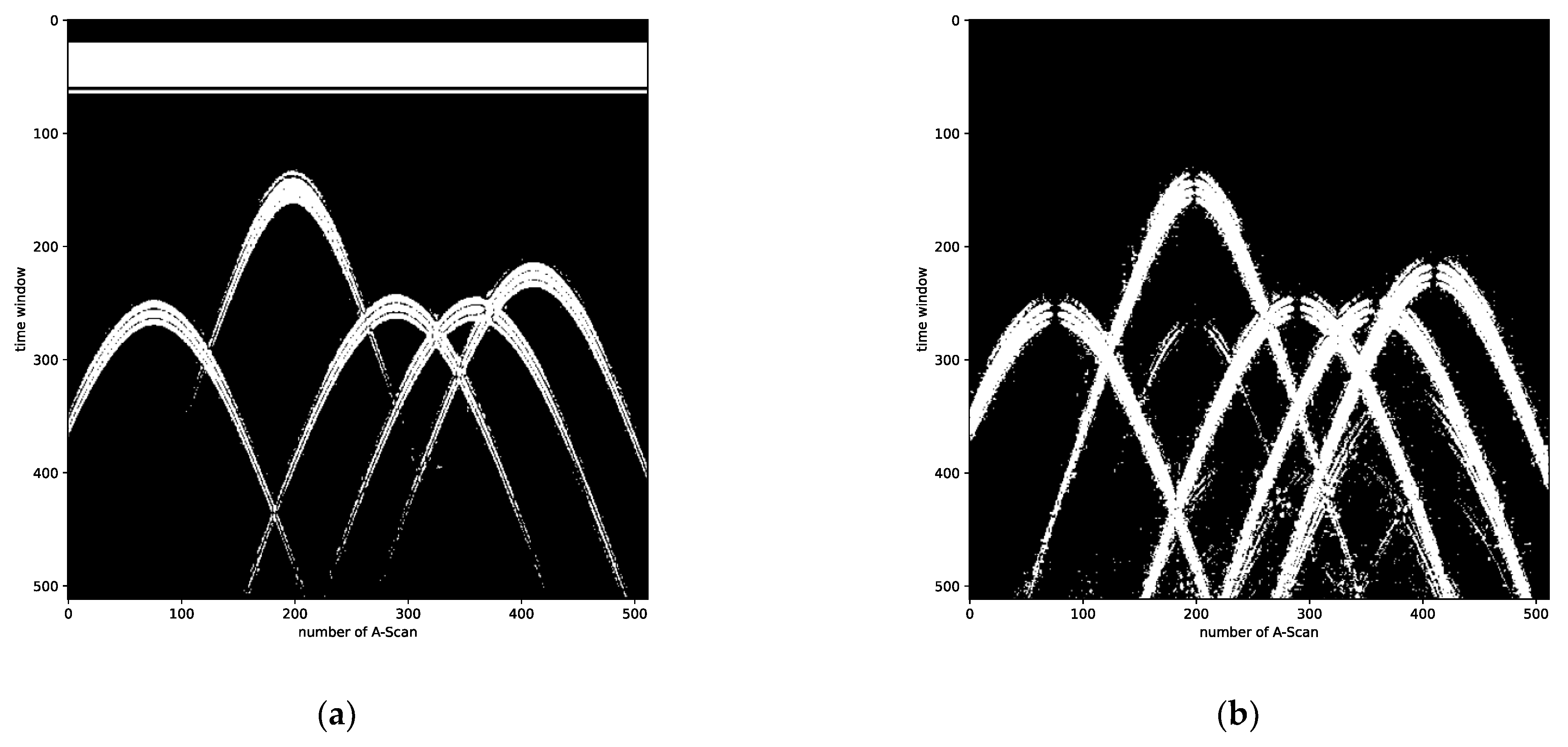
In this study, four simple small size descriptors were pre-defined in Figure 4 to calculate the difference in the up, down, left, and right directions of the B-Scan image. To make use of these features, we combined the gradient images in four directions acquired by making convolution operations into longitudinal and transverse gradient graphs after binarization by the gradient value as shown in Figure 5. In the longitudinal gradient map, there are some areas which correspond to the interface of the air–soil and soil–root existing at a non-zero gradient. It also has some discrete regions caused by noise. In the other graph, the gradients of the boundaries of the air–soil and small area at the top of the soil–root approach to zero. Other regions of the soil–root interface still have a non-zero gradient. Through morphological analysis, the interface of the air–soil approximates a straight zonal region in the scanning direction. From the vertical direction, the amplitude fluctuation is caused by the difference between air and soil. From the horizontal direction, the amplitudes are approximately equal at the same time. Thus, the interface of the air–soil appears in the vertical gradient graph, not in the other graph. The scanning cross-section of the root appears similar to the circular shape and the amplitude fluctuation at a different time in the several adjacent corresponding A-Scan signals and shows the hyperbola shape in the B-Scan image combined with those A-Scan signals. However, in the horizontal direction of viewing, the top small area of the root is approximately a horizontal straight line which is similar to the former. Hence the gradient is close to zero in that area and there is a non-zero gradient in other regions of the hyperbola. In the two gradient graphs, the whole hyperbola shape was found in the vertical gradient graph, but only two tails for each hyperbola appear in the horizontal gradient graph lacking the top small area.

2.2.2. Connected Component Analysis

There are some noises in both gradient graphs appearing in a discrete small area. However, some noisy regions could not be eliminated by dilation and erosion with the small kernel. Although these morphological operations with a large kernel could remove these regions, the different features of the top of the hyperbola in longitudinal and transverse gradient graphs would be influenced. Hence the connected component analysis, one of the morphological image processing methods was adopted to eliminate the discrete noisy region. This method could mark every region in an image that could not be absorbed by other regions after dilation and erosion. The connected component is usually used to describe the region composed of foreground pixels with the same pixel value and adjacent position in the image with a connected structure descriptor. 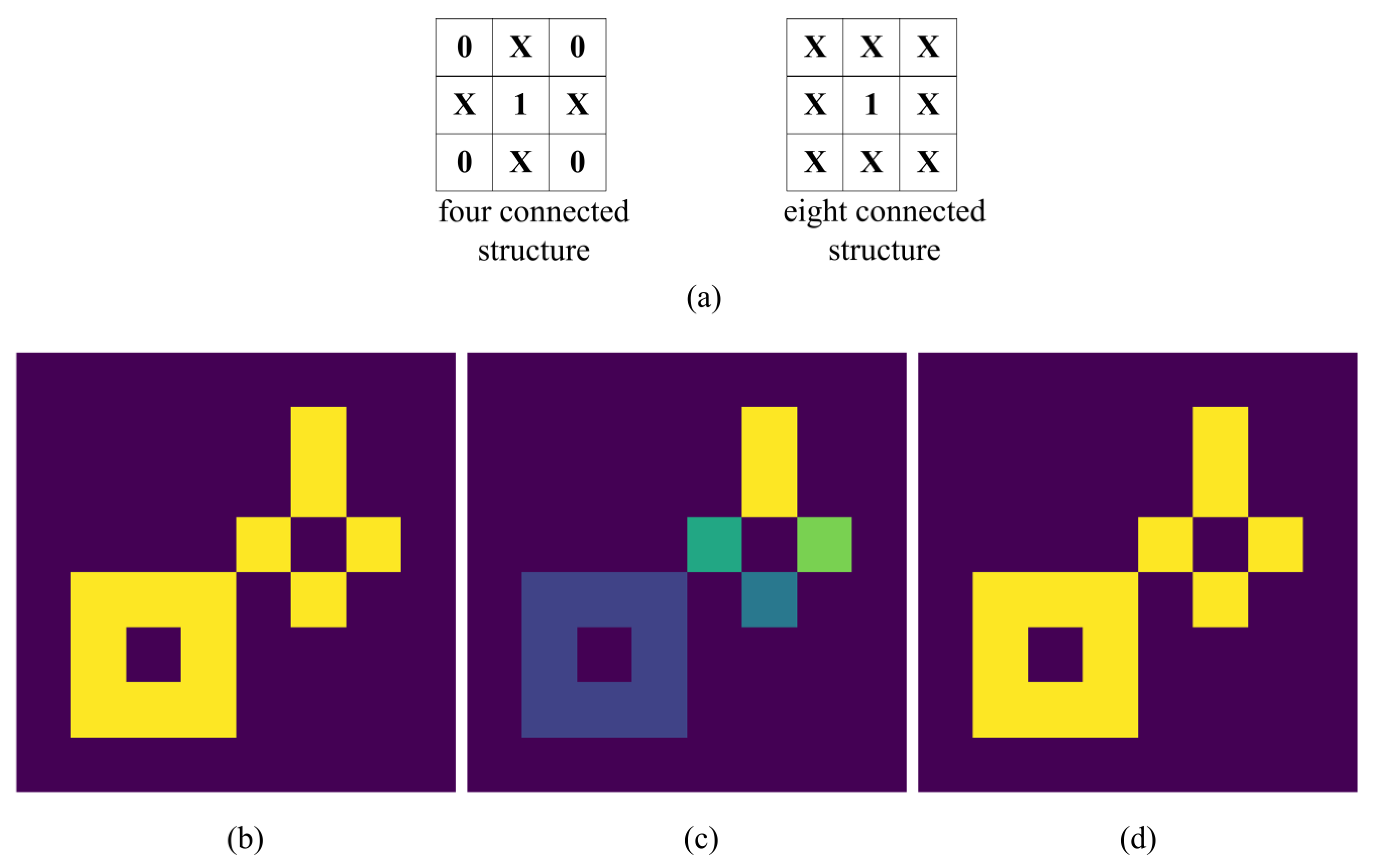Figure 6 shows a simple example of the connected component analysis with the four-connected structure and eight-connected structure. In Figure 6a, the two types of connected structures are shown. The example image (the yellow area is the foreground and the rest is the background) is shown in Figure 6b. Figure 6c,d show the results after connected component analysis with the four-connected structure and eight-connected structure respectively. In these results, the same color shows the same region. There are five regions in Figure 6c and only one region in Figure 6d. From these two kinds of connected structures and the corresponding results, the analysis results include the diagonal position of the point with the eight-connected structure. In this study, the eight-connected structure was predefined to do the connected component analysis of the vertical and horizontal gradient graph and a threshold for eliminating the noisy region was calculated on the average area of all the connected components by Equation (1). The result after denoising by the connected component analysis is shown in Figure 7.

$${\mathrm{Area}}_{\mathrm{avg}}=\frac{1}{\mathrm{n}}{\displaystyle \sum }_{\mathrm{i}=1}^{\mathrm{n}}{\mathrm{area}}_{\mathrm{i}}$$

(1)

2.2.3. Symmetry Test

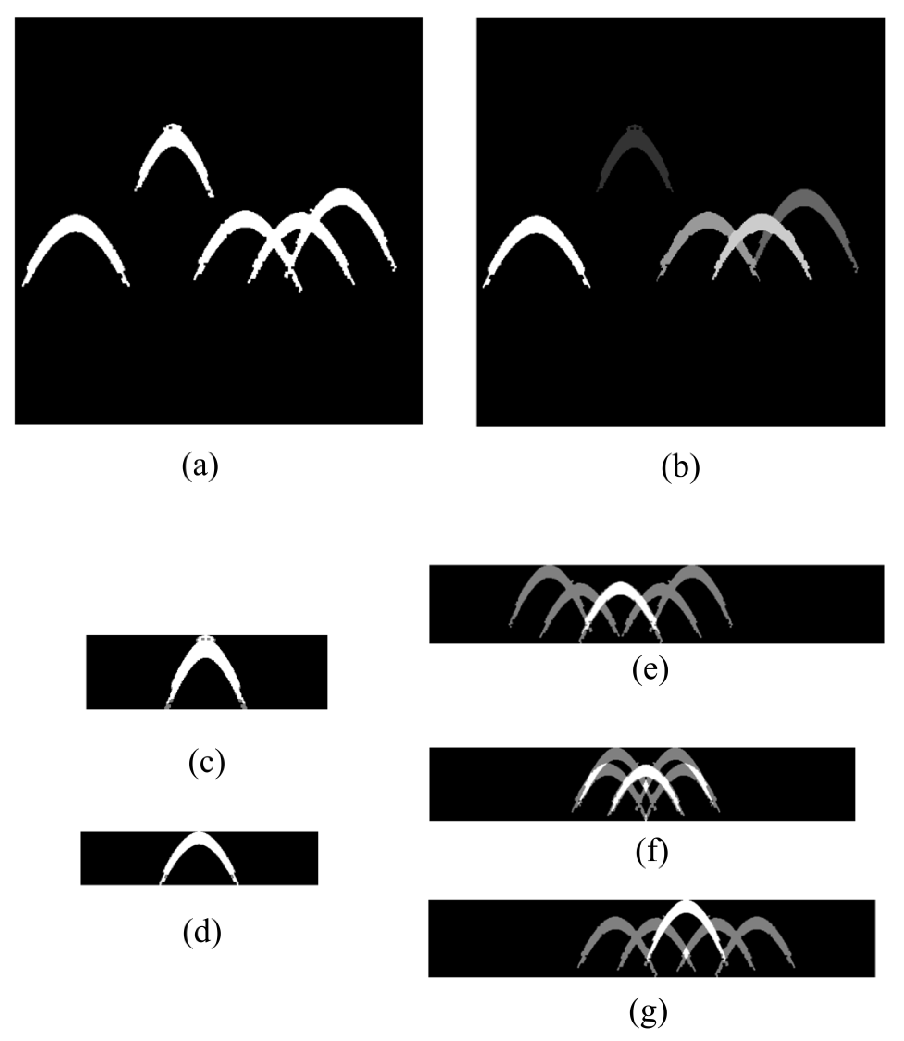
In the radar B-Scan image, the root usually shows a hyperbola shape with symmetry caused by the principle of detection with GPR. For each root, the corresponding hyperbola is symmetrical about the A-Scan at the highest point. Comparing the longitudinal and transverse gradient graphs, the top area of each hyperbola area shows differently. In the vertical direction, the hyperbolas keep the complete shape. However, in the horizontal direction, only the two tail regions are reserved without the top area. The top area was obtained by image linear operation and matched with the connected components by position. The symmetry test was applied to separate each corresponding connected component into independent symmetric regions with every matched top area. 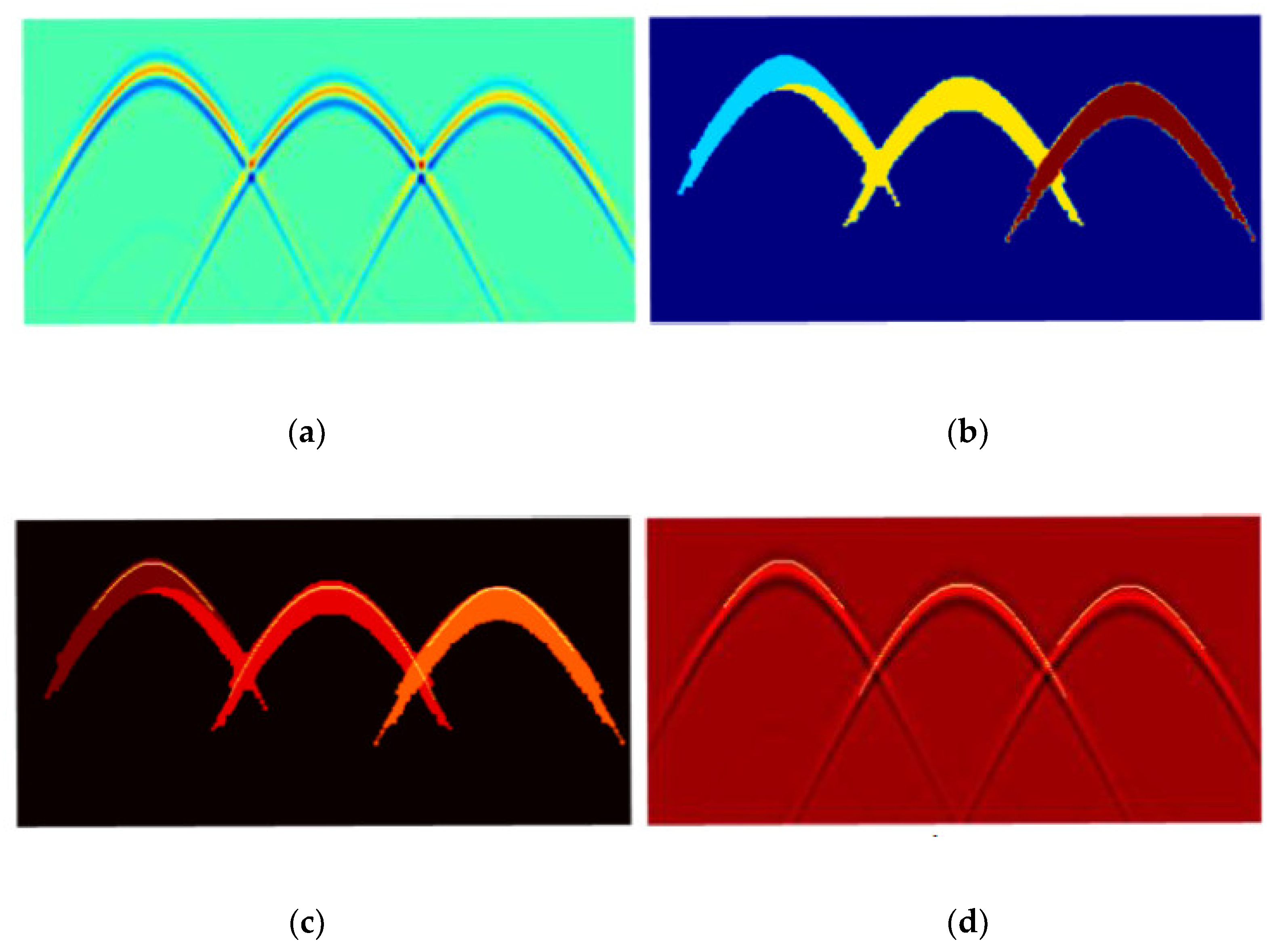Figure 8 shows the results of this test on a simulation image. In the results, two independent hyperbolas were preserved and the three intersecting hyperbolas were separated into three independent hyperbolas with three top areas. The connected component analysis was also employed to retain the symmetry region which determined the corresponding top area in the intermediate process.

2.3. Key Point Coordinate Transformation for Hyperbola Recognition

After separating symmetric regions, the Least Squares and Hough transform are employed to fit the hyperbola from the regional points. The former is usually used for equation fitting with a known point set of one single hyperbola. There are some restrictions in this method: (1) the point set must be the hyperbola pattern; (2) the point set could only contain one hyperbola; and (3) the result is easily affected by noise points. Hough transform is a method that uses a point set to vote and cluster in parameter space to determine the equation. It is not necessary to determine the morphological characteristics of point sets in advance and as they could be composed of multiple hyperbolas. In this method, the threshold of voting points in parameter space is used to determine whether or not there are hyperbolas and the number of hyperbolas in the point set. The previous method of hyperbola detection using Hough transform simplified the hyperbola equation based on the GPR imaging principle and voted in a three-dimensional Hough space. That caused a large amount of calculation and high computational complexity because of the high parameter dimension. Due to the discretization of the infinite continuous parameter domain, there is a deviation for hyperbola recognition. In this study, the separated symmetric connected region and its top area were obtained by using the difference of the hyperbola between the longitudinal and transverse gradient graphs. Therefore, the location of the vertex was used as a priori knowledge to further simplify the hyperbola equation and detect the hyperbola in the separated symmetric connected region. The simplified hyperbola equation was transformed into a linear equation by coordinating transformation based on the location of the vertex. The hyperbola detection of the origin set was transformed into line detection in new coordinates, which could reduce the dimension of parameter space and convert the infinite continuous parameter domain to finite by polar coordinate transformation.

2.3.1. Down Opening Check with Key Point

The root usually shows the circle in the scanning plane and appears a hyperbola pattern in the corresponding GPR B-Scan image. After extracting the symmetric connected region, the feature points of the hyperbola are selected by a downward opening check for each region and used for hyperbola fitting. The hyperbola is similar to a parabola with some same points. Therefore, parabola detection was adopted for the downward opening check to gain some key points where hyperbola and parabola coincide. Some identical transformations were applied on the parabola Equation (2) and a linear Equation (4) was obtained based on the axis of symmetry with Equation (3).

$$y=a_0+a_1\times {\left(x-a_2\right)}^2$$

(2)

$$X={\left(x-a_2\right)}^2$$

(3)

$$y=a_0+a_1\times X$$

(4)

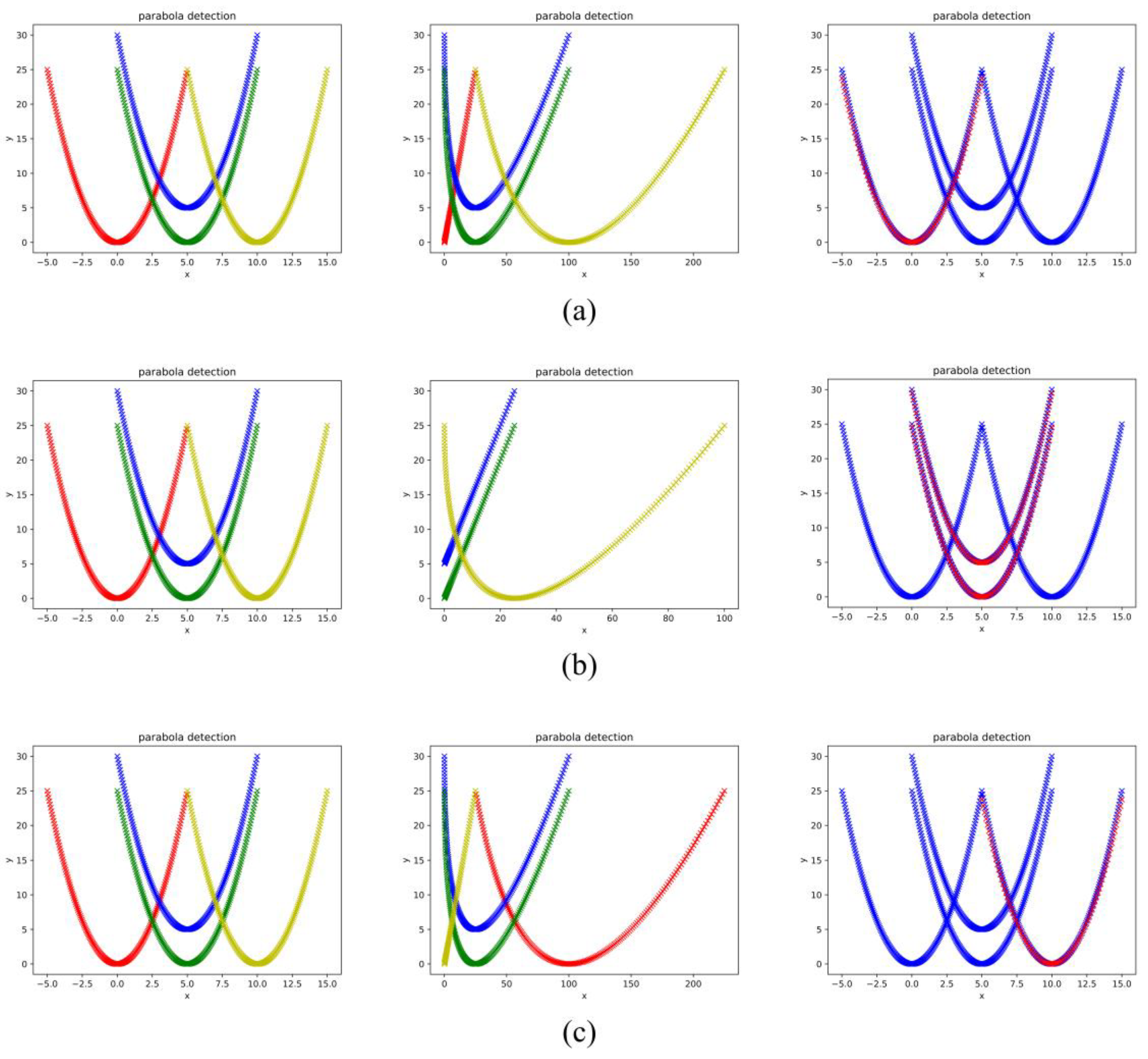
Figure 9 shows some examples of parabola detection by line detection with Hough transform after one coordinate transformation. In the first column, the red curve is a parabola for which the equation is $y=x^2$, the green and the yellow are the road moved right 5 and 10 units, respectively, and the blue is the green moved up 5 units. The second column is the result after coordinate transformation with $a_2=0$, $a_2=5,$ and $a_2=10$. The third column is the result of line detection by Hough transform on the point set in the second column. In the third column, the blue curve is the original curve and the red curve is the detected curve. From the results, the parabolas with different symmetry axes were fitted after coordinate transformation with the corresponding symmetry axis. The parabolas with the same symmetry axes were fitted after coordinate transformation with the common symmetry axis. In the downward opening check on the B-Scan image, the parameter $a_0$ and $a_1$ should be positive.

2.3.2. Hyperbola Recognition with Key Point and Root Parameters Estimation

The root showing the hyperbola signature in B-Scan image was formulated as a geometric model [19,59,60] as shown in Figure 10. Equation (5) expresses the relation of the scanning time $t$, the horizontal position $x$, the velocity of propagation $\nu$ and the radius of the root $R$.

$${\left(\frac{t+\frac{2R}{v}}{t_0+\frac{2R}{v}}\right)}^2+{\left(\frac{x-x_0}{\frac{v}{2}\times t_0+R}\right)}^2=1$$

(5)

where ($x_0,t_0$) are the coordinates of the target and $\left(x,t\right)$ are the coordinates of the points on the hyperbola. Equation (6) is the standard equation of the hyperbola. After some simple derivations with Equation (5), the relations in Equations (7) and (8) were obtained.

$${\left(\frac{y-y_0}{a}\right)}^2-{\left(\frac{x-x_0}{b}\right)}^2=1$$

(6)

$$a=t_0+\frac{2R}{v}$$

(7)

$$b=\frac{v}{2}\times \left(t_0+\frac{2R}{v}\right)$$

(8)

If the parameters of the hyperbola, $a$ and $b,$ were searched, the depth, the radius of the root, and the propagation velocity of electromagnetic wave were calculated by Equations (9)–(11) at the same time.

$$R=\frac{b\times \left(a-t_0\right)}{a}$$

(9)

$$depth=\frac{v\times t}{2}=\frac{v\times t_0}{a}$$

(10)

$$v=\frac{2b}{a}$$

(11)

Transform Equation (5) with $a$, $b$ and obtain a new Equation (12) without parameters $v$ and $R$.

$${\left(\frac{t+a-t_0}{a}\right)}^2-{\left(\frac{x-x_0}{b}\right)}^2=1$$

(12)

In this equation, there are still four parameters $a$, $b$, $t_0$, and $x_0$. The former methods regarded this problem as an optimization problem to solve the optimal solution. The parameters $t_0$ and $x_0$ are the coordinates of the hyperbola vertex. In this study, the top area of the hyperbola was obtained from the vertical and horizontal gradient graphs as the prior knowledge. So, let

$$X={\left(x-x_0\right)}^2\hspace{1em}y=t-t_0\hspace{1em}t=y+t_0$$

(13)

and make some identity transformations from Equation (14).

$${\left(y+a\right)}^2=a^a+\frac{a^2}{b^2}\times X$$

(14)

$$y^2=\frac{a^2}{b^2}\times X-2\times a\times y$$

(15)

If y > 0, Equation (16) was deduced which was regarded as a linear Equation (17).

$$y=\frac{a^2}{b^2}\times \frac{X}{y}-2\times a$$

(16)

$$y=a_0+a_1\times Z$$

(17)

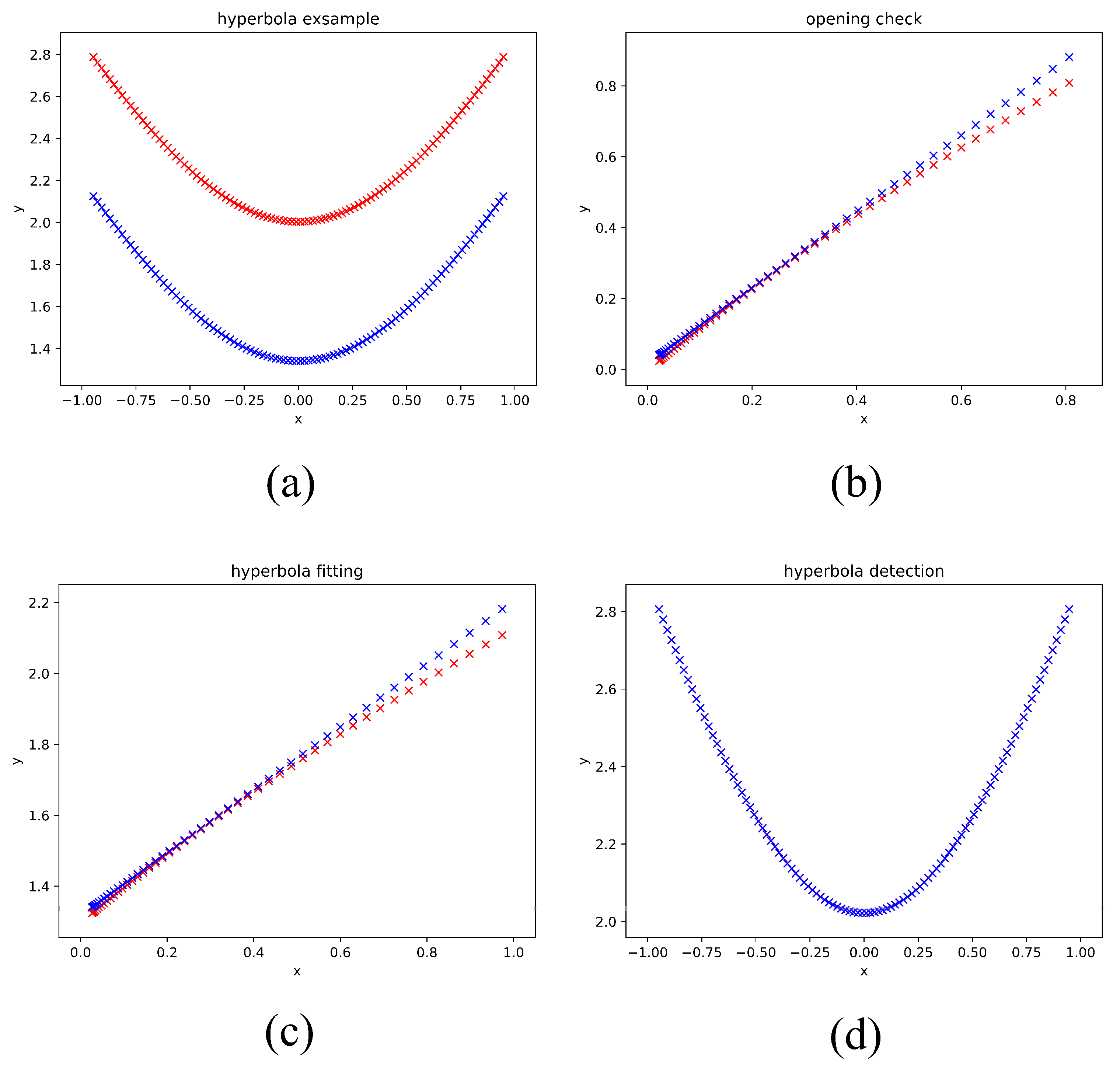
After the transformation with key point, an equation with four parameters was simplified into a linear equation with only two parameters. The linear detection method with Hough transform was adopted to estimate the two key parameters of Equation (17). A simple example for hyperbola fitting with Hough transform is shown in Figure 11. In Figure 11a, the red curve is a simple hyperbola for which the equation is $\frac{y^2}{a^2}-\frac{x^2}{b^2}=1$, when $a=2$, $b=1$. The blue curve is the red curve moved down 1.2 units. Figure 11b,c show the intermediate results of the down opening check and hyperbola fitting for the blue curve in Figure 11a. In these two figures, the red curve is to be fitted and the blue is the fitting result. From the result, a fine hyperbola fitting and accurate parameter estimation were obtained using our method.

This section shows the novel method for root detection in the GPR B-scan image by considering the horizontal and vertical characteristics and the symmetry of the hyperbola. From the results of theoretical analysis and numerical validation, this method could not only recognize a single hyperbola but also separate multiple intersecting hyperbolas. To test and verify the effectiveness of our method for tree root detection, standing tree root system, grapevine controlled experiment, and numerical simulation data were collected.

3. Materials and Methods

3.1. Materials

Our study situ was located in Summer Palace, a landscape with a temperate monsoon climate in the western suburb of Beijing. There are hundreds of ancient trees with huge and complex roots. Tree root detection by GPR could provide important data support for the protection of these ancient trees. In our experiments, 35 trees located in the flat meadow and open environments were selected, including willows, pines, and cypresses. The grapevine, which has a similar relative permittivity to the root, was chosen in the controlled experiment.

3.2. Field Detection of Standing Trees and Embedded Roots

According to the characteristics of the root system and combined with previous experience in tree detection, the TRU tree radar (SIR3000T, GSSI, USA) was employed. The tree radar detection system was combined with a radar wave medium coupling single polarized antenna and a data collector. At the same time, the trace-interval and the number of samples are 5 mm and 512, respectively. In the field experiment, the antenna frequency was 900 MHz and the detecting depth was 0.6 m. Due to lateral roots radiating outward from the taproot, the root orientation was usually unknown before digging. To ensure a quasi-perpendicular intersection with most of the roots, a method of loop detection was adopted [12]. An example for tree root detection is shown in Figure 12. In our detection, the tree trunk was regarded as the center circle in the detection design. The detection started from due north and ran counterclockwise. The tracks were circulars around the trunk and increased by 0.4 m each time from 0.6 m to the longest distance of the crown. To date, we have detected the root system of 35 ancient trees and collected 409 DZT files.

Furthermore, to verify the validity of both the field experimental data and simulation data, a controlled experiment was designed and detected in the Practice Base (40°29″ N, 116°20′27″ E) of Beijing Forestry University. This region has a temperate continental monsoon climate with four distinct seasons and its coverings are mainly fine sand. There is no significant difference in the permittivity between the fine sand and soil, and the physical properties are uniform. The experimental field is 2 m long, 1 m wide, and 0.6 m deep, as shown in Figure 13. This shows an experiment for roots with different radius. The depth and distance of these roots are 0.3 m and 0.5 m. The detection direction is perpendicular to the embedded root system and the track was a straight line. Owing that the aim of this paper is to detect the root of the living standing ancient tree, the newly excavated grapevine was chosen in the control experiment to get as close as possible to the real detection.

3.3. Numerical Simulation of Root with Random Position

To enumerate multiple positional relationships of roots, the gprMax3.0 toolbox, an open-source software that could simulate electromagnetic wave propagation by finite-difference time-domain (FDTD) method was employed to generate the synthetic images. The relative permittivity of the sand and soil with 20 percent water content were about 4 and 10, respectively, and the relative permittivity of the root was about 12 [49,50,61]. GPR B-Scan image was best in dry sandy soils but seriously degraded in soils with high water and clay contents [62]. The soil in the natural environment (not after rain) was more homogeneous and biased towards dry soil, and root detection using GPR mainly used the difference in the relative permittivity of the soil and the root system. The detection depth and GPR resolution, including the minimum size detectable as well as the capacity to discriminate between two closely-spaced targets [62], are influenced by the antenna [12]. High-frequency antenna has high resolution but low detection depth, and low-frequency antenna has high penetration but low resolution. This paper used a 900 MHz antenna, whose maximum detection depth was about 1 m [63], the diameter of the smallest detectable root was about 2 cm [64], and the detectable smallest interval between closely-located roots was between 10 and 20 cm [65].

In order to simulate the real environment as much as possible, the base model is shown in Figure 14, which includes the air and soil regions by the following setting: the detection domain was 0.6 m for vertical depth, 6 m for lateral length, and 0.002 m for section thickness. The air layer was 0.04 m, the antenna frequency is 900 MHz, the relative permittivity of the root and soil was between 11-to-13 and 6, respectively, and the start positions of the transmitting antenna and receiving antenna were 0.004 m and 0.008 m for the lateral position. There are several cylinders as root models whose random radius was from 0.01 m to 0.035 m with the random location in the soil box and the distance to each one was greater than five times the radius. After simulation, several technologies like pepper noise and Gaussian blur were applied to the images to be similar to the real images.

In this section, the mixed dataset was prepared to verify the effectiveness and accuracy of the method for root detection in B-Scan images. Some approaches of image processing like mean filter, median filter, Gaussian filter, gain adjustment, expansion, and corrosion were adopted to preprocess the B-Scan images.

4. Results and Discussion

4.1. Analysis of Hyperbola Region Proposition

The framework of Faster RCNN was split into three parts: the backbone, RPN, and tail networks. The VGG16, ResNet50 and ResNet101 were employed as the backbone network for feature extraction. In order to train the whole network effectively, the weights of these networks trained by the ImageNet dataset were loaded to initialize the backbone network weight. The Pascal VOC2007, a classical dataset of object detection with 20 classes was adopted to pre-train the whole model. After that, our mixed B-Scan dataset after random data augmentation was used to fine-tuning the weight trained on Pascal VOC2007. The technology for data augmentation includes image scaling, stretching, flipping, clipping, and gain adjusting. The whole program was implemented with PyTorch, an open-source deep learning framework. The training phase was run on a server equipped with Nvidia Titan XP GPU and the test phase was on a personal laptop with Intel i7-9750H and Nvidia GTX1660ti. As for model evaluation, mean average precision (mAP) and frames per second (FPS) were employed the measure the precision and time consumption. The mAP is commonly used to evaluate the precision of the object detection algorithm by considering both the confidence and intersection over union (IoU) of the object and the FPS usually shows the detection speed that not only depended on the algorithm efficiency but also influenced by the computer hardware platform.

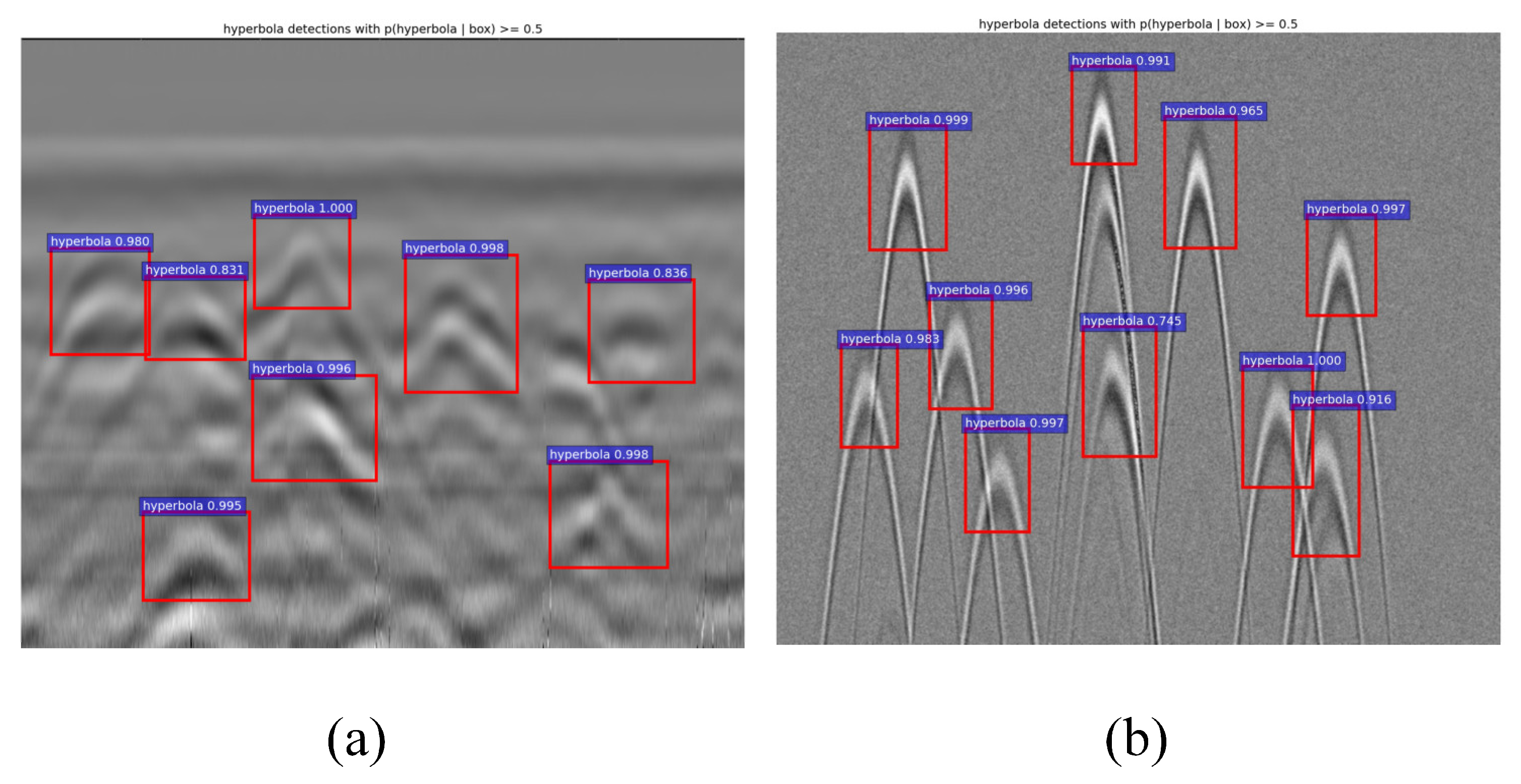
The whole mixed dataset includes 1442 images (1160 for synthetic images and 282 for on-site images). The dataset was divided into 80% for training, 10% for verification and the remaining 10% for test. As for training, the three models were trained for 50 epochs respectively. In Figure 15, one on-site and one synthetic image after detecting are shown. From the result, most hyperbolas are detected but there are still several undetected hyperbolas due to the complex noise, weak response, and hyperbola interaction. After training, the mAP, time pre-image (TPI), and FPS of the three models for hyperbola detection were calculated and compared as shown in

Table 1. The comparison for the mAP, TPI and FPS of three different backbone networks.

Backbone Network	VGG16	ResNet50	ResNet101
mAP	84.94%	86.67%	89.71%
TPI	0.987 s	1.273 s	1.662 s
FPS	1.02	0.79	0.62

. From the table, the mAP is higher but the TPI is longer and the FPS is less with the increase of network layers. Due to the increased network layers, the backbone network could extract more effective features but cause more calculation. Therefore, precision would increase with the deeper network but more would require more time. In this study, the model with resnet101 was adopted by considering both the detection accuracy and time consumption.

4.2. Analysis of Hyperbola Extraction

In this part, the simulation data was used to verify the connected region extracting method for segmenting the intersecting hyperbolas in the B-Scan image firstly. The root position in the simulation model was generated randomly, so the data produced by the gprMax software includes many relationships of the hyperbolas such as lambda shape and x shape. The gradient graphs in four directions and the symmetry test were adopted to do hyperbola segmentation in various forms whose connected regions include a single hyperbola and multiple hyperbolas with intersecting.

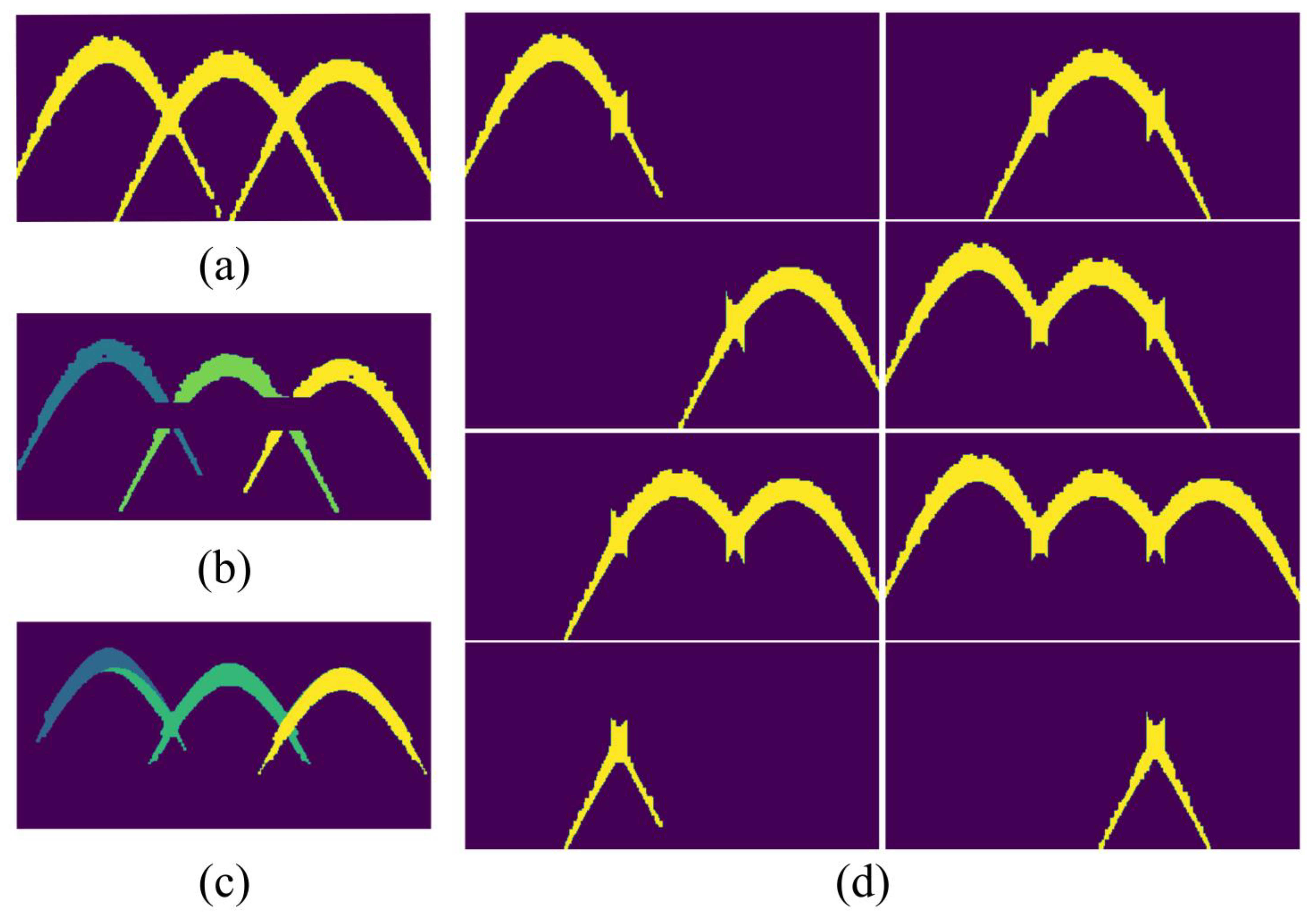
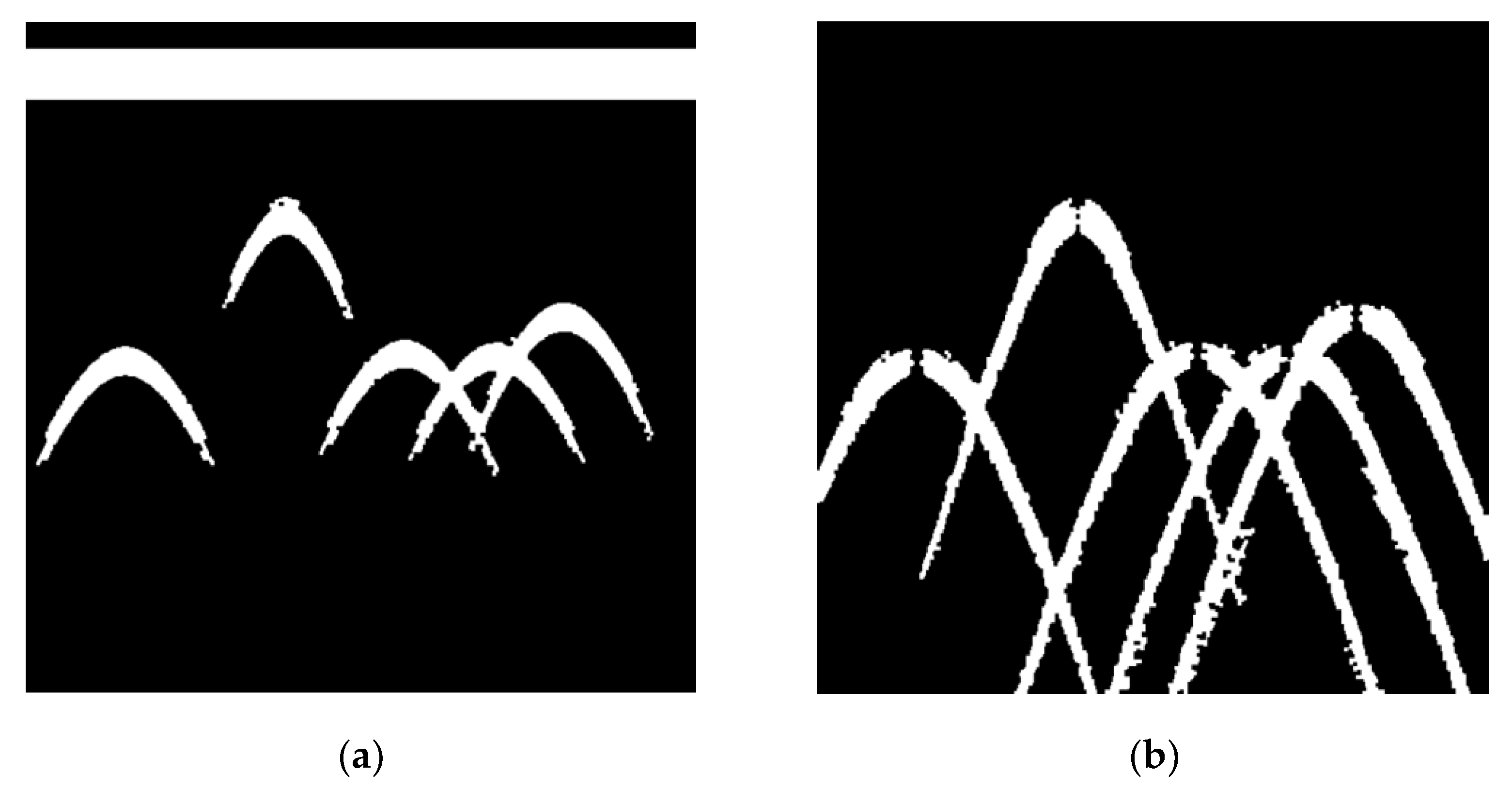
Figure 16 compares the results after the B-Scan image segmentation with C3, OSCA, and our method. In Figure 16a, there is an example image with three intersecting hyperbolas. Figure 16d shows the clustering result for the connected region including three hyperbolas by C3, and there are eight clusters in total. The segmentation process of C3 was clustered by two important definitions: the column segment and connecting elements. The output of this approach included not only the hyperbola shape but also other shapes owing to the interaction of multiple hyperbolas. The number of clustering results was dependent on the number of consecutive crossed hyperbolas. Hence a hyperbola judging method was employed to filter the clustering results following the segmentation phase. Figure 16b shows the output of the OSCA algorithm for the same connected region. The process of OSCA considered three overlapping patterns like lambda, x, and v shape, and segmented them by two definitions, the point segment and the downward/upward opening. If there is a hole in the connected region that would be regarded as an x shape, the clustering result would be influenced. In this experiment, a simple trick considering the gap between two point segments dependent on the size of the hole was adopted to correct the shape judgment. The C3 and the OSCA were influenced by the rough edge of the connected region, noise, and the internal hole of the region. Figure 16c shows the output of our symmetry test. In this experiment, the hyperbolas on both sides could keep the whole shape but the middle one was affected by its intersecting. Owing to the two sides roots with approximate depth and offset value to the middle one, some region in the hyperbolas on both sides is symmetric to the middle root. Therefore, the segmentation result for the middle hyperbola would include some regions from the sides. Figure 17 shows the result of the hyperbola recognition on this segmentation. From the output, all three hyperbolas were distinguished respectively. Although there were some interference areas in the middle hyperbola, our method could still recognize the hyperbola robustly.

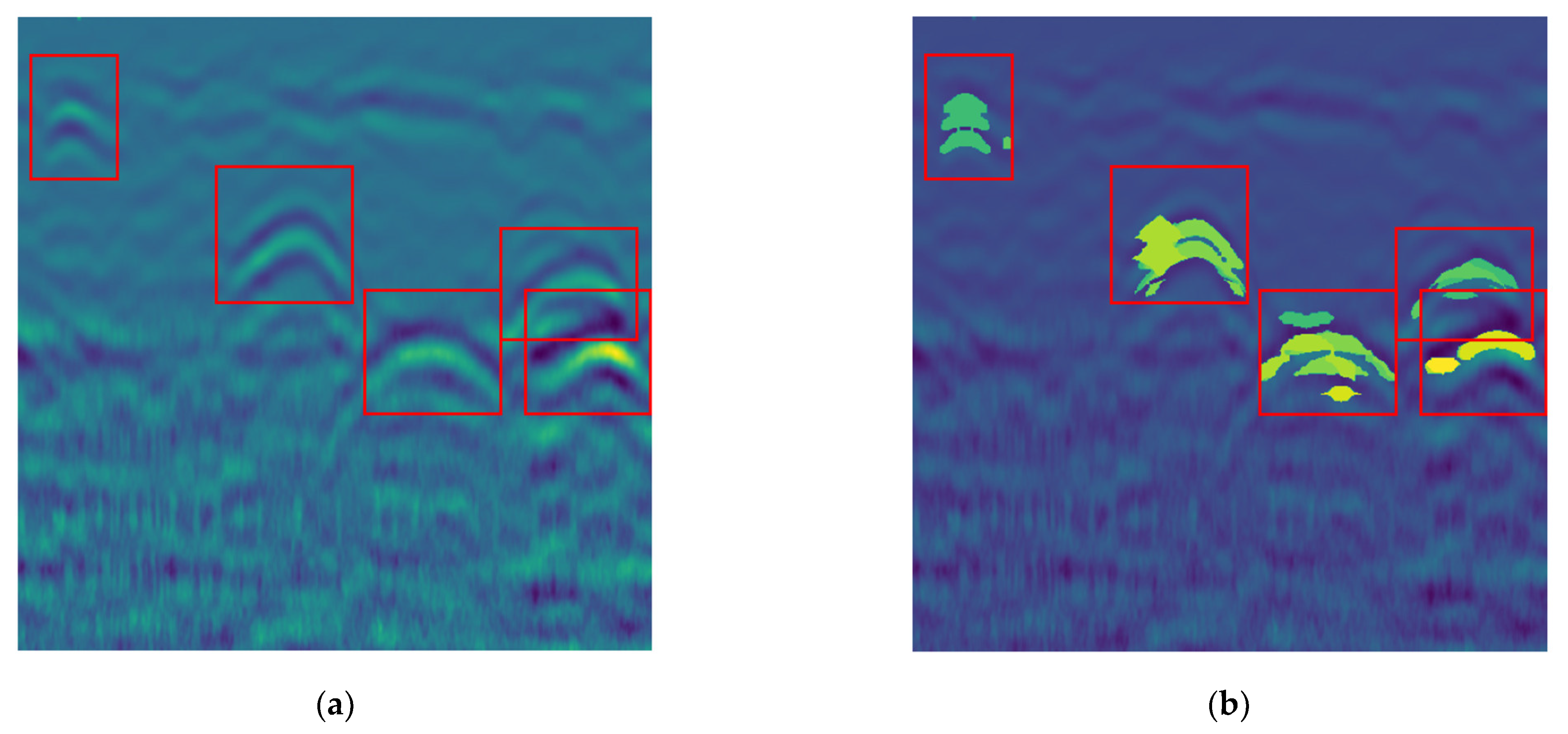
As for the on-site data, there is often much noise appearing in the B-Scan image. That would not only cause much redundant calculation but also influence the area extraction. Therefore, the stage for the on-site B-Scan image segmentation was applied after the hyperbola region detection. Figure 18 shows the extraction including top area and connected symmetrical area based on the proposal region obtained from Faster RCNN. From the output, the hyperbola region was extracted in each proposal box. At the same time, there are considerable interference areas due to the complexity of the underground environment showing no opening shape. Thus, the down opening check is necessary for the hyperbola fitting phase to filter these areas.

4.3. Analysis of Hyperbola Fitting and Information Estimation

After the hyperbola extraction, the top area and its connected symmetrical area was obtained and matched. In each top area, a key point $\left(x_0,t_0\right)$ which was helpful to simplify the geometric model equation and transform the coordinate system as important prior knowledge was searched. For each connected symmetrical area, the point set was too large to do a hyperbola fitting. In this study, the percentage point method was adopted to filter the set and gained some points as fitting point set for hyperbola fitting. Coordinate transformation and line detection with Hough transform were performed twice on the key point of the fitting point set. Thus, the radius and position of the root could also be estimated from the corresponding hyperbola equation. The relative error (RE) which was calculated by Equation (18) was adopted to evaluate the accuracy of the estimation. In the equation, $V_{real}$ is the true value and the $V_{pro}$ is the estimated value.

$$RE=\frac{V_{real}-V_{pro}}{V_{real}}$$

(18)

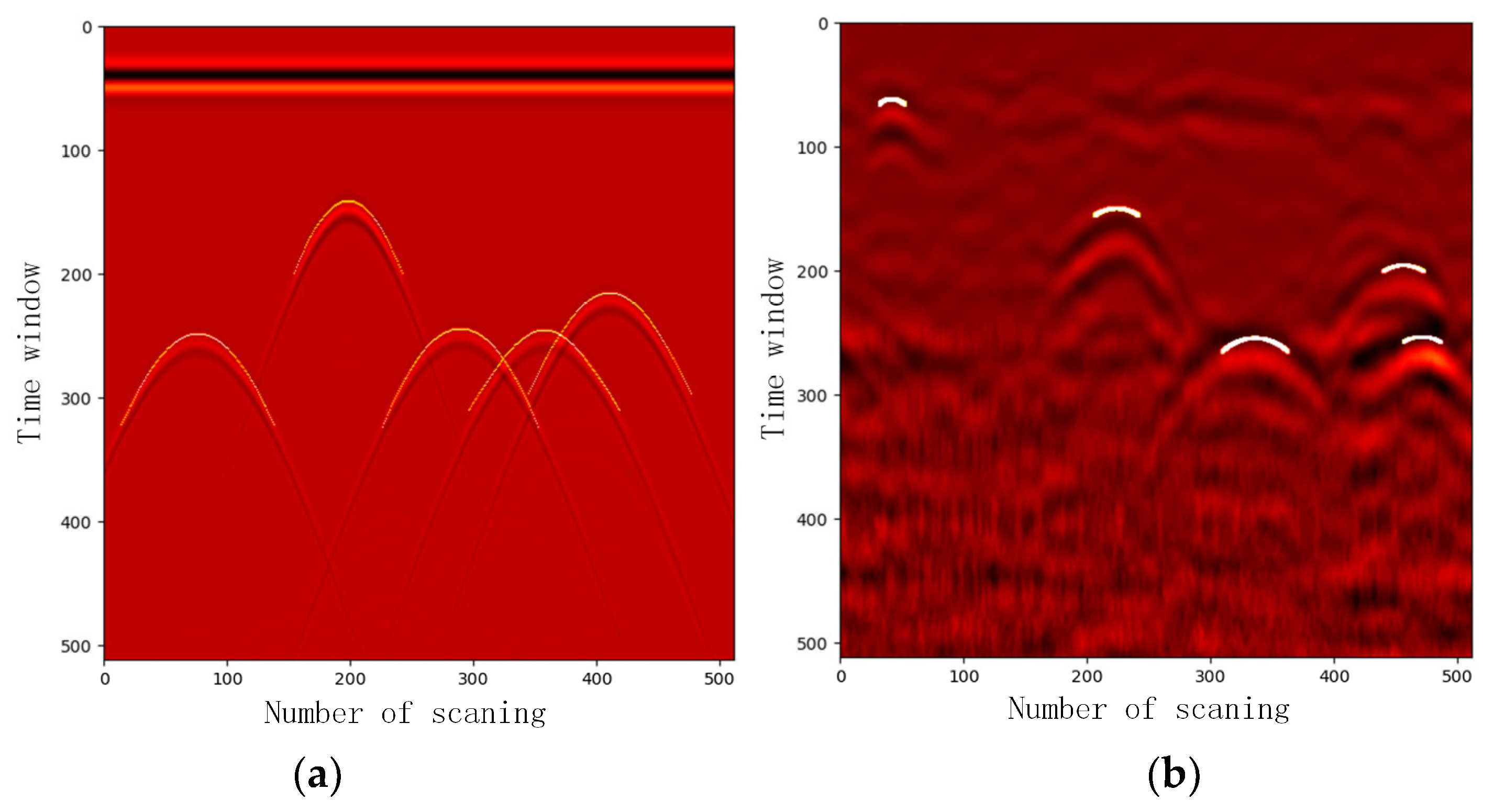
In this stage, several B-Scan images from the simulation data and on-site data were used to verify the accuracy of the hyperbola fitting. Figure 19 shows the results of the hyperbola fitting after two times coordinate transformation and line detection. Figure 19a shows a simulation B-Scan image with five cylinders of random location. In this experiment, the left two relatively independent hyperbolas were fine fitted and the right three overlapping hyperbolas could also be separated and fitted respectively. The result shows varying degrees of fitting each hyperbola of the right three owing to the use of the symmetry of the hyperbola to segment. In Figure 19b, five hyperbolas were found in the on-site B-Scan image from the field experimental data.

As for estimating the radius and location of the root from the B-Scan image, two simulated experiments and one controlled experiment were designed to verify the accuracy of our estimation method. In

Table 2. Radius and location estimation of the single root.

	Radius (m)			Depth (m)			Offsets (m)
No.	Real	Pro	RE	Real	Pro	RE	Real	Pro	RE
1	0.015	0.019	26%	0.265	0.266	0.4%	0.60	0.595	0.8%
2	0.025	0.027	12%	0.255	0.225	11.0%	0.60	0.60	0%
3	0.035	0.029	17%	0.245	0.232	5.3%	0.60	0.590	1.6%
4	0.10	0.103	3%	0.38	0.377	0.8%	0.60	0.60	0%
5	0.15	0.134	10%	0.33	0.33	1%	0.60	0.595	0.8%
6	0.20	0.189	5.5%	0.28	0.29	3.6%	0.60	0.595	0.8%

, there is one simulated experiment that includes six geometric models, with each model only including one root. In this test, these cylinders have the same center position but different radius. In the results, the bias of the estimation for the horizontal offset is less than 0.01 m and the RE is less than 1.6%. As for the depth estimation, the RE of five tests is less than 10% and only one test is 11%. The bias of these calculation results is less than 0.03 m. In the radius estimation, there is a gap in the first three and last three. The average RE is about 18% for the first three tests at the centimeter-level root and 6% for the rest at the decimeter level. In the other simulated experiment, there is one B-Scan image including three cylinders with the same radius and different depth as shown in

Table 3. Radius and location estimation of the multi roots.

	Radius (m)			Depth (m)			Offsets (m)
No.	Real	Pro	RE	Real	Pro	RE	Real	Pro	RE
1	0.015	0.024	60%	0.38	0.353	7.1%	0.6	0.595	0.8%
2	0.015	0.0125	16%	0.28	0.305	6.6%	1.2	1.345	12%
3	0.015	0.0131	13%	0.18	0.20	11.1%	1.8	2.095	14%

. The average RE of the horizontal offset is about 10% and the depth is 8%. The bias for the depth calculation is less than 0.03 m. As for the radius estimation, the RE of the last two tests is about 15% but the first one is 60%. The bias of these estimations is less than 0.01 m.

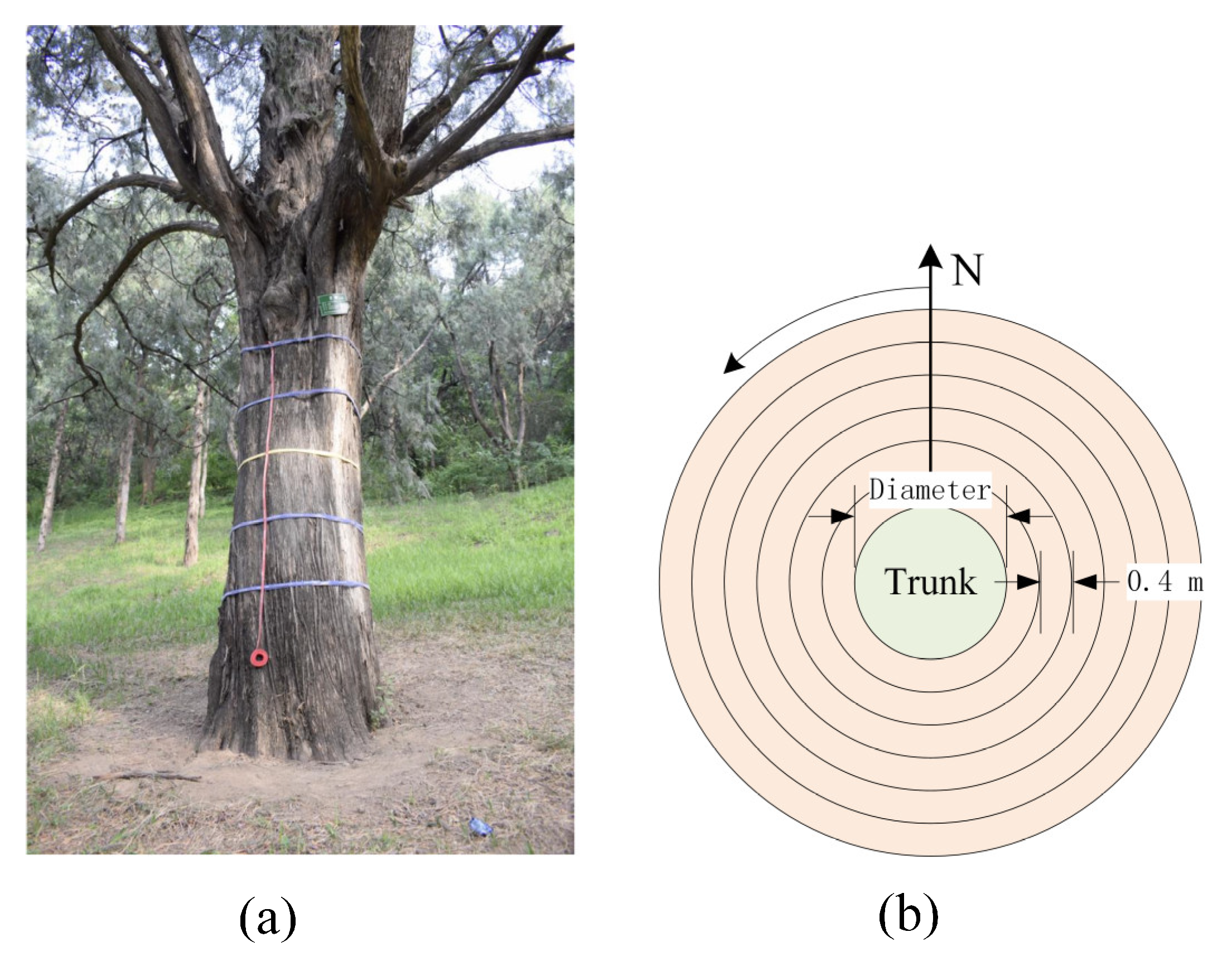
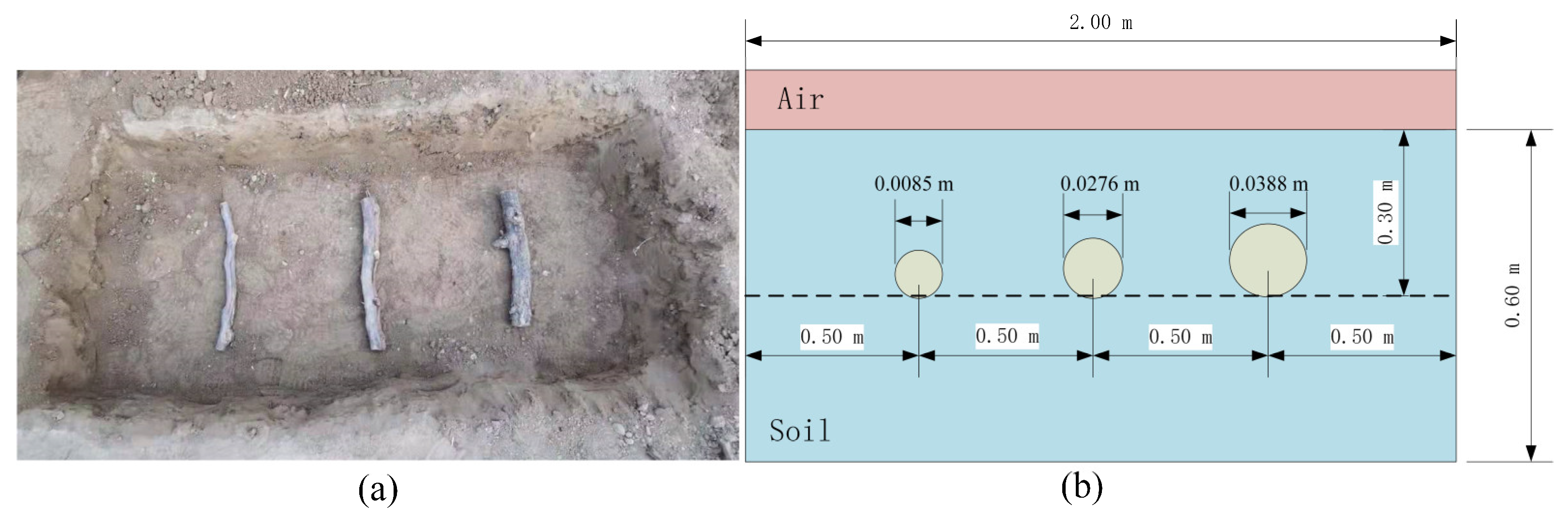
In the controlled experiment, there were three roots with different radius buried in the same depth shown in Figure 13.

Table 4. Radius and location estimation of the root in the controlled experiment.

	Radius (m)			Depth (m)			Offsets (m)
No.	Real	Pro	RE	Real	Pro	RE	Real	Pro	RE
1	0.00844	0.0082	3%	0.30	0.276	8%	0.60	0.675	12.5%
2	0.0276	0.04	45%	0.30	0.269	10.3%	1.10	1.245	13.1%
3	0.03875	−0.26	-	0.30	0.352	17.3%	1.60	1.78	11.3%

shows the results of the radius and position estimation. The average RE of the horizontal offset is about 12% and the depth is 12%. In the radius calculation, the RE of the first root is about 3%. Although the RE of the second is 45%, the bias is less than 0.013 m. As for the third root, the estimation is less than zero.

From the estimated results of the radius and position, there is an obvious gap in the relative error with different radius. The error is lower for coarse root than fine root in the simulated experiments. In this study, the size of the B-Scan image was $\left(H,W\right)$. The first element was the number of sampling points in each detection point and the second was the number of the detection points. In the scanning direction, the number of the sampling point was 512 and the distance between the two adjacent detection points was 5 mm. In the detecting direction, the depth difference between the two adjacent sampling points was calculated from Equation (19).

$$d=\frac{T}{512}\times \frac{c}{\sqrt{ϵ}}$$

(19)

$T$ is the time window, $c$ is the velocity of light, and $\epsilon$ is the relative permittivity of the soil. In our simulated experiment, the time window was 15 ns and the relative permittivity was 6. So, the sampling interval in the detecting direction was about 9 mm. If the time window was longer, the sampling interval was bigger in the same number of sampling points. Theoretically, as the number of samples increases, the image becomes finer and the signal distortion becomes smaller, but the memory occupied by the data would increase. It has been proved that the number of sampling points has a great influence on the radar image. Owing to the many small underground abnormalities, too many sampling points will appear too much noise, too few will lose useful information in the B-Scan image [66]. That caused a larger influence on fine roots than coarse roots. In the field experiment, owing to the soil anisotropy and natural stratification, moisture content, and material content usually showed differences at different depths and directions. Therefore, that was the reason for the complexity of soil distribution and further caused the relative permittivity is diversity in the soil. Owing to this, the radius and position estimations of the roots in the controlled experiment were badly affected.

In summary, there were some limitations in our method after analysis. From the result of the hyperbola region proposition, there was some missed detection in the hyperbola dense area. For some on-site data, the low confidence of the hyperbola proposal region was caused by the underground complex environment. At the same time, the symmetry test, coordinate transformation, and hyperbola detection were mainly dependent on the key point which was obtained from the multi-directional gradient graphs. This might be influenced by some noise. In addition, the resolution of the B-Scan image could also affect the accuracy of the estimation for the related information like the radius and depth of the root.

5. Conclusions

In this study, we focus on the characteristics in detection direction and scanning direction as well as the symmetry of hyperbola. A novel method of hyperbola detection based on the vertex of hyperbola for tree root detection in GPR B-Scan image was proposed. The conclusions are as follows:

• The proposed method of hyperbola recognition considering the characteristics of two directions and the symmetry of the hyperbola showed a significant effect in tree root detection from the results of hyperbola recognition as well as the estimation for the radius and position of the root.
• The characteristics both in detection direction and scanning direction were captured by the image gradient. The peak and tail of the hyperbola were obtained from the longitudinal and transverse gradient graphs.
• The multiple intersecting hyperbolas were separated with the symmetry of the hyperbola, which could reduce the influence of the rough boundary and hole inside.
• The parabola and hyperbola equations were simplified for down opening check and hyperbola fitting by coordinate transformation based on the peak area. The error caused by discretization of the parameter domain was reduced by replacing Cartesian coordinates with polar coordinates.

In the natural environment, the root is usually similar and its orientation is often unknown before digging. The detection method adopted in this paper could not guarantee vertical intersection with all roots. Guo et al. [67], Liu et al. [68], and Wang et al. [69] verified the influence of the root orientation on both A-Scan signal and B-Scan image. The root orientation was defined as horizontal angle and vertical angle. Therefore, the impact of the root orientation makes the geometric model more complex. Guo et al. [12] summarized the characteristics of root detection using GPR with different frequency antenna in terms of detection depth and GPR resolution. In our study, the frequency of the antenna is 900 MHz. Owing to the antenna frequency, the detection depth is about 1 m and the GPR resolution is about 2 cm in the sand. Some processing to reduce noise including filter, dilation, erosion, and threshold segmentation would bring some effect to the symmetry of the hyperbola. The factors influencing the symmetry of hyperbolic curves will be studied in the future.

Due to the different relative permittivity between the soil and the root, the root was detected with GPR. The water content is one of the important factors affecting the relative dielectric constant of the medium [12]. In this study [70], the pipes which contained water, a 1:1 ratio of water and air, air, and salt water (22 mg cm⁻³ iodized sea salt) were detected in the designed controlled experiments. A small difference in relative dielectric permittivity between moist soil and root affected root detection. In the actual test, the effect of root environment on the hyperbola was much smaller than that of root orientation. In the future, based on the root detection method in this paper, further research will be conducted for the detection of root with different orientation and different moisture contents.

In real detection, the root detection result could be influenced by the complexity of soil distribution and the accuracy of GPR. In the future, we will focus on more accurate object detection algorithms with stronger anti-interference and more accurate identification of hyperbola and estimation for the related information. High precision root detection could provide data support for the restoration and research of three dimensional root structure.