Curvature of Logs—Development of and Comparison between Different Calculation Approaches

Abstract

In the field of electronic roundwood measurement, 3D-laser systems are becoming more and more important for the determination of log volume and quality. Especially the outer shape of the logs is of particular importance for the yield and should therefore be described in as much detail as possible. This study focuses on the parameter curvature and compares five different approaches to quantify the sweep of logs based on high-resolution 360°-scans of 269 debarked logs of the species spruce, oak and pine. We observed strong differences between the approaches, including the two variants that are currently approved in German sawmills. Due to our findings, we suggest the introduction of a method that is based on a calculated centerline through the log instead of considering the outer log contour for future German log grading.

1. Introduction

Over the past several years, annually, on average, 30–40 million cubic meters roundwood have been cut in German sawmills [1]. For the detection of the external shape of the logs, electronic measurement systems are becoming more and more important and are already used as a basis in the majority of the billed soft wood. The use of modern 3D-laser measurement systems not only allows the calculation of the billing-relevant volume, but also the automatic determination of quality parameters such as curvature, ovality and taper is possible [2].

Since approximately one third of hardwood saw logs show a significant amount of sweep especially the curvature value is of particular importance for the quality assessment of roundwood. In German forest practice, curvature is defined as the “deviation of the longitudinal axis of the round timber from the straight line [...]” [3]. Beside genetic reasons [4,5], the causes of crookedness of trees are often browsing, one-sided incidence of light, one-sided snow and wind loads and ground movements on slopes [6]. In terms of wood technology, this can result in eccentricity, a non-parallel fiber course and increased occurrence of reaction timber [7,8]. Moreover, for the sawmill industry, the reason for an undervaluation of crooked logs is due to the potentially lower yield [9,10,11] and, especially in fast running softwood mills, a lower cutting speed in the process [8].

Even if most sawmills use internal algorithms for the maximization of the value of the products during the sawing process [12], an objective assessment for quality parameters for both market partners (forest owners and sawmills) is required. For the calculation of curvature, so far two different basic approaches can be observed (Figure 1). The first variant is based on the outer shape of the logs and calculates a bow height as the maximum distance between the contour of the logs and a reference line outside the trunk. The second variant uses a centerline (e.g., calculated as the center of mass at each virtual slice) through the log and calculates the maximum distance between this line and a straight line between the end points of the centerline. The final value for curvature is then determined through a division of the bow height by the length of the log (e.g., Germany: Rahmenvereinbarung für den Rundholzhandel in Deutschland [3]) or the division by the diameter in the middle of the log (e.g., Austria: ÖNORM L 1021:2015 08 01).

In Germany, the DFWR (Deutscher Forstwirtschaftsrat)/VDS (Verband der Sägeindustrie) framework agreement (Version 14 January 2005) has been regulating the measurement of logs in sawmills in private law since 2005. According to this agreement (Rahmenvereinbarung für die Werksvermessung in Deutschland RV WV), two permissible process variants (contour method and a segment approach based on the centerline method) are currently approved to determine the curvature of logs, until a decision for one of the methods can be reached based on sufficient practical experience. Even if the segment approach has never been implemented in a measurement unit, both methods are still possible for new registrations of measuring systems according to RV WV; a comprehensive assessment of the two variants (and possibly additional methods) has not yet been carried out.

The aim of this paper is to close this knowledge gap by investigating different calculation methods, to submit suggestions for improvements and, moreover, to develop alternative methods. Both the existing procedures with their modifications and the newly developed approaches are therefore translated into algorithms and tested using measurements of real logs. In addition, the influence of the offsets of the reference line and the smoothing method for the center line are discussed as part of a sensitivity analysis.

2. Materials and Methods

2.1. Sampling Logs

For the study, we used a total of 269 debarked logs (nominal length of 5 m) of the tree species Quercus robur L. (50 pieces, oak), Picea abies L. (87 pieces, spruce) and Pinus sylvestris L. (132 pieces, pine) (

Table 1. Summary of the observed logs (data from manual measurement).

Species	Number of Logs	Mean Center Diameter [cm] (sd)	Mean Physical Log Volume [m3] (sd)
spruce	87	23.7 (3.8)	0.17 (0.06)
oak	50	20.9 (3.1)	0.14 (0.04)
pine	132	30.0 (4.7)	0.29 (0.09)

). To get crooked material, the spruce logs were collected over a period of several weeks on the log yard of a South-German sawmill during usual operation in autumn 2020. The pines originate from different stocks located in the south of Baden-Wuerttemberg; the oaks were taken from a stock in southern Rhineland-Palatinate. Heavily damaged individuals as well as logs shorter than 5.05 m were excluded from the analysis.

2.2. Log Measurements

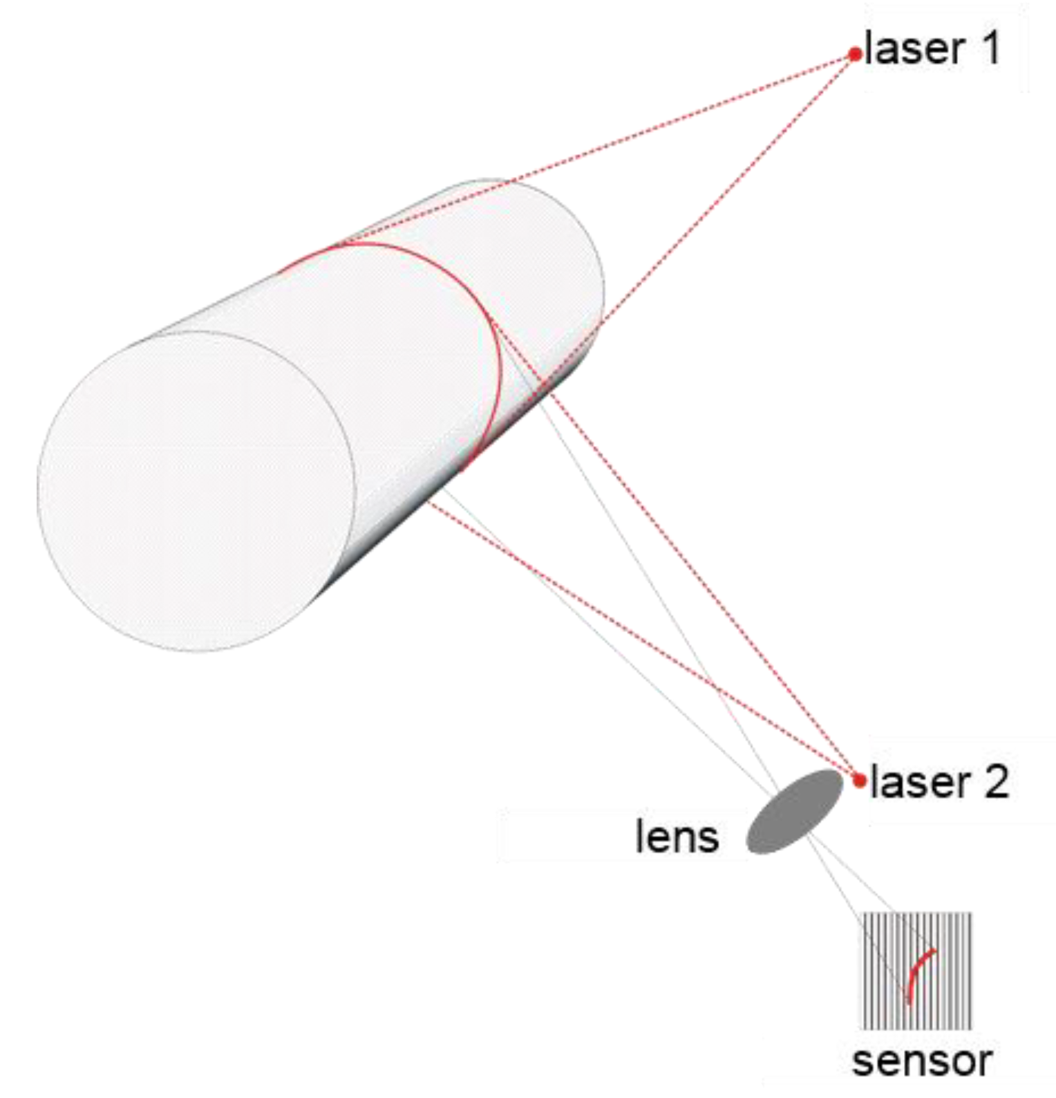
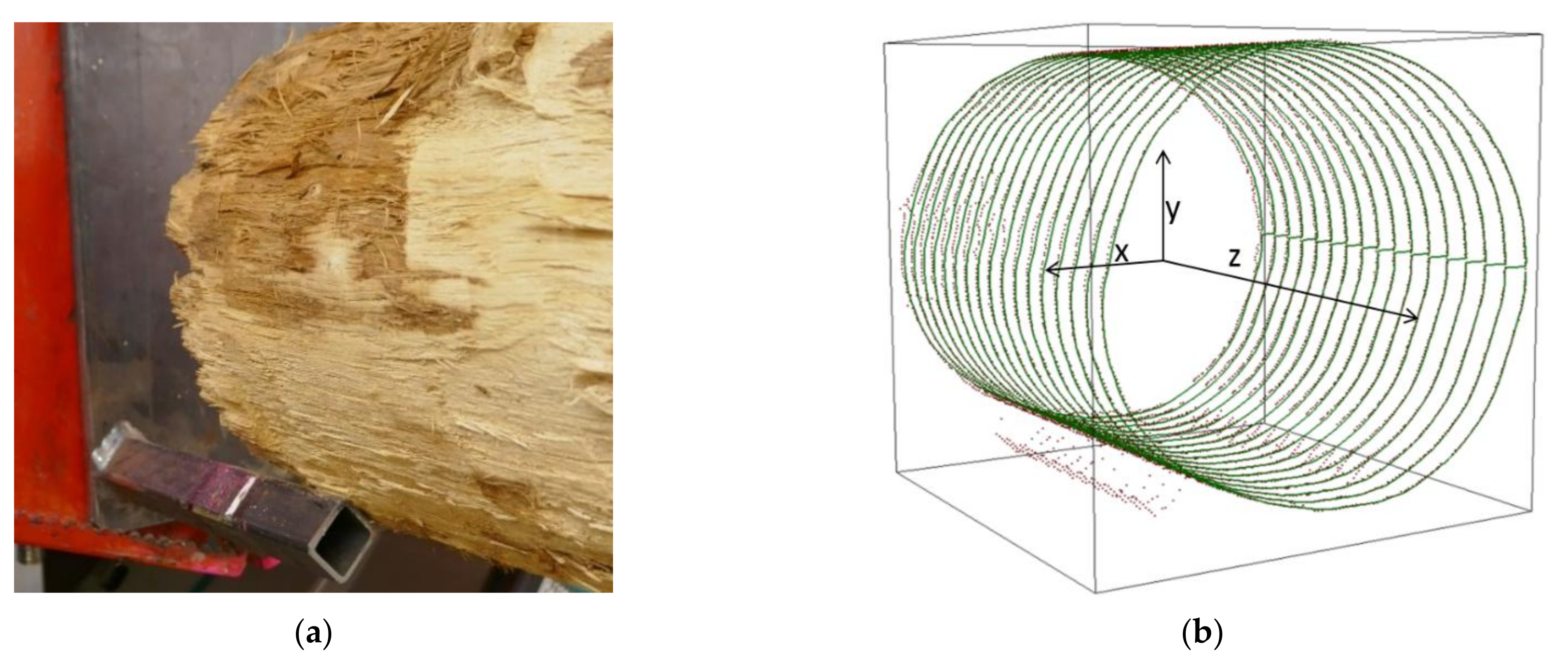
Modern measuring systems for recording log contours are currently usually based on laser triangulation [13]: a laser beam is reflected by the surface of the respective object and projected onto a light-sensitive sensor through a lens. If the geometry of the entire measuring system and the properties of the lens are known and several laser sources and sensors are used, the external shape of the object can be derived from the position of the imaging points on the receiver (Figure 2).

For our measurements, we used a DiShape system (Microtec Srl, Brixen, Italy), which is permanently installed at the Forest Research Institute of Baden-Wuerttemberg in Freiburg. The system delivers 3D-point data (360 points per slice) at an interval of about 5 mm in the longitudinal direction, so that a 5 m-log is described by approximately 360,000 data points (1000 slices).

In addition to the electronic measurement, all spruce and pine logs that visually showed a curvature (179 of 219 logs) were measured manually according to the RVR (Rahmenvereinbarung für den Rohholzhandel in Deutschland). The only difference was the offset of the reference line: in order to be able to compare the results of the manual measurement with the curvature values of the contour method according to RV WV, an offset of 0.5 m (instead of 1.0 m according to RVR) towards the middle of the log was made at the butt end. The manual measurement was carried out as a two-man procedure, the parameters, physical length [m], type length [m], physical center diameter after cross-clipping [cm], bow height [mm], and position of the bow height measured as the distance to the logs’ butt end were recorded.

2.3. Preprocessing of Data

From the software point data were exported as .txt files (ASCII-format). Since the geometry of the measuring system at the FVA (due to the supports that are needed to fix the logs during the measurement process) results in inaccuracies at the last eight centimeters on either side, the data had to be corrected in these areas. The correction was made by linear interpolation of the mean coordinates of the log slices immediately before (5 cm interval) the supports begin (Figure 3). Since these areas are very small (<1.6% of the log length), an adjustment via a taper value was considered unnecessary as these parts of the log do not have a relevant impact on the results.

In order to exclude outliers that come from log defects such as bark chips, bad debranching quality or ripped out parts of the xylem, we applied an iterative filter at each slice of the logs. For each point, we calculated the distance (dis_i) to the center of mass of the slice. If the absolute of this value minus the mean distance from the two neighboring points (dis_{i−1, i+1}) was higher than 10%, the point was classified as implausible and replaced by the mean value of the four neighboring points. We defined the 10% threshold based on visual assessment on randomly chosen slices of different logs. The number of iterations was set to three, since this value turned out to be a good compromise between eliminating outliers and over-smoothing the real surface.

2.4. Development of Algorithms

All in all, five algorithms were assessed in this analysis and are detailed below:

• contour: Variant 1 according RV WV;
• segment: Variant 2 according to RV WV;
• centerline: Method of “center of mass”;
• centerline ellipse: Method “ellipse-fit”;
• differential: Based on the mathematical definition of curvature.

All procedures were programmed in the open source software environment R (R Version 3.6.1) using the packages rgl (0.110.54, Adler, D. and Murdoch, D.), plot3D (1.3, Soetaert, K.) and Conicfit (1.0.4, Gama, J. and Chernov, N.) for implementation.

2.4.1. Contour Method According to RV WV

Based on the filtered data, 36 reference lines (see Figure 1) were created on the virtual log. Since after increasing the number of reference lines higher than 36 (and thus having an angle of 10° between them) the curvature value did not significantly change anymore, we used this setting in our analysis. The suspension points of the lines are determined as follows: There is an optional offset on both the butt end and the top end of the log. Since there is usually no measuring plane at the Z-offset (in the axial direction), the suspension point is formed from the mean value of the Z-values recorded in a 10 cm interval to the left and right of this point. The X- and Y-coordinates of the suspension point also result from averaging the respective values in the 10 cm interval. From the so formed two suspension points (X, Y, Z) of each reference line, an equation is defined in three-dimensional space, according to which the coordinates of the line are calculated for all Z-values of the measured planes. For each of the defined lines, a bow height is determined as the maximum over all measured distances at each Z-coordinate (only if the reference line is outside the log contour, the “negative” bow heights are not included in the analysis). The highest value of the bow heights of all reference lines is saved as the final value that is included in the calculation of the curvature according to the formula

$$cur\left[\frac{\mathrm{cm}}{\mathrm{mm}}\right]=\frac{\frac{B\left[\mathrm{mm}\right]}{10}}{L_{\mathrm{N}}\left[\mathrm{m}\right]-O\left[\mathrm{m}\right]},$$

(1)

where B represents the maximal bow height, L_N the nominal length of the log and O the offsets of the reference line (resp. the sum of offsets if applied on both butt and top end).

2.4.2. Interpretation of the Segment Method According to RV WV

Based on the ideas of Wilwerding [14], who developed a procedure to calculate the curvature of a log as the sum of more than one bow height, we developed an algorithm to implement the substance of this idea. Since, in the current version of the RV WV, a couple of calculation steps remain unclear, we had to make some assumptions and amendments: Starting from the middle of the observed log, N measuring points are localized in 50 cm steps in both directions (Figure 4). Since there is usually no measuring plane at the Z-values determined in this way, the slice with the smallest distance to this theoretical value (maximum 3 mm for the Microtec system) is used. The centroids of each slice are calculated by averaging all X- and Y-coordinates of the corresponding Z-value and joined to a center line through the log. Analogous to the determination of the reference line in the aforementioned contour method, an offset on both sides of the log can be applied. Since this Z-offset usually does not represent a measuring plane, the suspension point is calculated from the mean value of the Z-values that are in a 10 cm interval to the left and right of this point. The center of mass is now calculated for each slice in this area, the suspension point of the reference line results from the mean value of the centers in the defined segment. N bow heights are now determined by calculating the shortest distance between both lines. The calculation of the “exceeding curvature” (cur.exc) at each of the measuring points x takes place by subtracting a diameter-dependent acceptable curvature (cur.acc) from the determined bow height B_x according to

$$cur.ex{c}_x\left[\mathrm{mm}\right]=B_x\left[\mathrm{mm}\right]-\frac{d_{x1}\left[\mathrm{mm}\right]+d_{x2}\left[\mathrm{mm}\right]}{2}cur.acc\left[\%\right],$$

(2)

where d_x1 and d_x2 represent diameters that are measured in two defined planes, that are perpendicular to each other. The final value cur then results conforming to

$$cur\left[\%\right]=100\frac{\frac{{{\displaystyle \sum }}_{x=1}^{N}cur.ex{c}_x\left[\mathrm{mm}\right]}{n}}{\frac{d_{\mathrm{m}.1}\left[\mathrm{mm}\right]+d_{\mathrm{m}.2}\left[\mathrm{mm}\right]}{2}},$$

(3)

where d_m.1 and d_m.2 represent two diameters that are measured in the middle of the log (again in two planes with an angle of 90°).

2.4.3. Centerline Method Based on the Center of Mass

If not the outer contour but the course of a center line through the log is used to calculate one maximum bow height, there are several calculation options. One variant is to determine the geometric centers of mass of each slice and then connect these points to a line through the log (see segment method). In this method, however, the log is not divided into segments, but, analogous to the contour method, only the maximum bow height is used to calculate the curvature value. As in the segment method, the reference line is formed on the basis of previously defined offsets; the center line is also calculated analogously. In order to further reduce the influence of surface defects, the center line is afterwards smoothed using the moving average method with a tunable bandwidth (in our analysis we tested 5, 10, 15 and 20 cm).

2.4.4. Center Line Method Based on Ellipse Fits

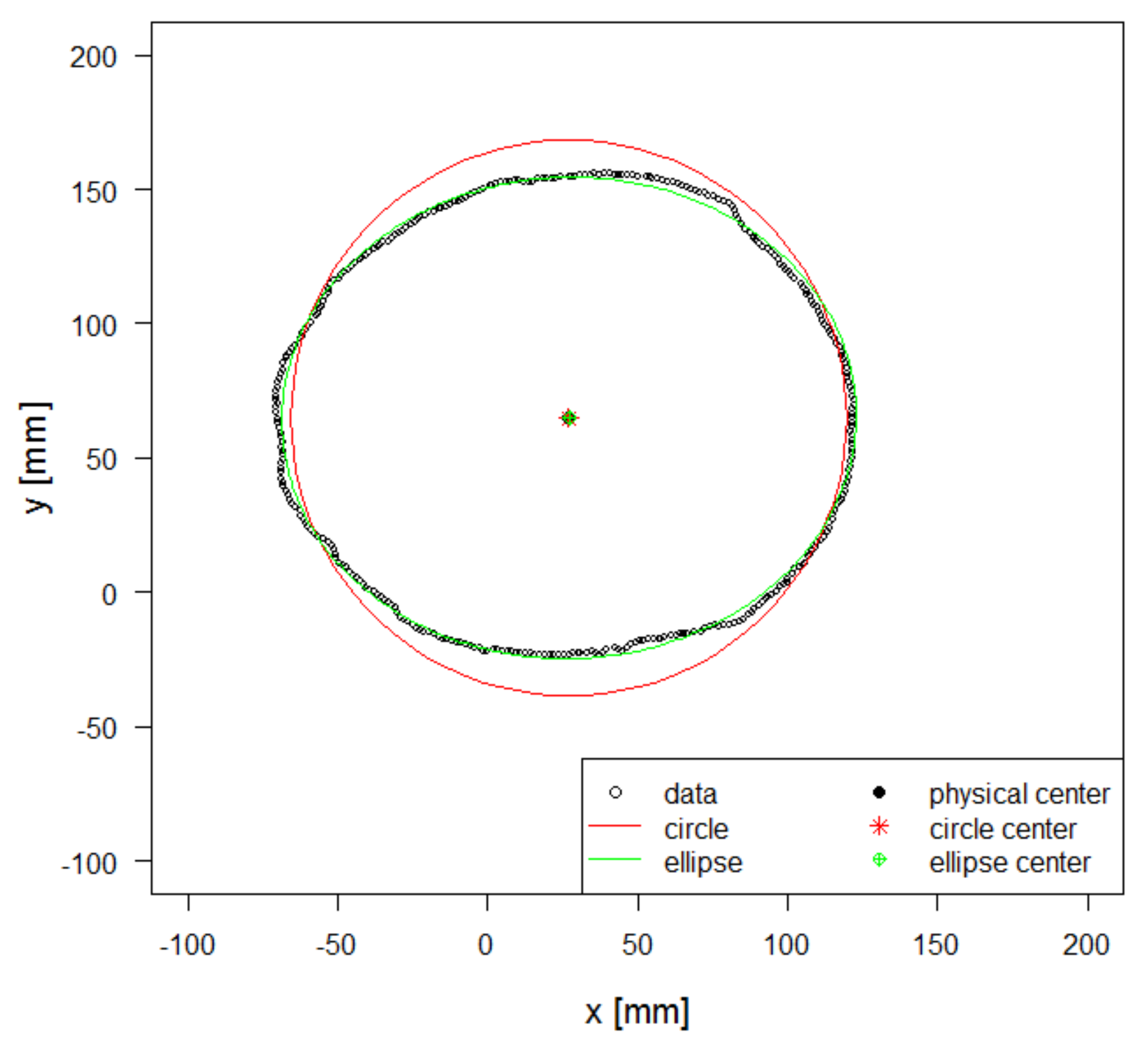
Another way of calculating a center line through the trunk is to approximate the individual slices using ellipses or circles and to connect their center points. Starting from the 360 points of a slice, both an approximate circle and an ellipse can be fitted using a least-squares approach. (Figure 5). The calculations of the reference line and the smoothing of the center line are carried out in the same way as in the center line method based on the centers of mass.

2.4.5. Differential Approach

Mathematical curvature is defined as the local deviation of a curve from a straight line. Thus, the difference from the original issue of finding the log’s curvature is that the definition of mathematical curvature only yields a local quantity in each point of a curve and not a log-wide curvature. Among the several possible approaches to approximate the mathematical curvature [15,16,17], we chose a relatively simple and straightforward one. The basic idea is to approximate the fundamental course of the trunk by the course of the centers of mass of each slice and then calculate the average mathematical curvature of this curve in the centers of mass.

First, to avoid an influence of different log diameters on the log curvature, the diameter of each log is normalized, i.e., the coordinates of each point are divided by the average distance of all points to the centers of mass of the slice they belong to. The centers of mass of these normalized logs are then regarded as points of a regular and sufficiently smooth curve f, whose curvature κ in the point (x₀, y₀, z₀) can be calculated by [18]

$$\kappa \left(x_0,y_0,z_0\right)=\frac{\left|\right|f^{\prime }\left(x_0,y_0,z_0\right)\times f^{″}\left(x_0,y_0,z_0\right)\left|\right|}{\left|\right|f^{\prime }{\left(x_0,y_0,z_0\right)\left|\right|}^3}=\frac{\sqrt{\left|\right|f^{\prime }{\left(x_0,y_0,z_0\right)\left|\right|}^2\left|\right|f^{″}{\left(x_0,y_0,z_0\right)\left|\right|}^2-{\left(f^{\prime }\left(x_0,y_0,z_0\right)·f^{″}\left(x_0,y_0,z_0\right)\right)}^2}}{\left|\right|f^{\prime }{\left(x_0,y_0,z_0\right)\left|\right|}^3}$$

(4)

with $f^{\prime }$ and $f^{″}$ as the first and second derivative, $\times$ the cross-product, $\left|\right|.\left|\right|$ the Euclidean norm, and $·$ the Euclidean dot product.

As the mathematical curvature is more heavily effected by local deviations of the centers of mass than the previous methods, the curve defined by the centers of mass is heavily smoothed by a median and averaging filter (500 mm interval), in order to extract the underlying course of the log, before calculating the curvatures in the centers of mass. To calculate the curvature in the centers of mass of each slice with Equation (4), the calculation of derivatives of the curve f in these points is required. We used the forward difference quotient for the first derivative and a central difference quotient for the second derivative to approximate the derivatives [19], i.e., the derivative in the center of mass x_i of the i-th slice is defined by

$$\begin{gathered} f^{\prime }\left(x_i\right)\approx \frac{f\left(x_{i+1}\right)-f\left(x_i\right)}{x_{i+1}-x_i} \\ \mathrm{and} \\ {f}^{″}\left(x_i\right)\approx \frac{f\left(x_{i+1}\right)-2f\left(x_i\right)+f\left(x_{i-1}\right)}{{(x_{i+1}-x_i)}^2}, \end{gathered}$$

where $x_{j+k}$ is the center of mass of the (j+k)-th slice. As with the other methods, an offset on both sides of the log is useful and therefore applied. This also reduces or even eliminates the issues with calculating the smoothing filters or the derivatives at the log ends. Since we are not interested in the local curvature in each point, but a global quantity, we finally define the log curvature as the average of the approximations of the mathematical curvatures computed in the centers of mass of each slice.

2.5. Validation and Comparison of Methods

For the manual measurement, the contour method and both of the center line approaches, the target variable is a curvature value according to Equation (1). These methods can thus be compared directly. In contrast, the segment method and the differential method deliver data that cannot directly be related with these findings (curvature [%] for the segment method calculated by the division of a mean bow height by the diameter of the log; a curvature value in mm⁻¹ for the differential approach). To nevertheless be able to compare all approaches, we plotted each method against the manual measurement and calculated the correlation between each approach using Spearman’s ρ for non-normal distributed data [20].

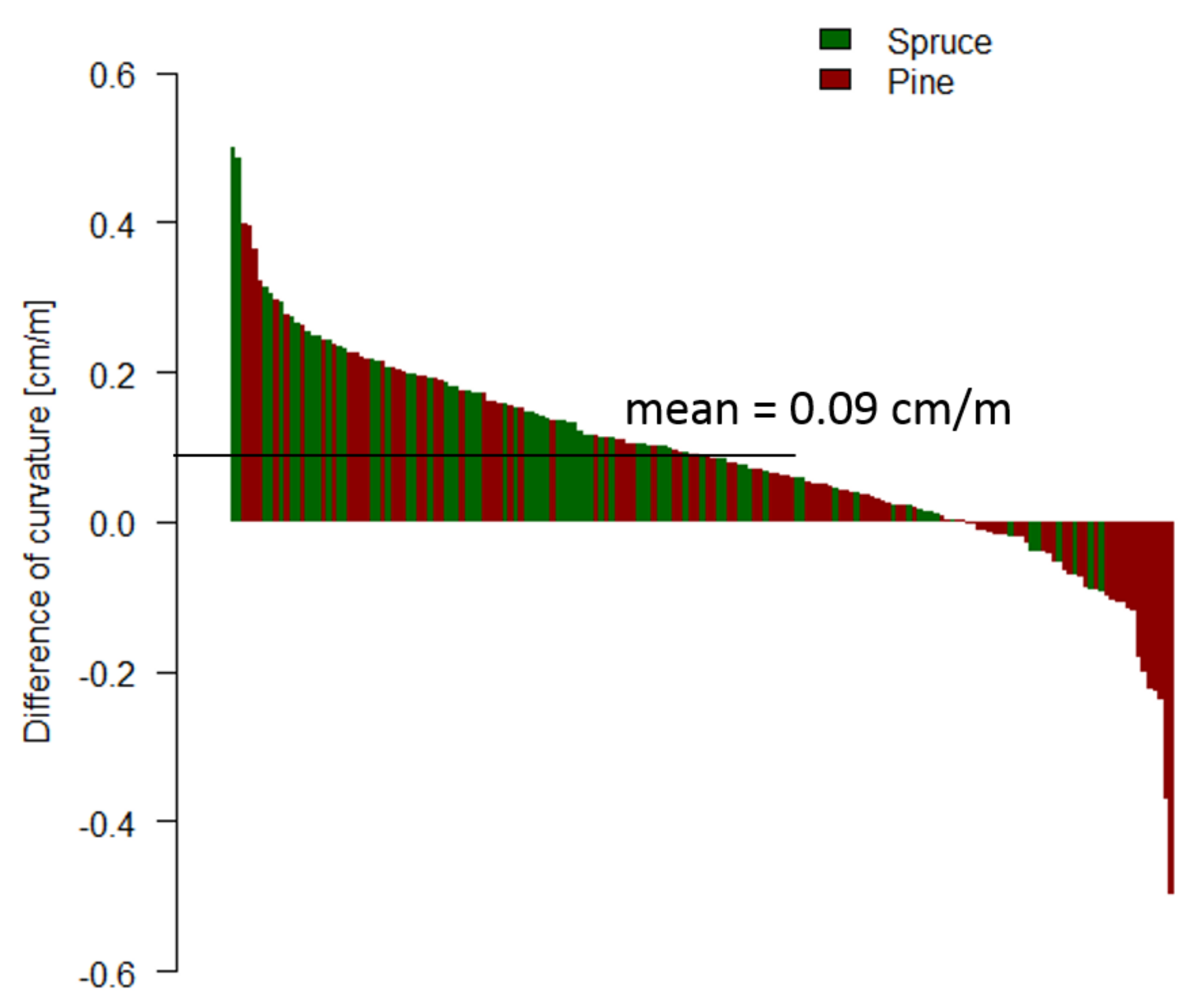
Since the current algorithms for the calculation of the curvature according to the contour approach in the sawmills were not accessible, our implementation of it was validated by using the error ranges from the certification process of the RV WV [21]:

• maximum mean deviation 0.1 cm/m between manual measurement and contour algorithm
• >0.3 cm/m deviation between manual measurement and contour algorithm in less than 10% of the logs.

3. Results

3.1. Validation of Contour Approach

The contour algorithm exposed substantially stronger curvature values than the manual measurement (Appendix A Figure A1). In addition, 7.8% of the logs show a difference >0.3 cm/m, the mean difference is 0.09 cm/m. The variations are higher for spruce (mean 0.13) than for pine (mean 0.06) but for both, the algorithms more often shows higher values than the manual measurement (pine 72.6%, spruce 90.4%).

3.2. Comparison of All Approaches

For the comparison of all approaches, we calculated curvature values using the current standards for the offsets of the RV WV (500 mm at butt end, 0 mm at top end). The centerlines were smoothed using a 10 cm interval for the moving average; the accepted curvature for the segment method was set to 0. The highest correlation between an algorithm and the manual measurement could be found for the center ellipse and the contour approach (ρ = 0.94), followed by the center mass algorithm (ρ = 0.94), the segment approach (ρ = 0.79) and the differential procedure (ρ = 0.70) (Figure 6). What is striking too is that, in all but the differential approach, the species does not seem to have a crucial impact on the relationship between two methods (visually expressed by a varied mixture of the species within the plot).

Within the algorithms, the smallest difference can be found between both center line methods (center mass and center ellipse, ρ = 1), the highest differences between the segment method and the differential approach (ρ = 0.61). Both center line methods show high correlation with the contour method (ρ = 0.97) but lower correlation with the segment method (ρ = 0.94) and the differential approach (ρ = 0.72). The contour and segment method (which are currently both permissible for new registrations of measuring systems) show a correlation of 0.90, the contour method and the differential approach a relatively low ρ of 0.70.

3.3. Comparison between Contour and Center Line Method

Since the contour method and the center mass method both result in values [cm/m] that can directly be compared with each other, we plotted the absolute differences for those two approaches (Appendix A Figure A2). For each log (across all tree species), the contour method provides higher values for the curvature (mean difference 0.22 cm/m, median 0.19 cm/m) than the centerline method, which also would result in a diverging quality classification.

3.4. Sensitivity Analysis

3.4.1. Offset of Reference Lines

To quantify the effect of the offsets of the reference lines on the butt and top end of the log, we calculated the curvature for the centerline method with six different combinations (

Table 2. Mean of curvature values according to the centerline method in cm/m for different combinations of offsets of the reference line at the butt end (B) and the top end (T) in mm for the 269 logs by species. No offset on both ends of the log (B0_T0) would result in a mean curvature of 0.79 for spruce, 1.61 for oak and 1.05 for pine.

Species	B0_T0 [cm/m]	B200_T0 [cm/m]	B500_T0 [cm/m]	B1000_T0 [cm/m]	B200_T200 [cm/m]	B500_T200 [cm/m]
spruce	0.79	0.81	0.78	0.70	0.83	0.80
oak	1.61	1.67	1.65	1.67	1.70	1.69
pine	1.05	1.07	1.04	0.98	1.09	1.07

) including the current regulation according to RV WV (butt end: 500 mm, top end: 0 mm). The lowest values for spruce (0.70) and pine (0.98) can be found for an offset of 1000 mm at the butt and 0 mm at the top end (B1000_T0); for oak, the lowest value can be found when no offset is applied (B0_T0). Within one species, the biggest effect of the different offsets can be found for spruce (15.7%), followed by pine (10.3%) and oak (5.3%).

3.4.2. Smoothing

Even if a first smoothing of data is already done through the filtering process and the calculation of the corresponding center of each slice in the centerline approach, individual outliers of the centerline can still falsify the result and therefore should be mitigated by applying a further smoothing [22]. For this reason, we also applied smoothing for the center ellipse and the segment approach. To quantify the effect of five varying intervals for the moving average smoothing of the centerline (50 to 1000 mm, Figure 7), we calculated the mean curvature by species according to the centerline approach with the offsets for the reference line of the RV WV (butt end: 500 mm, top end: 0 mm).

For each species, the curvature value is slightly reduced by increasing the interval (2nd decimal place), a significant difference of the effect of smoothing between the three species cannot be observed (

Table 3. Mean curvature values for the centerline method depending on the smoothing interval used for the calculation of the moving average divided by species. For an interval of 50 mm (C_50), the mean curvature value is 0.78 for the spruce logs, 1.68 for the oak logs and 1.05 for the pine logs.

Species	C_50 [cm/m]	C_100 [cm/m]	C_150 [cm/m]	C_200 [cm/m]
spruce	0.78	0.77	0.76	0.75
oak	1.68	1.67	1.65	1.62
pine	1.05	1.04	1.03	1.02

).

4. Discussion

Even if our algorithm for the contour method almost exceeds one of the two error rates for the certification of new measurement systems (0.09 cm/m which is only slightly below the threshold for the mean deviation), it can still be considered as a reliable interpretation of the procedure described in the RV WV. Since we only observed extreme variants of curved logs and excluded straight individuals from the validation process, we can expect smaller differences for a more representative sample of logs that are usually processed in sawmills. Moreover, our reference is not particularly accurate: deviations still can result from mistakes in manual measurement.

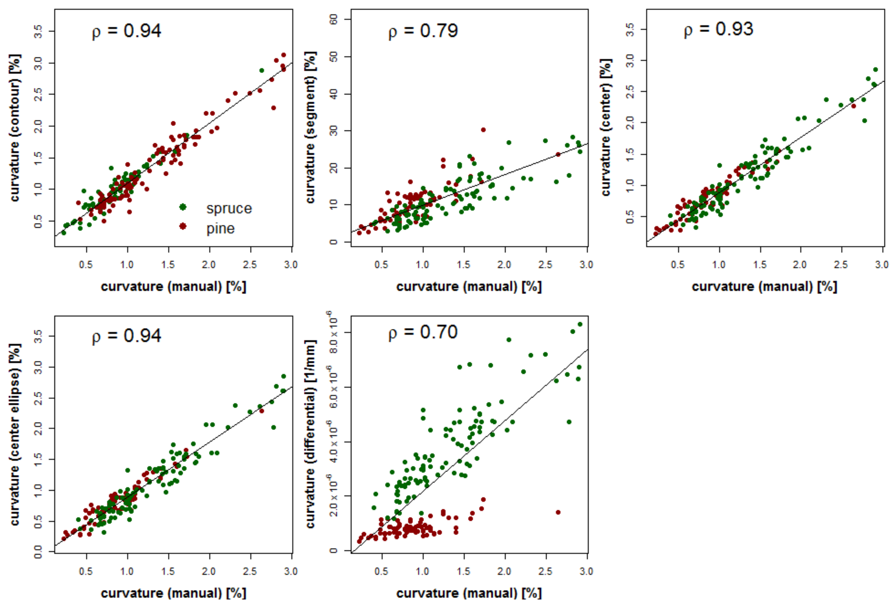
The comparison of all five approaches with the manual measurements (Figure 6) shows that different methods of the calculation of a curvature for logs can result in partly very diverse rankings according to this log quality parameter. In particular, the segment method and the new differential approach differ widely from the established contour algorithm and the centerline approaches (expressed by low values for the correlation coefficient ρ between the different methods). The fact that according to the RV WV contour and segment method are currently both permissible for the new registration of measuring systems according to RV WV, could therefore lead to different quality ratings of the same logs in German sawmills. This can neither from a theoretical nor from a practical point of view be recommended. The basic idea of the segment approach could thereby basically be target-aimed: instead of only considering one maximum value for the bow height, the course of the curvature through the whole log is regarded. Nevertheless, different types of curvature (e.g., suggested by Gjerdrum et al. (2004) [23].) still can’t be detected and would require the integration of further sweep characteristics.

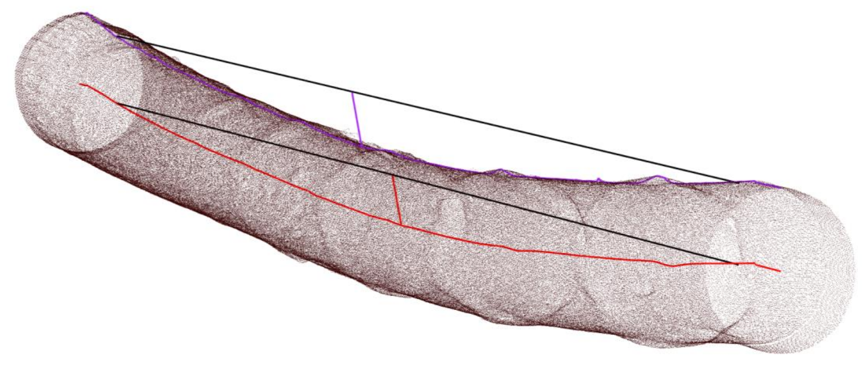
One explanation for the difference between segment and contour approach can be seen in the surface of the log: slight hollows or surface defects are directly detected through the contour approach, whereas, in the centerline methods, they are already smoothed out through the calculation of the center of mass (Figure 8). Even if this effect in the contour approach could be reduced by a stronger a priori filtering process of all data points, calculating the center is from our point of view still the better option because it is easy to implement, comprehensible and far less dependent on different filtering techniques of the measurement system manufacturers. Moreover, if one aims for an automatic deduction of a curvature type, the course of the centerline can offer promising options to predict it [2,23].

Both centerline approaches (center mass, ellipse fit) do not differ in their evaluation of curvature (ρ = 1) and basically could therefore be recommended for the calculation of a bow height, whereas the easier implementation and comprehensibility could be seen as an argument for the former. The differential approach showed by far the lowest correlation with all other approaches and the manual measurement, which can mainly be explained by the strong effect of tree species on its curvature value. This for now makes this algorithm unusable for practical uses.

The effect of the implementation of different offsets of the reference line is maximal for the observed spruce logs (difference of 0.13 cm/m i.e., 16% between B1000_T0 and B200_T200). Nevertheless, we agree with Weidenhiller and Golser [22] that an offset should be applied on both sides of the logs, since most of the damages and surface defects can be found in these areas. The effect of the different smoothing intervals is in contrast very small (maximal 0.06 cm/m i.e., 4% between 200 mm and 50 mm interval for oak). Here our findings are basically consistent with Weidenhiller and Golser [22] who found a maximum difference of 4.6 mm of bow height (=0.09 cm/m for a 5 m log) for their observed logs. Based on these findings, we would recommend offsets for the reference line of 500 mm at the butt end and 200 mm at the top end in combination with an interval of 200 mm for smoothing the centerline which would make sure that, after the offsets are applied, there is still a wide enough distance towards the log ends for applying the moving average filter.

Independent of the method of the detection of the bow height, the current curvature value according to the RV WV (contour method) and also according to RVR (manual measurement) is calculated by dividing the bow height by the length of the log. This procedure can cause two inaccuracies: On the one hand, two logs with the same curvature, one thin, one very big, result in the same value, even if the effect of the sweep is (in terms of yield) much worse for the thin than for the big log. So far in Germany, this is partly solved by diameter-specific limits (three diameter classes) for the grading of the log in the RVR.

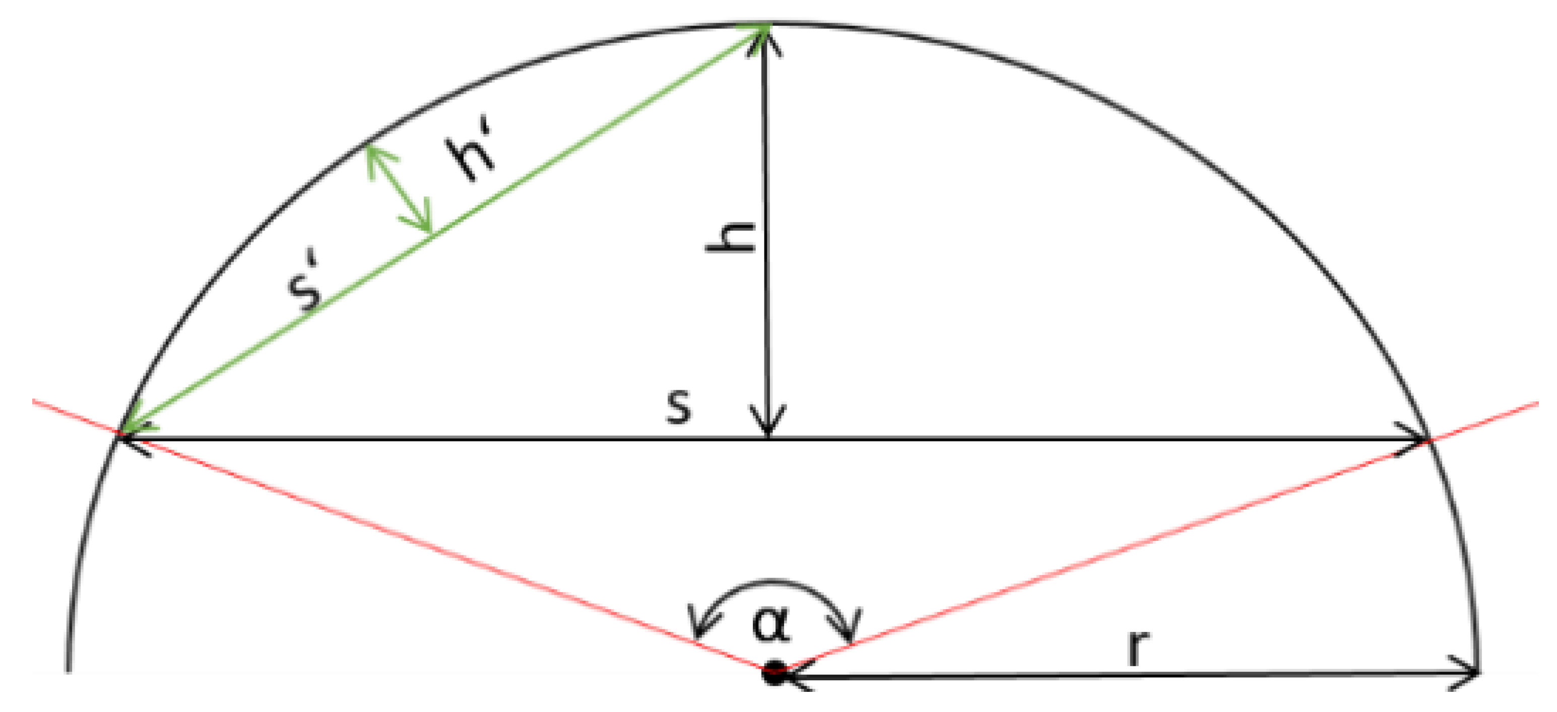
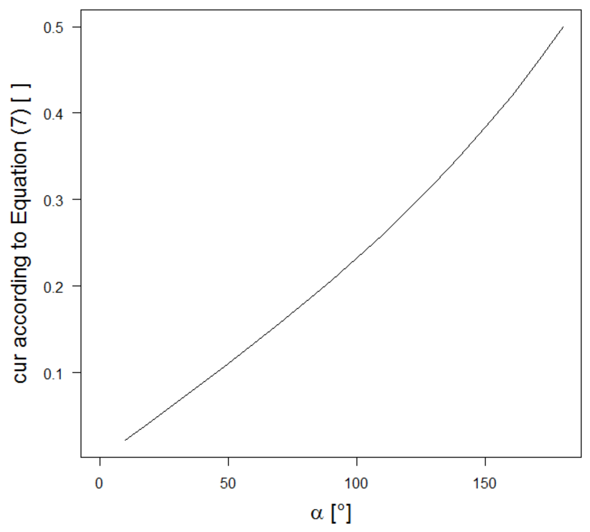
The other issue is that there are significantly higher curvature values for longer logs than for shorter stems and thus a comparison of different product range lengths with regard to the curvature is not possible with this method. In a theoretical model of an arc (Figure 9), the segment height h (equivalent to the bow height B) and the chord s (equivalent to the log length L) are in this case calculated using Equations (5) and (6). According to the current German curvature determination, the quotient formation from h and s (i.e., at log B/L) after shortening the radius (which means independent of the strength of the curvature) would result in Equation (7):

$$h=r(1-\cos (\frac{\alpha }{2}))$$

(5)

$$s=2r\sin (\frac{\alpha }{2})$$

(6)

$$cur=\frac{1-\cos (\frac{\alpha }{2})}{2\sin (\frac{\alpha }{2})}$$

(7)

If the curvature of this circle is now calculated as a function of the angle α (and thus also the segment length s representing a fictive log length), the value changes significantly (Figure 10). The higher α (and thus the longer the trunk), the higher the curvature value according to Equation (7) for an evenly sweeped log.

5. Conclusions

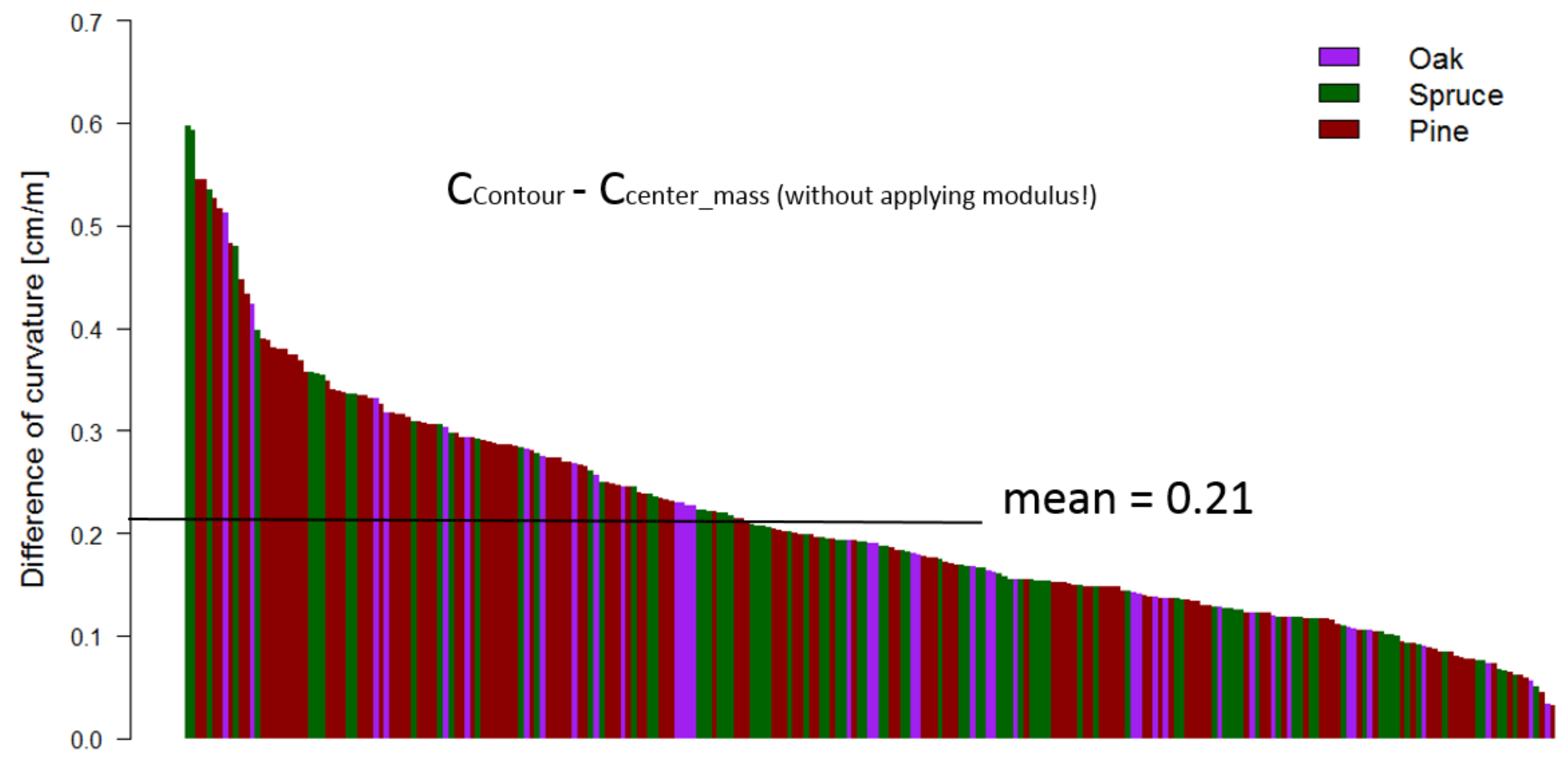
We showed that the two currently accepted calculation approaches described in the RV WV partly result in different ratings of the curvature of logs (expressed by relatively low correlations between them). This discrepancy could result in a diverging quality assessment (and thus finally pricing) of the same log dependent on which approach is used. Even if we could not detect a sawmill where the segment approach is currently applied, this fact should be taken into account in the ongoing development of the RV WV. When comparing the centerline approach (which is currently used in Austrian sawmills for the detection of bow heights) to the contour method (which is currently used in German sawmills), on average, we found 0.21 cm/m higher curvature values for the latter method. This difference can partly be explained by the effect of defects like bumps, branches or hollows in the log’s surface, which (even if the measured data is moderately smoothed) has stronger effects in the contour approach (Figure 8). Based on these findings, we would recommend the usage of the centerline approach for the calculation of the bow height in Germany as well, even if this would highly likely require the adaption of threshold for the quality assessment.

Further research is required regarding the effect of the calculation of the curvature value (e.g., bow height divided by log length or log diameter), which from our point of view could effectively be examined by using yield simulation [11,12,24]. Moreover, further studies could focus on integrating sweep types (e.g., described by Gjerdrum, Warensjö and Nylinder [23]) in the quality assessment. Meanwhile, it stays unregarded whether a log is symmetrical sweeped (“banana”) or a multiple sweeped with curves occurring in several layers. It can be assumed that, depending on the log geometry, the yield in the sawmill will vary considerably and a sweep that only occurs at the end of a log (e.g., root run-up) will have fewer negative effects on the end product than a log that is curved in several planes.