When Density Matters: The Spatial Balance between Early and Latewood

Abstract

Understanding the influence of the current climate on the distribution, composition, and carbon storage capacity of Mediterranean tree species is key to determining future pathways under a warmer and drier climate scenario. Here, we evaluated the influence of biotic and environmental factors on earlywood (EW) and latewood (LW) growth in Aleppo pine (Pinus halepensis Mill.). Our investigation was based on a dense dendrochronological network (71 sites), which covered the entire distribution area of the species in the Iberian Peninsula (around 119.652 km²), and a high-resolution climate dataset of the Western Mediterranean area. We used generalized linear-mixed models to determine the spatial and temporal variations of EW and LW across the species distribution. Our results showed an intense but differentiated climatic influence on both EW and LW growth components. The climatic influence explained significant variations across the environmental gradients in the study area, which suggested an important adaptation through phenotypic plasticity and local adaptation to varying climatic conditions. In addition, we detected a clear spatial trade-off between efficiency and safety strategy in the growth patterns across the species distribution. Additionally, in more productive areas, the trees presented a higher proportion of EW (more efficient to water transport), while, in more xeric conditions, the LW proportion increased (more safety to avoid embolisms), implying an adaptation to more frequent drought episodes and a higher capacity of carbon depletion. We therefore concluded that Mediterranean forests adapted to dryer conditions might be more efficient as carbon reservoirs than forests growing in wetter areas. Finally, we advocated for the need to consider wood density (EW/LW proportion) when modeling current and future forest carbon sequestrations.

1. Introduction

The geographical distribution of plant species in terrestrial ecosystems is a result of complex interactions between adaptations to climate and anthropogenic activity history [1,2]. Biodiversity, growth rates, and species distributions are expected to vary spatially with changes in the local temperature and water availability, as well as temporally, with wider changes in climate conditions [3]. Additionally, trees are sessile and long-lived organisms with a limited capacity to adapt to new environmental conditions, and consequently, the only possible mechanisms of acclimation they have to new environmental conditions are through its specific plasticity capacity. As a consequence of population isolation and/or differential selection pressures, local adaptations may lead to genetic differences between populations [4]. Phenotypic plasticity, defined as the range of phenotypes that the same genotype can express as a function of its environment [5], is expected to play a key role in the response of plants to rapid climate changes [6]. Species show a heterogeneous range of responses to climate variabilities, becoming the basis for potential adaptability to future climate conditions [3]. Besides, during the process of hydraulic structure construction, tree species plasticity is critically important, especially in drought-prone environments, such as in most areas of the Mediterranean [7,8].

Aleppo pine (Pinus halepensis Mill.) is one of the most representative tree species of the Mediterranean areas [9,10,11]. This species is specially adapted to the scarcity of water and occupies drought-prone areas where other species could not survive [12]. Different studies have highlighted the substantial phenotypic plasticity of Pinus halepensis in relation to different anatomical, reproductive, and vegetative traits [3,13,14] [Furthermore, a substantial plasticity in the annual rhythms of cambial activity has been established in response to different climatic conditions. Thus, some studies, such as Liphschitz et al. [15] or Prislan et al. [16], suggested that, under favorable climate conditions, the cambium is capable of maintaining its activity throughout the year. However, the activity of the cambium can stop between one and three months during the winter, depending on the prevalence of low temperatures [3]. In addition, during summer droughts, the cambial activity of Pinus halepensis may slow down or even stop and then resume when the moisture availability increases in the autumn. In other situations, there may be two stops in cambial activity: one in the winter caused by low temperatures and another during the summer caused by high temperatures and a lack of precipitation [17,18].

As a consequence of this plastic response to environmental conditions, growth rings with different anatomical characteristics are often formed [19]. In addition, an important variation in the frequency of these wood anatomical features has been described across the species’ range [20,21]. Thus, the likelihood of occurrence of absent rings (missing rings) increases especially in semi-arid and arid conditions [20], while the presence of intra-annual density fluctuations (IADFs) is maximized in the coastal areas of the Eastern Iberian Peninsula, where the thermal conditions in the autumn are still suitable for tree growth and the autumn is the main precipitation season [13].

Even though the presence of these wood anatomical features has been clearly established in previous research [19,21], little is known on the implication of these alterations in the functionality of the tree’s hydraulic system. The hydraulic system of Pinus halepensis, as in other conifers, consists of annual rings whose cells can be morphologically divided into two types of seasonal wood: earlywood (hereafter abbreviated as EW), which is normally formed in the spring and early summer and is characterized by tracheids with wide lumen and thin walls, and latewood (hereafter abbreviated as LW), which is formed in the summer and autumn and is characterized by tracheids with narrow lumen and thick walls [8,22,23]. The functionality of xylem for water transport is conditioned by the type of cells (i.e., EW and LW tracheids) present in the tree ring [24], but despite its importance, few studies have focused on how environmental conditions affect the EW/LW proportion in forest populations.

The plasticity and sensitivity of Pinus halepensis to climatic variations have been well-studied by the scientific community, as have the growth patterns throughout its range [3]. Extensive literature on the biogeography and ecology of Pinus halepensis [25,26], as well as dendroclimatic analyses at specific localities in the Mediterranean Basin [27,28,29], support this theory. Yet, there are no regional studies on the effect of climatic conditions on EW and LW growth, leading to a lack of studies on wood growth patterns across the species distribution. There are studies, however, for other species, such as that of reference [30], where they analyzed the characteristics of the earlywood vessels of Pyrenean oak (Quercus pyrenaica Willd.) and Pedunculate oak (Quecus robur) under the hypothesis that, even when growing under the same climatic conditions, the effect of the climate on earlywood formation is different between them. An additional study by reference [31], also for Quercus pyrenaica, addressed the relationship between climate and wood formation, obtaining relevant results related to micro-, meso-, and macroclimatic conditions and pointing to the existence of cause–effect relationships. Yet, none of these studies addressed this issue from the perspective of wood growth patterns. Dendrochronology is a powerful tool to retrospectively study the growth patterns of trees and to analyze geographical variations or changes in their EW/LW structures. The use of dense dendrochronological networks is necessary to explore the differential responses of each of the populations in different climatic and environmental conditions [12].

In this study, we used a dense dendroclimatic dataset of Pinus halepensis covering the ecological gradient in peninsular Spain composed by samples from 71 sites with EW and LW measures for each tree ring. A high-resolution climatic dataset (5 × 5 km) covering the species’ real distribution facilitated the investigation about the variability of the relationship between EW/LW formation and the climate.

Our objectives were (1) to evaluate the climatic influence on EW and LW growth in a network of Pinus halepensis occupying the distribution of the species in the Western Mediterranean and (2) to describe the geographical patterns of distribution of EW and LW growth and the fraction of both along with the distribution of the species. These climatic signals are discussed and interpreted from the point of view of the plasticity and adaptability of the species in the context of climate change, interpreting how these patterns could affect, in addition, the carbon balance.

2. Materials and Methods

2.1. Materials

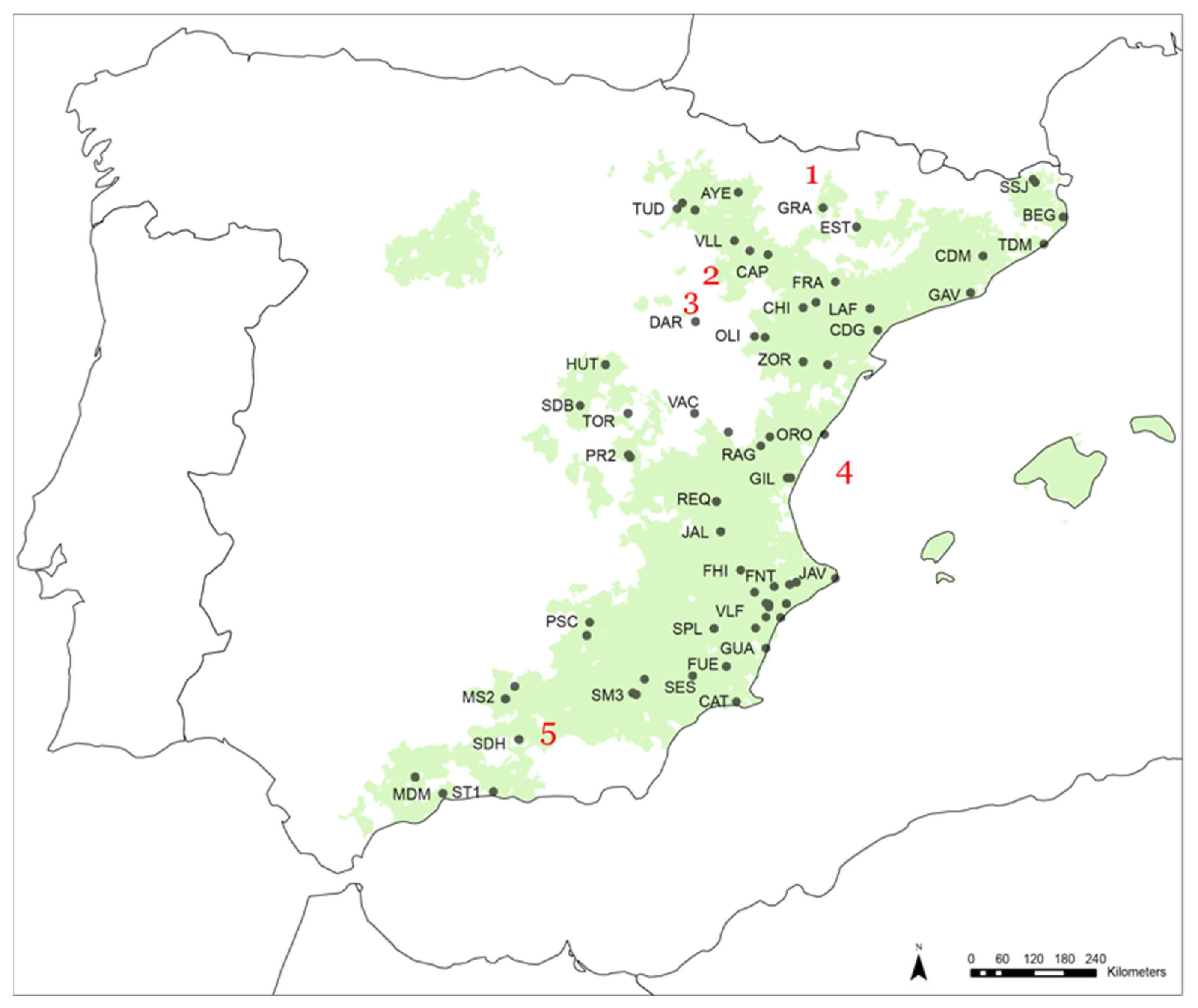
2.1.1. Dendroclimatic Dataset

The study area was located in the Mediterranean region of the Iberian Peninsula, where we sampled and compiled ring width information from 71 Pinus halepensis forests areas (Figure 1) (about 119.652 km² covered). At each site, mature, healthy, and dominant trees were selected and sampled at breast height between 2001 and 2014 [21]. The range of altitudes that included the dendrochronological dataset varied from 1 to 1676 m.a.s.l. (Table S1).

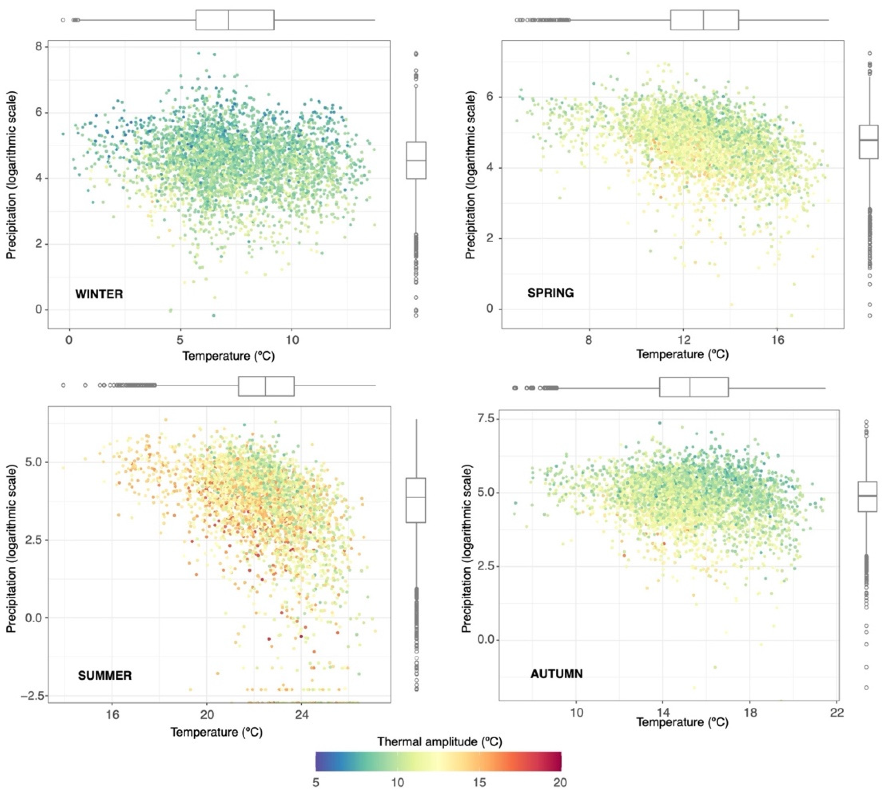
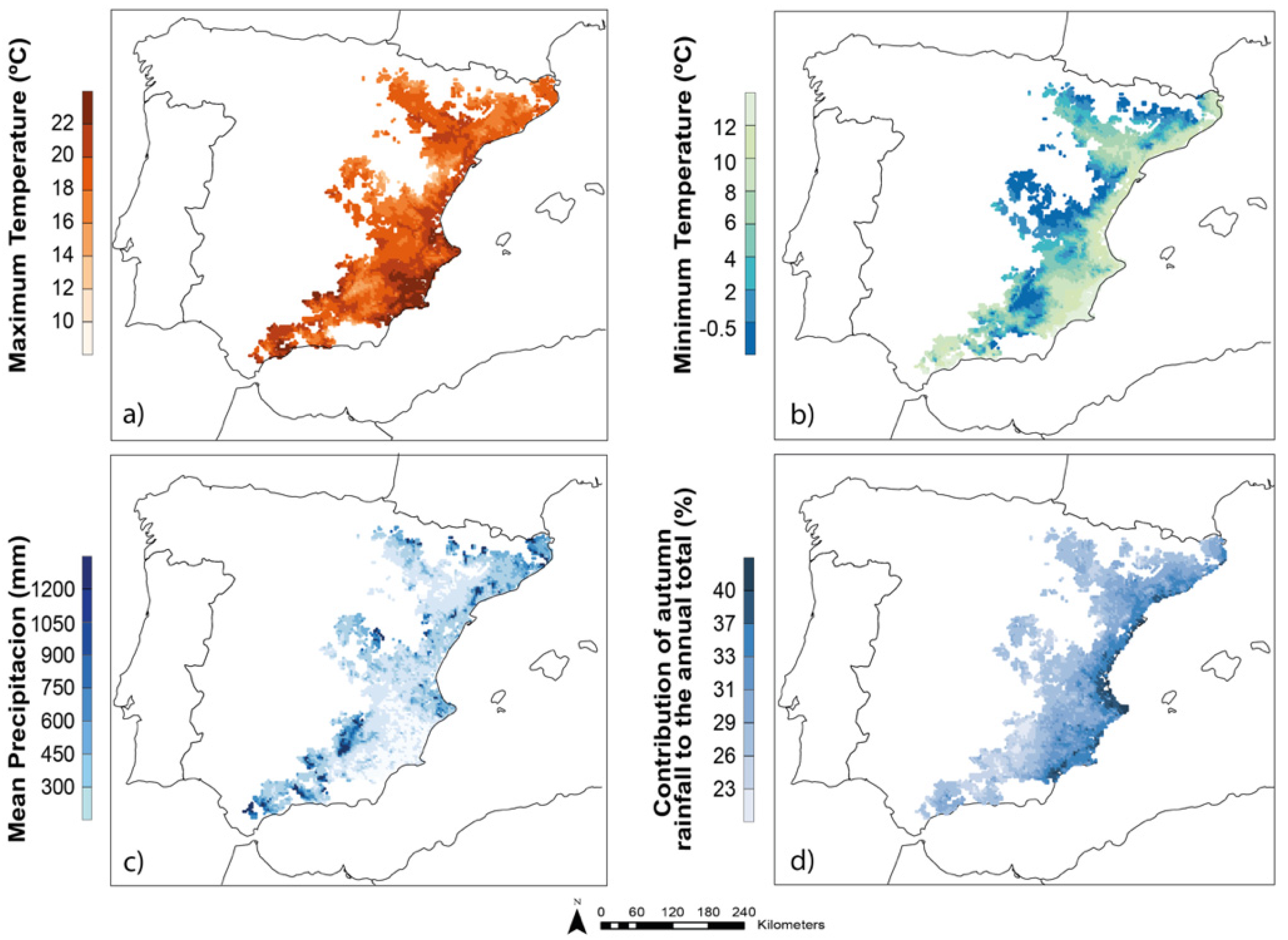
2.1.2. Climatic Domain and Sources

The average monthly temperature and the total monthly rainfall of each sampling site were obtained from the high-resolution datasets STEAD [32] and SPREAD [33], respectively. These two new daily gridded datasets were created using all the available climatic information (>12,000 precipitation and >5000 temperature stations) covering the whole Spanish territory over the 1950–2012 period. The average annual precipitation and temperature were calculated from September of the previous year to August of the current year and described the climatic conditions during the year of each tree-ring formation.

A Mediterranean influence prevailed in the climatic characteristics, with soft winters and hot summers. Precipitation was highly variable both within the year and between annual values, with two peaks in the autumn and spring. Summertime was typically dry, and the net budget of potential water balance (precipitation–evapotranspiration) was negative all year, except in higher elevations (>1000 m.a.s.l.). Temperatures were higher in coastal areas, decreasing towards the inland and high elevation zones. The typical average values ranged from 13 to 16 °C, but there existed a large variability depending on the area and the season (Figure 2). In this context, seasonal thermal amplitude (difference between the maximum and minimum temperatures) can range from 5 to almost 20 °C, lower values occurring in the winter, when temperatures were more homogeneous across the territory, and the higher ones in the summer, when the differences were larger due to the different atmospheric dynamics of the mountain and coastal areas and because of the aforementioned sea softening. Overall, precipitation was scarce in most of the study area (average of 492 mm), with frequent values below 300 mm at southeast and northern inland zones (Figure 3). Differences in the climatic features were emphasized during the summer, when lowlands suffered high hydric stress with average temperatures over 22 °C and almost nonexistent precipitation, and mountain areas, when convective storms were prevented by raising temperatures, acting as refuges for biological activity.

2.1.3. Dendrochronological Methods

The trees were sampled from one to three times each, depending on the tree’s condition, using an increment Pressler borer. The samples collected on the field were identified with working marks, which encompassed the location, tree species, and number of trees, to be later easily recognizable between each other and transported to the laboratory. Later, the cores were mounted on wooden supports, air-dried, and the transversal surface of the samples were sanded and polished with a belt sander using progressively finer sandpaper, from 80, 120, 180, 220, or 280 grit until the tree rings were perfectly visible under a microscope. The prepared samples were scanned with a Mustek S-series 2400 Plus flatbed scanner with a resolution at 1200 dpi. Later, the cores were visually cross-dated using the CDendro&CooRecorder 9.4 program [34]. This program recognizes the tree rings on a calibrated high-resolution digital photo of a sample and allows to manually cross-date tree rings. Finally, COFECHA software was used for its verification [35].

Tree ring width measurements were done to the nearest 0.01 mm with TSAPW-Win^TM Scientific software and a LINTAB^TM5 measuring device (Rinntech, Heidelberg, Germany, www.rinntech.com, accessed on: 25 April 2021). EW and LW measurements were performed following Mork’s formula (Mork 1928). Mork considered a LW tracheid to be one in which the width of the common wall between the two neighboring tracheids multiplied by two was equal to, or greater than, the width of the lumen. When the value was less than the width of the lumen, the xylem was considered to be EW [36].

Finally, a total of 1026 trees were sampled at different locations in the Iberian Peninsula. The range of diameters at breast height (Figure 4d) of the sampled trees oscillates were between 10 and 80 cm, with a higher frequency of trees between 20 and 30 cm. Globally, the EW and LW of a total of 139,634 growth rings were measured (Figure 4a,b). The EW ratio varied in a large proportion of tree rings, between 0.6 and 0.9 (Figure 4c). The maximum frequency was obtained at 0.8, and only 2% of the rings had a LW ratio higher than the EW ratio (ratio < 0.5).

2.1.4. Dendrochronological Dataset

The cambial age at breast height of the cores where the pith reached was calculated directly from the count of the annual growth rings of the sample. In contrast, when the cores lacked pith or measurements were obtained from external sources, pith displacement estimates were obtained by fitting a geometric pith locator to the innermost ring. After calculating the missing rings to the pith, the cambial age was estimated by adding the rings counted in the oldest sample of the individual and the estimated missing rings.

Then, after obtaining the necessary EW and LW information for each of the rings, the basal area (BA) was calculated. The early and latewood tree ring width value measurements were transformed into basal area increments (BAI_EW and BAI_LW), where the geometric constraint of adding a volume of wood to a stem of the increasing radius was taken into account [37].

The BAI series for each tree was obtained by applying the following formula:

$${\mathrm{BAI}}_{\mathrm{t},\mathrm{y}}= \mathsf{\pi }\left({\mathrm{r}}_{\mathrm{t},\mathrm{y}}^2-{\mathrm{r}}_{\mathrm{t},\mathrm{y}-1}^2\right)$$

(1)

where r_t and ${\mathrm{r}}_{\mathrm{t},\mathrm{y}-1}^2$ correspond to the stem radii corresponding to tree t for years and y − 1 respectively. Finally, an average BAI series was calculated for each specimen by averaging the BAI series of the cores corresponding to each tree.

For each study site, the mean monthly temperature and total monthly precipitation were obtained from the closest grid point to each sampled site, obtaining a set of high-resolution SPREAD and STEAD [32,33]. In order to describe the climatic conditions during the year of formation of each ring, the annual precipitation and the mean annual temperature (from the previous September to current August) were calculated. Since high-quality climate data in the study areas was limited starting from the second half of the 20th century, the dendroclimatic dataset and further analyses were limited to the common period (1950–2014).

In order to highlight the climatic gradient marked in the study area, the total annual precipitation and mean annual temperature were combined into a single simple parameter that could represent the measure of the precipitation efficiency. For this purpose, the aridity index (AI) proposed by De Martonne (1936) (42) was used, calculated using the following formula:

$$A{I}_{s,y}=\frac{P_{s,y}}{10+T_{s,y}}$$

(2)

where Ps,y is the total precipitation (in mm) given at site s in y, and Ts,y is the mean annual temperature (in °C) recorded at site s in year y. The different climate types defined by the IA are arid (0–10), semi-arid (10–20), Mediterranean (20–24), semi-humid (24–28), humid (28–35), very humid (35–55), and extremely humid (>55).

2.2. Statistical Analysis

Models

Generalized linear mixed-effects models (GLMM) using a Gamma distribution of the errors were used to describe the spatial and temporal variations in earlywood (BAI_EW) and latewood (BAI_LW) throughout the species’ distribution. We use the statistical computing environment R and the package lme4 [38]. This model was based on the period 1950–2012 due to the common availability of the climate and dendrochronological data:

$$\begin{gathered} BAI\_E{W}_{i,t}=\beta +A{I}_{mean}+EW{p}_{i,t-1}+Cli{m}_t+(A{I}_{mean}\ast Cli{m}_t)+\left(EW{p}_{i,t-1}\ast Cli{m}_t\right)+(\left(BA{I}_{EW}{}_{i,t-1} \\ +BA{I}_{LW}{}_{i,t-1}+B{A}_{i,t-1}\right) | TreeCod{e}_i) \end{gathered}$$

(3)

$$\begin{gathered} BAI\_L{W}_{i,t}=\beta +A{I}_{mean}+EW{p}_{i,t-1}+Cli{m}_t+(A{I}_{mean}\ast Cli{m}_t)+\left(EW{p}_{i,t-1}\ast Cli{m}_t\right)+(\left(BA{I}_{EW}{}_{i,t} \\ +BA{I}_{LW}{}_{i,t-1}+B{A}_{i,t-1}\right) | TreeCod{e}_i) \end{gathered}$$

(4)

where BAI_EW_i,t and BAI_LW_i,t represent the basal area increment of earlywood and latewood, respectively, of the tree i during year t. The intercept of the models is β. The independent variables included are (a) the mean aridity index (AImean), representing a general descriptor of the mean climate conditions for each location, (b) the proportion of earlywood existing in the whole tree in the previous year of the tree ring formation $(EW{p}_{i,t-1}),$and (c) the set of climate conditions occurred during the year t where the tree ring of tree i was formed. Such a set included 12 variables representing the precipitations that occurred for each season, and the seasonal mean of the maximum and minimum temperatures. The interaction between the AImean and the $EW{p}_{i,t-1}$ factor against the climate variable was also included in the models, since it has been proved that there are potential variations in the climate influences across different climate regions, and it modulates the climate sensitivity of trees [39]. In addition, since it is well-known that the radial growth of a tree varies as it gets older/larger, and it is also influenced by the growth account in the previous year, we included the basal area of the tree in the previous year ($B{A}_{i,t-1})$, as well as the basal area increments of EW and LW in the previous year, as random terms in the model. The code of each tree was used as the random factor in order to account for variations in the specific growth of each individual tree. Both dependent and independent variables were log-transformed when needed to ensure a normal distribution. In addition, to ensure a balanced weighing of each of the independent variables, all of them were standardized (to have a zero mean and a standard deviation of 1) prior to the construction of the models. The model was built on the basis of the information corresponding to the period 1950–2012 due to the common availability of the sampled tree ring measurements and the climatic data used. These models were evaluated by comparing the full model with a model including only the intercept and with the models without the three groups of independent variables (AI, EWp, and climatic factors).

The applicability of the model to the total range of the species was done by establishing a theoretical tree with an initial BA-EW and BA-LW size of 1 cm and an initial EWp value of 0.5. This theoretical model was applied to the climatic conditions obtained for the year 1951, the results of which modified the size of the trees and the EW ratio. These new obtained conditions were applied in the models of all the years that made up the study.

The sum of all the growth data obtained from the 62 years of simulation provided a spatially comparable estimate of the mean annual growth, at least in terms of the structural conditions of the populations (same initial conditions).

3. Results

3.1. Main Factors Controlling EW and LW Growth in Pinus Halepensis

The spatial and temporal variations in the secondary growth of EW and EW of Pinus halepensis across its distribution area of Spain can be suitable explained using climatic and weather variations across the area (

Table 1. Prediction model results for earlywood (Left) and latewood (Right). * (p < 0.05); ** (p < 0.01); *** (p < 0.001).

	Earlywood BAI			Latewood BAI
	Estimate	Std. Error	sig	Estimate	Std. Error	sig
(Intercept)	2.75 × 100	6.46 × 10−4	***	2.65 × 100	6.65 × 10−4	***
Aridity gradient (AI)	−1.19 × 10−2	7.06 × 10−4	***	−3.96 × 10−3	7.04 × 10−4	***
Earlywood proportion (Ep)	2.96 × 10−3	4.70 × 10−4	***	−6.66 × 10−3	4.37 × 10−4	***
AI: Ep	3.70 × 10−3	5.89 × 10−4	***	1.21 × 10−3	5.26 × 10−4	*
PP Autumn-1	1.12 × 10−2	2.52 × 10−4	***
PP Win	1.25 × 10−2	2.68 × 10−4	***	7.89 × 10−4	2.43 × 10−4	**
PP Spr	1.19 × 10−2	2.72 × 10−4	***	1.50 × 10−3	2.52 × 10−4	***
PP Summer	3.86 × 10−3	2.59 × 10−4	***	5.70 × 10−3	2.36 × 10−4	***
PP Autumn				6.56 × 10−3	2.29 × 10−4	***
Tmax Autumn-1	−9.37 × 10−4	6.39 × 10−4
Tmax Win	1.84 × 10−4	7.08 × 10−4		−3.77 × 10−3	6.47 × 10−4	***
Tmax Spr	−8.18 × 10−3	6.50 × 10−4	***	4.74 × 10−3	5.55 × 10−4	***
Tmax Summer	3.39 × 10−4	5.37 × 10−4		−3.89 × 10−3	5.04 × 10−4	***
Tmax Autumn				−1.27 × 10−3	5.98 × 10−4	*
Tmin Autumn-1	−7.21 × 10−3	9.58 × 10−4	***
Tmin Win	7.27 × 10−3	6.69 × 10−4	***	2.44 × 10−3	5.99 × 10−4	***
Tmin Spr	2.58 × 10−3	9.45 × 10−4	***	−5.68 × 10−3	8.51 × 10−4	***
Tmin Summer	−5.92 × 10−3	8.85 × 10−4	***	2.74 × 10−3	8.43 × 10−4	**
Tmin Autumn				7.21 × 10−3	9.46 × 10−4	***
AI: PP Autumn-1	−3.46 × 10−3	2.65 × 10−4	***
AI: PP Win	−4.44 × 10−3	2.84 × 10−4	***	4.31 × 10−4	2.62 × 10−4
AI: PP Spr	−2.20 × 10−3	2.65 × 10−4	***	−1.70 × 10−4	2.46 × 104
AI: PP Summer	−1.50 × 10−3	2.56 × 10−4	***	1.42 × 10−4	2.33 × 10−4
AI: PP Autumn				−2.68 × 10−3	2.42 × 10−4	***
AI: Tmax Autumn-1	−1.15 × 10−3	6.84 × 10−4
AI: Tmax Win	5.53 × 10−3	7.53 × 10−4	***	1.38 × 10−3	6.86 × 10−4	*
AI: Tmax Spr	3.77 × 10−3	7.00 × 10−4	***	−1.62 × 10−3	6.00 × 10−4	**
AI: Tmax Summer	−4.86 × 10−3	5.93 × 10−4	***	2.01 × 10−3	5.60 × 10−4	***
AI: Tmax Autumn				−1.61 × 10−3	6.47 × 10−4
AI: Tmin Autumn-1	1.48 × 10−4	1.05 × 10−3				*
AI: Tmin Win	−1.07 × 10−3	7.25 × 10−4		−1.78 × 10−3	6.47 × 10−4	**
AI: Tmin Spr	−5.99 × 10−3	1.01 × 10−3	***	2.10 × 10−3	9.02 × 10−4	*
AI: Tmin Summer	6.19 × 10−3	9.50 × 10−4	***	−1.23 × 10−3	9.07 × 10−4
AI: Tmin Autumn				7.42 × 10−4	1.03 × 10−3
Ep: PP Autumn-1	−3.01 × 10−4	2.63 × 10−4
Ep: PP Win	2.16 × 10−4	2.83 × 10−4		5.30 × 10−4	2.55 × 10−4	*
Ep: PP Spr	−3.20 × 10−4	2.71 × 10−4		5.64 × 10−4	2.51 × 10−4	*
Ep: PP Summer	−3.90 × 10−4	2.56 × 10−4		−1.13 × 10−3	2.32 × 10−4	***
Ep: PP Autumn				2.63 × 10−4	2.37 × 10−4
Ep: Tmax Autumn-1	1.50 × 10−4	6.50 × 10−4
Ep: Tmax Win	−8.95 × 10−4	7.16 × 10−4		1.93 × 10−3	6.53 × 10−4	**
Ep: Tmax Spr	1.35 × 10−3	6.70 × 10−4	*	−1.20 × 10−3	5.73 × 10−4	*
Ep: Tmax Summer	1.83 × 10−4	5.42 × 10−4		−9.88 × 10−5	5.03 × 10−4
Ep: Tmax Autumn				8.41 × 10−4	6.17 × 10−4
Ep: Tmin Autumn-1	1.46 × 10−3	1.00 × 10−3
Ep: Tmin Win	4.33 × 10−3	6.98 × 10−4	***	7.77 × 10−4	6.22 × 10−4
Ep: Tmin Spr	−4.32 × 10−3	9.93 × 10−4	***	−3.43 × 10−4	8.90 × 10−4
Ep: Tmin Summer	−1.57 × 10−3	8.89 × 10−4		1.56 × 10−3	8.34 × 10−4
Ep: Tmin Autumn				−1.31 × 10−3	9.79 × 10−4

).

Precipitation from the previous autumn, winter, and spring were especially important in the growth of EW. Summer precipitation was also significant, although with less relative importance. In LW, the most important climatic factors explaining the temporal and spatial variations in growth were the summer and autumn precipitation, although the winter and spring rains were also significant.

The influence of the maximum and minimum temperatures was of lesser relative importance, although their effects on growth were also significant. In this respect, the growth of EW was favored when/where the minimum temperatures of autumn and summer were low but the minimums in winter and spring were elevated, and the maximums in spring were also low. The patterns of influence of temperature on LW growth were nearly reversed. The growth of LW was favored when/where the minimum temperatures were high and maximum temperatures low in the winter, summer, and autumn. The influence of spring temperatures was also significant but with a contrary signal. Thus, LW growth was enhanced when/where the minimum temperatures in the spring were low but the maximum were high.

Despite the existence of the previously defined general climate influence, our analyses revealed that the influences of both the seasonal precipitation and the seasonal temperatures were not homogeneous across the aridity gradient of the species distribution. In the EW portion, precipitation had a significant influence, but its importance was more pronounced in the more arid sectors (as we could interpret by the negative interactions between the precipitation of all seasons and aridity gradient). The relative importance of the temperatures also varied across the aridity gradient. A greater influence could be observed from the winter and spring maxima in the humid sectors and a greater influence from the summer maxima in the more arid sectors. As for the summer minimums, a greater influence was observed in humid areas, while, in the more arid sectors, the spring minimums had the greatest influence. Furthermore, the differential effect of the temperatures along the aridity gradient of LW growth caused a greater influence of the winter and summer maxima in the humid sectors, while the spring and autumn maxima had a greater influence on the more arid sectors. A greater influence of the spring minima could also be obtained in humid sectors and a greater influence of the winter minima in the more arid sectors.

The climatic variations revealed a pronounced effect on the tree growth variations, but our analyses also revealed that the wood structural characteristics of the trees had a significant effect on tree productivity. Thus, the trees with a larger proportion of EW tended to produce a wider EW section, and the trees with a wider LW section tended to produce a wider LW section. Interestingly, the importance of the influence of such anatomic characteristics of the tree was higher in humid environments (as we could interpret by the positive signals of the interaction between the aridity gradient and the EWp).

The EW/LW structure of a tree also alters, although partially, the climate and growth relationships. Thus, the influence of the winter minimums was greater in trees with a higher percentage of EW, while the influence of the spring minimums was greater in trees with lower percentages of EW. In addition, the summer rainfall was particularly influential on trees with low EWp.

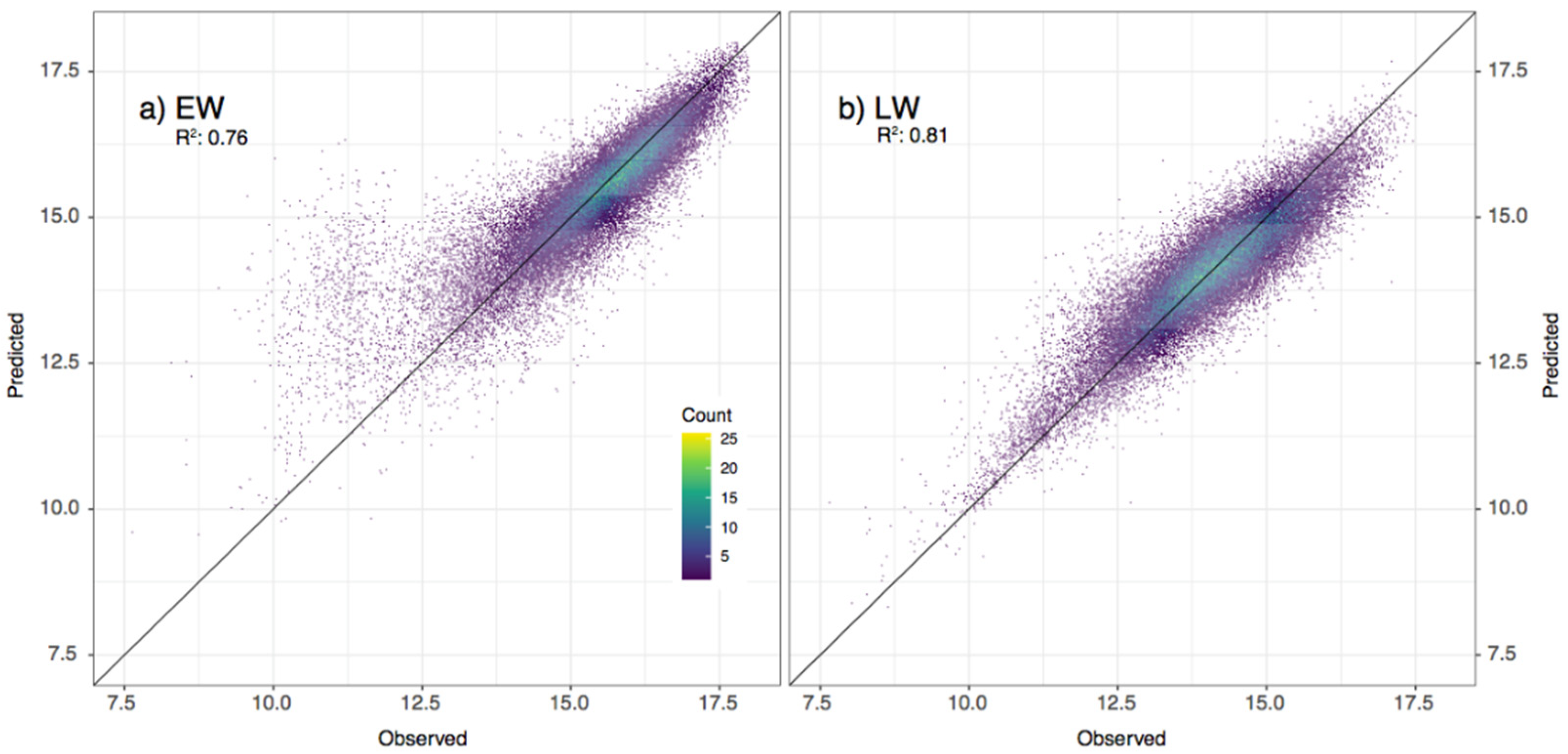
3.2. Models’ Accuracy Assessment and Validation

To evaluate the accuracy of the growth models, we followed the previous approaches [12,40] by comparing the model with all the explanatory variables (full model) with its reduced versions, i.e., without the EWp, AI, and climatic factors, respectively, and with the model only built with the intercept (null model). We performed this comparison both in EW and LW through a set of probabilistic statistical measures (

Table 2. Accuracy assessment of the models. Goodness-of-fit measures: AIC (Akaike information criterion), BIC or SBC (Schwarz’s Bayesian criterion), logLik (log-likelihood function), deviance (Residual deviance), and df.resid (Degrees of freedom—Residual).(Table S2).

		AIC	BIC	logLik	Deviance	df.resid
Earlywood	Full	102,951.6	103,402.9	−51,424.8	102,849.6	51,435
	Null	115,841.8	115,948.0	−57,908.9	115,817.8	51,474
	no AI	104,370.0	104,697.4	−52,148.0	104,296.0	51,449
	no Ewp	103,000.0	103,327.4	−51,463.0	102,926.0	51,449
	no Clima	115,767.0	115,899.8	−57,868.5	115,737.0	51,471
Latewood	Full	79,472.3	79,799.7	−39,699.1	79,398.3	51,449
	Null	82,315.1	82,421.3	−41,145.6	82,291.1	51,474
	no AI	79,919.5	80,247.0	−39,922.8	79,845.5	51,449
	no Ewp	79,710.7	80,162.1	−39,804.4	79,608.7	51,435
	no Clima	82,665.0	82,797.7	−41,317.5	82,635.0	51,471

) in order to quantify the model performance (AIC, BIC, log-likelihood, and deviance) and complexity (degrees of freedom).

The results showed the lowest values in the full models both in EW and LW, meaning that, despite the highest complexity, the joint consideration of the AI, EWp, and climatic factors better represented the growths of the trees than omitting any of the explanatory variables.

The full models of EW and LW were then applied to the observations, and we performed a comparison between the observations and their corresponding predictions to evaluate their goodness-of-fit (Figure 5). The results showed a good agreement, with coefficients of determination of 0.76 and 0.81 for EW and LW, respectively. No general bias was observed in both sets of predictions, except for a slight overestimation of a few observations in EW lower than 12.5. Despite the inherent limitations related to models’ uncertainties, the applicability of the obtained models all across the distribution area was possible given the agreement between the predicted and observed wood measurements. However, the results were applicable to the studied species in the study area and should not be extrapolated to other species or sites.

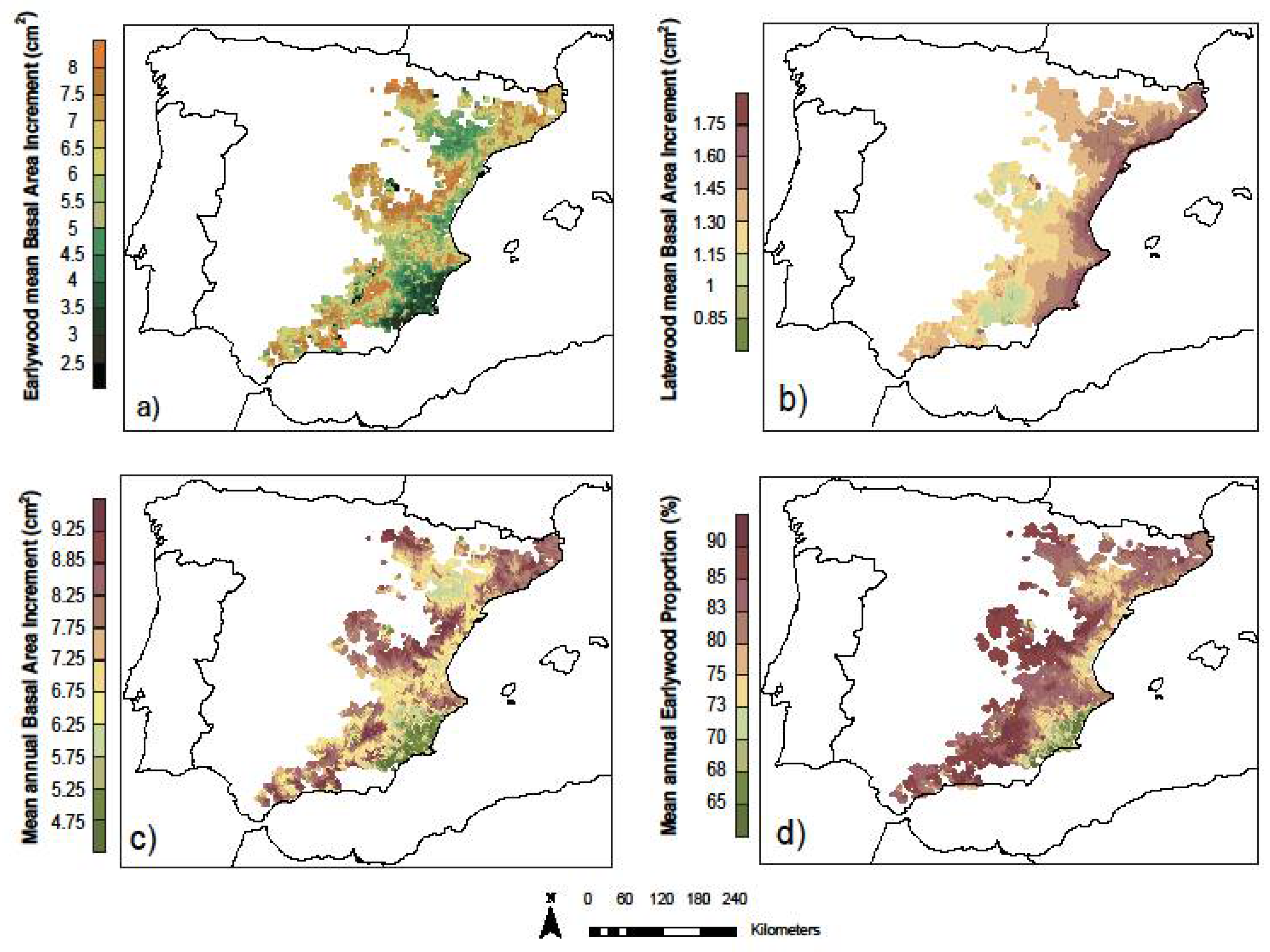
3.3. Models’ Predictions across Species Distribution

The final models obtained were used to describe the performance of EW and LW growths across the species distribution in the Iberian Peninsula. To obtain comparable results across the study area, the models were applied to the observed climate conditions of 1951 of each pixel for a theoretical tree with an initial basal area of 2 cm² (1 cm² corresponding to the EW section and another 1 cm² of LW) and, then, an initial EWp of 0.5. Predicted growths at each pixel for 1951 were added to such initial tree conditions, and then, the model was applied again subsequently to years 1952–2012. The sum of all the growth data obtained from the 62 years of the simulation provided a spatially comparable estimate of the mean annual growth across the distribution area. The resulting patterns of the growth estimates of the EW basal area, LW basal area, annual basal area, and EWp are shown in Figure 6.

The EW growth (Figure 6a) values were lowest in the semi-arid areas of SE Spain, with the second area of low EW production in the central sector of Ebro Valley, associated, in both cases, with low precipitation values and high summer temperatures, factors that act as growth-limiting factors. From these two sectors, a progressive increase in the EW growth values was observed towards the highest areas of the study area, such as the areas of Western pre-Pyrenees and the Catalan Coastal Mountain Range in the north, the sectors of the Iberian system closest to the Mediterranean, and those with the greatest exposure to westerly flows, as well as in the south in areas of the Betic and Penibetic Mountain Ranges, which also offered good exposure to westerly flows. This corresponded to the elevated areas where the temperature did not usually act as a limiting factor and where, on the other hand, the winter and spring precipitations were more abundant, influencing the development of the cambium during this period and, therefore, the formation of EW.

In relation to the growth of LW (Figure 6b), the spatial distribution patterns changed markedly from those indicated for EW. The entire Mediterranean coastline offers higher LW growth values, which progressively decrease towards inland, reaching the lowest values in the most continental and higher elevation areas. These high LW growth values correspond to areas with high autumn temperatures and higher autumn rainfall, often annual maxima. Under these conditions, secondary growth is prolonged throughout the season and, in some cases, even reactivated after a break caused by high temperatures and summer drought. As we pointed out, towards the interior, the LW growth decreases, especially in the more continental and higher altitudinal areas but, above all, in those more westerly and more exposed to ocean fronts, where the autumn maximum of precipitation loses importance compared to the spring maximum.

The distribution of the EW fraction (Figure 6c) combines and highlights the spatial patterns seen above for EW and LW. The areas with milder spring and summer temperatures and a higher presence of winter and spring precipitation, i.e., the westernmost areas of the Pinus halepensis distribution in the Iberian Peninsula, have the highest RW fractions, above 0.8 and even 0.9. In these areas, the radial growth has adapted to the most favorable climatic conditions during the beginning of the growing season, generating, as we can see, most of the secondary growth during that time of the year. In contrast, the warmer and drier areas at the southeast of the peninsula have the lowest EW fraction, below 0.7. Hot and dry summers combined with mild autumns and higher convective activity in the Mediterranean, and, therefore, more precipitation that favor the development of the cambium in the final stages of the growing season, generate a higher number of LW cells.

Finally, RW width is conditioned mainly by EW width (Figure 6d). Although the LW growth was high in the dry and warm areas at the SE of the peninsula, it did not exceed 65% of the total basal area increment in any case, with most of the territory having values above 80% (Figure 6a,b). This means that the total growth and the EW growth showed practically similar spatial patterns, with lower average annual growths at the SE and the central sector of Ebro Valley, where low rainfall at any time of the year together with high summer temperatures had a significant effect on growth, while the highest growth rates, 120% higher, were observed in areas with milder temperatures due to their higher altitudes and better orientation to oceanic flows that ensured greater volumes of precipitation during the spring.

4. Discussion

4.1. Tree Acclimation and Spatial Plasticity in Secondary Growth

Pinus halepensis represents a key species across the Mediterranean area, being one of the better-adapted species to survive in dry and semiarid areas [12,41,42]. The ecology and biogeography of Pinus halepensis have been widely studied, as well as the influence of climate variability on its secondary growth [3,10,19,27,28,43]. Usually, cambial phenology and secondary growth patterns of Pinus halepensis are primarily linked to precipitation variability, and yet, different studies have demonstrated that temperature variations can also have a significant influence [3,8,16,20].

From a functional hydraulic point of view, there are basically two distinct cell types within a tree ring in conifers: The early season growth in a tree produces EW cells that are wide in diameter with a thinner cell wall and generally accounts for 40–80% of the ring’s growth in width. Then, during late spring or early summer, as the moisture stress increases, auxin production decreases, triggering the formation of smaller but denser LW cells [18,44]. As a consequence, EW formation has been traditionally described to be less sensitive to climate variability than the LW zone [45,46].

Climate seasonality has a strong influence on the annual tree growth but, also, on the wood anatomical characteristics of the cells formed and, also, on the wood properties and hydraulic functionality of the formed tree ring [19]. Our results for Pinus halepensis across its distribution area in the Iberian Peninsula, comprising a wide set of climate conditions, partially agreed with these general descriptions. Henceforth, we found that both EW and LW cell formation were strongly sensitive to climate variability. In addition, such sensitivity and the seasonality of such influences plastically differed across the climate gradients in the distribution area. The climate conditions of the previous autumn had a significant influence on EW formation, suggesting that the formation of the EW section depends partially on the carbohydrates synthesized in the previous year [47,48], while the formation of LW depends on the climate conditions and then on the photo assimilates synthesized during the current year [49].

In addition, and similar to what was described for the total annual ring growth [3], the sensitivity and the seasonality of how climate influences plastically differ across the climate gradients in the area also suggest a strong ability of Pinus halepensis to modulate the growth during the different seasonal phases according to the different environmental conditions. In fact, the sensitivity to climate variations and, especially, to the varying soil humidity conditions varied geographically, being higher in dry and semiarid environments [40,50,51]. As a consequence of such plastic characteristics, the proportion of EW versus LW within the tree rings strongly varied across the species distribution: from 90% of EW cells in the wood formed at mesic environments to less than 65% in thermo-Mediterranean semiarid environments.

This spatial pattern agreed with studies on xylogenesis on the species that suggested that cambial activations and the start of the growing season are usually delayed in mountain environments. However, drought stress conditions are also delayed in mountain areas in comparison to coastal sites, and as a consequence, the duration of xylogenesis for EW cell formation was similar across the distribution area [18,52]. Despite a similar length of the EW growing season, the growth rate in mesic environments was higher basically due to the higher water availability. Conversely, the length of the period for LW formation may strongly differ spatially since, after the slowdown of the cambial activity during the summer, cambial reactivation was only possible when and where favorable (i.e., wet and warm) conditions occurred during the autumn [21]. Across the species distribution in the IP, such favorable conditions occurred more commonly at the coastal areas [21,53], explaining why higher latewood growth rates were observed at the coastal areas.

4.2. Differing Anatomical Strategies

It is well-known that tree species with long organs and reserves show a slower acclimation response to today’s climatic variations than species with shorter lives [54]. The hydraulic conductivity is closely related to sapwood condition and contributes to the efficiency of water transport, reducing the tree’s risk of water deficits and promoting growth. In this respect, and given that EW and LW cells are hydraulically functional for decades, differences in the EW/LW patterns, as described in our results, have important consequences that define the differential abilities of Pinus populations in both the efficiency of their hydraulic capacity and their safety characteristics when responding to drought conditions.

EW cells have approximately 11 times the specific water conductivity of latewood cells, and, as a consequence, up to 90% of the total flow occurs through EW [24]. Therefore, trees with a higher proportion of EW will, in turn, have a wide sapwood, which will allow for increased water flow, resulting in an efficient growth strategy and, at the same time, a slower response to climatic variations. This slower response will allow the tree to maintain a growth rate despite adverse climatic conditions. The trade-off, however, is that EW ducts with a high conductivity may be more vulnerable to embolism [55,56,57]. Conversely, a higher proportion of latewood cells and, thus, a narrower sapwood reduces the growth efficiency, leading to a more conservative growth strategy but, also, to a higher water storage capacity and, thus, a lower risk of embolism, as well as a faster response to climatic variations. The ratio of EW to LW within a ring and the xylem anatomy could then be considered as a hydraulic trait of acclimation, with pronounced consequences throughout the life of a tree [58].

In our study, we found that coastal forests have a higher proportion of LW and a safer growth strategy than those located in inland mountain areas, which described a more efficient strategy. This situation means that xylem characteristics at coastal forests are better-adapted and have a higher capacity to survive drought episodes. The construction of a hydraulic system is, however, a continuous process in which a compromise between a productive and a safe hydraulic system is reached every year. Therefore, the plastic ability of trees to adapt their growth rhythms and to alter the EW/LW of the annually formed cells could be interpreted as an important adaptive characteristic that can help to modulate the impact of climate change on forest populations. Whether the observed patterns of EW/LW are a consequence of genetic variations in the provenance, to phenotypic plasticity, or to a combination of factors cannot be determined by our study. The contribution of local adaptation and/or phenotypic plasticity across populations to the persistence of those species under global warming could be decisive for the prediction of climate change impacts across populations.

4.3. Effects on the Carbon Balance

In addition to the variations associated with the hydraulic properties of the wood and to the changing ability of a tree to cope with the changing environmental conditions, the spatial and temporal variations in EW/LW have a pronounced consequence in wood density characteristics and, consequently, in the quantification of the potential and real carbon sequestration rates occurring across species distribution.

It is known that most of the carbon sequestration is produced and accumulated during cell wall thickening [59]. Cell walls in latewood are considerably wider than in EW cells, and as consequence, in conifers, latewood has a density up to two times higher than EW [24,60,61].

Our results revealed that the Pinus halepensis forests located in the Mediterranean coastal areas have slower growths compared with other populations; they, theoretically, have a fixed lower amount of carbon annually. However, in coastal areas, the annual rings formed within a year have a greater proportion of LW, which implies a higher proportion of carbon depletion. Forests adapted to dryer conditions are more efficient as carbon reservoirs than forests growing in wetter areas. This fact should be taken into consideration when modeling forest carbon sequestration, as the wood density should be considered in these studies. Therefore, the implications of these findings may change the expectations about the carbon sequestration capacity of conifers, at least in dry areas. However, our study was limited in this respect, and further research is needed on the spatial differences and climate drivers of the EW/LW proportions in order to produce more realistic estimations of the carbon sequestration capacity of forests.

5. Conclusions

This study evaluated the influence of biotic and environmental factors on earlywood (EW) and latewood (LW) growth in Pinus halepensis. Our research revealed an intense but differentiated climatic influence on the EW and LW growth components, with significant variations along environmental gradients explained by the climatic influence in the study area, suggesting that Pinus halepensis shows an important adaptation through plasticity and local adaptation to variable climatic conditions.

In addition, we were able to verify the existence of a clear spatial trade-off between efficiency and security strategy in the growth patterns across the distribution of the species, observing that:

-

in areas with wetter conditions, the trees contained a higher proportion of EW (i.e., water transport efficiency) and a lower response to climatic variations. This fact allowed the trees to maintain a stable growth rate (i.e., an efficiency strategy).

-

On the contrary, in areas where climatic conditions were more xeric, the proportion of LW was higher and had a faster response to the climatic variations (i.e., a safety strategy).

Finally, we believe that wood density should be considered in carbon sequestration studies (i.e., modeling current and future carbon sequestration), as it is a factor that has not been considered due to the few or nonexistent research studies on earlywood and latewood growth patterns, and yet, it can provide new, useful insights.

References

1. Davis, M.B.; Shaw, R.G. Range shifts and adaptive responses to quaternary climate change. Science 2001, 292, 673–679. [Google Scholar] [CrossRef] [Green Version]
2. Pearson, R.G.; Dawson, T.P. Predicting the impacts of climate change on the distribution os species: Are bioclimate envelope models useful? Glob. Ecol. Biogeogr. 2003, 361–371. [Google Scholar] [CrossRef] [Green Version]
3. De Luis, M.; Cufar, K.; Di Filippo, A.; Novak, K.; Papadopoulos, A.; Piovesan, G.; Rathgeber, C.; Raventós, J.; Saz, M.; Smith, K. Plasticity in dendroclimatic response across the distribution range of Aleppo pine (Pinus halepensis). PLoS ONE 2013, 8, e83550. [Google Scholar] [CrossRef] [Green Version]
4. Benito Garzón, M.; Alía, R.; Robson, T.M.; Zavala, M.A. Intra-specific variability and plasticity influence potential tree species distributions under climate change. Glob. Ecol. Biogeogr. 2011, 20, 766–778. [Google Scholar] [CrossRef] [Green Version]
5. Valladares, F.; Sanchez-Gomez, D.; Zavala, M.A. Quantitative estimation of phenotypic plasticity: Bridging the gap between the evolutionary concept and its ecological applications. J. Ecol. 2006, 94, 1103–1116. [Google Scholar] [CrossRef]
6. Matesanz, S.; Gianoli, E.; Valladares, F. Global change and the evolution of phenotypic plasticity in plants. Ann. N. Y. Acad. Sci. 2010, 1206, 35–55. [Google Scholar] [CrossRef]
7. Martínez-Vilalta, J.; Cochard, H.; Mencuccini, M.; Sterck, F.; Herrero, A.; Korhonen, J.F.J.; Llorens, P.; Nikinmaa, E.; Nolè, A.; Poyatos, R.; et al. Hydraulic adjustment of Scots pine across Europe. New Phytol. 2009, 184, 353–364. [Google Scholar] [CrossRef]
8. Camarero, J.J.; Collado, E.; Martínez-de-Aragón, J.; de-Miguel, S.; Büntgen, U.; Martinez-Peña, F.; Martín-Pinto, P.; Ohenoja, E.; Romppanen, T.; Salo, K.; et al. Associations between climate and earlywood and latewood width in boreal and Mediterranean Scots pine forests. Trees Struct. Funct. 2021, 35, 155–169. [Google Scholar] [CrossRef]
9. Voltas, J.; Lucabaugh, D.; Chambel, M.R.; Ferrio, J.P. Intraspecific variation in the use of water sources by the circum-Mediterranean conifer Pinus halepensis. New Phytol. 2015, 208, 1031–1041. [Google Scholar] [CrossRef] [Green Version]
10. Richardson, D.M.; Rundel, P.W. Ecology and Biogeography of Pinus: An Introduction; Cambridge University Press: Cambridge, UK, 1998; pp. 3–46. [Google Scholar]
11. Taïbi, K.; del Campo, A.D.; Aguado, A.; Mulet, J.M. The effect of genotype by environment interaction, phenotypic plasticity and adaptation on Pinus halepensis reforestation establishment under expected climate drifts. Ecol. Eng. 2015, 84, 218–228. [Google Scholar] [CrossRef]
12. Martínez del Castillo, E.; Tejedor, E.; Serrano-Notivoli, R.; Novak, K.; Saz, M.Á.; Longares, L.A.; de Luis, M. Contrasting patterns of tree growth of Mediterranean pine species in the Iberian Peninsula. Forests 2018, 9, 416. [Google Scholar] [CrossRef] [Green Version]
13. Zalloni, E.; de Luis, M.; Campelo, F.; Novak, K.; De Micco, V.; Di Filippo, A.; Vieira, J.; Nabais, C.; Rozas, V.; Battipaglia, G. Climatic signals from intra-annual density fluctuation frequency in mediterranean pines at a regional scale. Front. Plant Sci. 2016, 7. [Google Scholar] [CrossRef] [Green Version]
14. Voltas, J.; Chambel, M.R.; Prada, M.A.; Ferrio, J.P. Climate-related variability in carbon and oxygen stable isotopes among populations of Aleppo pine grown in common-garden tests. Trees Struct. Funct. 2008, 22, 759–769. [Google Scholar] [CrossRef]
15. Liphschitz, N.; Lev-Yadun, S.; Rosen, E.; Waisel, Y. The annual rhythm of activity of the lateral meristems (cambium and phellogen) in Pinus halepensis Mill. and Pinus pinea L. IAWA J. 1984, 5, 263–274. [Google Scholar] [CrossRef]
16. Prislan, P.; Gričar, J.; de Luis, M.; Novak, K.; Martinez Del Castillo, E.; Schmitt, U.; Mrak, P.; Koch, G.; Štrus, J.; Žnidarič, M.T.; et al. Annual cambial rhythm in Pinus halepensis and Pinus sylvestris as indicator for climate adaptation. Front. Plant Sci. 2016, 7, 1923. [Google Scholar] [CrossRef] [Green Version]
17. Cherubini, P.; Gartner, B.L.; Tognetti, R.; Bräker, O.U.; Schoch, W.; Innes, J.L. Identification, measurement and interpretation of tree rings in woody species from mediterranean climates. Biol. Rev. Camb. Philos. Soc. 2003, 78, 119–148. [Google Scholar] [CrossRef] [Green Version]
18. De Luis, M.; Gričar, J.; Čufar, K.; Raventós, J. Seasonal dynamics of wood formation in Pinus halepensis from dryand semi-arid ecosystems in Spain. IAWA J. 2007, 28, 389–404. [Google Scholar] [CrossRef] [Green Version]
19. Novak, K.; de Luis, M.; Raventós, J.; Čufar, K. Climatic signals in tree-ring widths and wood structure of Pinus halepensis in contrasted environmental conditions. Trees Struct. Funct. 2013, 27, 927–936. [Google Scholar] [CrossRef]
20. Novak, K.; De Luis, M.; Gričar, J.; Prislan, P.; Merela, M.; Smith, K.T.; Čufar, K. Missing and dark ringd associated with drought in Pinus halepensis. IAWA J. 2016, 37, 260–274. [Google Scholar] [CrossRef]
21. Novak, K.; Čufar, K.; De Luis, M.; Sánchez, M.A.S.; Raventós, J. Age, climate and intra-annual density fluctuations in Pinus halepensis in Spain. IAWA J. 2013, 34, 459–474. [Google Scholar] [CrossRef] [Green Version]
22. Antony, F.; Schimleck, L.R.; Daniels, R.F. A comparison of earlywood-latewood demarcation methods—A case study in loblolly pine. IAWA J. 2012, 33, 187–195. [Google Scholar] [CrossRef]
23. Babushkina, E.A.; Belokopytova, L.V.; Kostyakova, T.V.; Kokova, V.I. Earlywood and Latewood Features of Pinus sylvestris in Semiarid Natural Zones of South Siberia. Russ. J. Ecol. 2018, 49, 209–217. [Google Scholar] [CrossRef] [Green Version]
24. Domec, J.-C.; Gartner, B.L. How do water transport and water storage differ in coniferous earlywood and latewood? J. Exp. Bot. 2002, 53, 2369–2379. [Google Scholar] [CrossRef] [PubMed] [Green Version]
25. Richardson, D.M. Ecology and biogeography of Pinus. Ecol. Biogeogr. Pinus 1998. [Google Scholar] [CrossRef]
26. Keeley, J.E.; Ne’eman, G.; Trabaud, L. Ecology, Biogeography and Management of Pinus halepensis and P. brutia Forest Ecosystems in the Mediterranean Basin. J. Veg. Sci. 2001, 12, 151. [Google Scholar] [CrossRef]
27. Olivar, J.; Bogino, S.; Spiecker, H.; Bravo, F. Climate impact on growth dynamic and intra-annual density fluctuations in Aleppo pine (Pinus halepensis) trees of different crown classes. Dendrochronologia 2012, 30, 35–47. [Google Scholar] [CrossRef]
28. Papadopoulos, A.; Serre-Bachet, F.; Tessier, L. Tree ring to climate relationships of Aleppo pine (Pinus halepensis Mill.) in Greece. Ecol. Mediterr. 2001, 27, 89–98. [Google Scholar] [CrossRef]
29. Pasho, E.; Camarero, J.J.; de Luis, M.; Vicente-Serrano, S.M. Impacts of drought at different time scales on forest growth across a wide climatic gradient in north-eastern Spain. Agric. For. Meteorol. 2011, 151, 1800–1811. [Google Scholar] [CrossRef]
30. González-González, B.D.; Vázquez-Ruiz, R.A.; García-González, I. Effects of climate on earlywood vessel formation of quercus robur and q. Pyrenaica at a site in the northwestern iberian peninsula. Can. J. For. Res. 2015, 45, 698–709. [Google Scholar] [CrossRef]
31. Souto-Herrero, M.; Rozas, V.; García-González, I. Earlywood vessels and latewood width explain the role of climate on wood formation of Quercus pyrenaica Willd. across the Atlantic-Mediterranean boundary in NW Iberia. For. Ecol. Manage. 2018, 425, 126–137. [Google Scholar] [CrossRef]
32. Serrano-Notivoli, R.; Beguería, S.; De Luis, M. STEAD: A high-resolution daily gridded temperature dataset for Spain. Earth Syst. Sci. Data Discuss 2019, 1171–1188. [Google Scholar] [CrossRef] [Green Version]
33. Serrano-Notivoli, R.; Beguería, S.; Saz, M.Á.; Longares, L.A.; De Luis, M. SPREAD: A high-resolution daily gridded precipitation dataset for Spain—An extreme events frequency and intensity overview. Earth Syst. Sci. Data 2017, 9, 721–738. [Google Scholar] [CrossRef] [Green Version]
34. Larsson, L.A. CoRecorder&CDendro Program; Cybis Elektron; Data AB; Version 7.6; 2012. [Google Scholar]
35. Holmes, R. Computer-Assisted Quality Control in Tree-Ring Dating and Measurement. Tree Ring Bull. 1983, 43, 51–67. [Google Scholar]
36. Pallardy, S.G. Physiology of Woody Plants, 3rd ed.; Elsevier: Amsterdam, The Netherlands; Boston, MA, USA, 2008; ISBN 9780120887651. [Google Scholar]
37. Biondi, F.; Qeadan, F. Removing the Tree-Ring Width Biological Trend Using Expected Basal Area Increment. In Fort Valley Experimental Forest—A Century of Research 1908–2008; U.S. Department of Agriculture, Forest Service, Rocky Mountain Research Station: Fort Collins, CO, USA, 2008; pp. 124–131. [Google Scholar]
38. Bates, D.; Mächler, M.; Bolker, B.M.; Walker, S.C. Fitting linear mixed-effects models using lme4. J. Stat. Softw. 2015, 67. [Google Scholar] [CrossRef]
39. Martínez del Castillo, E.; Longares, L.A.; Serrano-Notivoli, R.; de Luis, M. Modeling tree-growth: Assessing climate suitability of temperate forests growing in Moncayo Natural Park (Spain). For. Ecol. Manag. 2019, 435, 128–137. [Google Scholar] [CrossRef] [Green Version]
40. Tejedor, E.; Serrano-Notivoli, R.; de Luis, M.; Saz, M.A.; Hartl, C.; St George, S.; Büntgen, U.; Liebhold, A.M.; Vuille, M.; Esper, J. A global perspective on the climate-driven growth synchrony of neighbouring trees. Glob. Ecol. Biogeogr. 2020, 29, 1114–1125. [Google Scholar] [CrossRef]
41. Barbéro, M.; Loisel, R.; Quézel, P.; Richardson, D.; Romane, F. Pines of the Mediterranean Basin. In Ecology and Biogeography of Pinus; Cambridge University Press: Cambridge, UK, 1998; pp. 153–170. [Google Scholar]
42. Quézel, P. Taxonomy and biogeography of Mediterranean pines (Pinus halepensis and P. brutia). In Ecology, Biogeography and Management of Pinus Halepensis and P. Brutia Forest Ecosystems in the Mediterranean Basin; Backhuys Publishers: Leiden, The Netherlands, 2000; pp. 1–12. [Google Scholar]
43. De Luis, M.; Novak, K.; Čufar, K.; Raventós, J. Size mediated climate-growth relationships in Pinus halepensis and pinus pinea. Trees Struct. Funct. 2009, 23, 1065–1073. [Google Scholar] [CrossRef]
44. Zobel, B.J.; van Buijtenen, J.P. Wood Variation and Wood Properties. In Wood Variation; Springer: Berlin/Heidelberg, Germany, 1989; pp. 1–32. [Google Scholar] [CrossRef]
45. Bannan, M.W. Sequential Changes in Rate of Anticlinal Division, Cambial Cell Length, and Ring Width in the Growth of Coniferous Trees. Can. J. Bot. 1967, 45, 1359–1369. [Google Scholar] [CrossRef]
46. Lebourgeois, F. Climatic signals in earlywood, latewood and total ring width of Corsican pine from western France. Ann. For. Sci. 2000, 57, 155–164. [Google Scholar] [CrossRef] [Green Version]
47. Kagawa, A.; Sugimoto, A.; Maximov, T.C. 13CO2 pulse-labelling of photoassimilates reveals carbon allocation within and between tree rings. Plant Cell Environ. 2006, 29, 1571–1584. [Google Scholar] [CrossRef]
48. Kress, A.; Young, G.H.F.; Saurer, M.; Loader, N.J.; Siegwolf, R.T.W.; McCarroll, D. Stable isotope coherence in the earlywood and latewood of tree-line conifers. Chem. Geol. 2009, 268, 52–57. [Google Scholar] [CrossRef]
49. Oberhuber, W.; Swidrak, I.; Pirkebner, D.; Gruber, A. Temporal dynamics of nonstructural carbohydrates and xylem growth in pinus sylvestris exposed to drought. Can. J. For. Res. 2011, 41, 1590–1597. [Google Scholar] [CrossRef] [Green Version]
50. Manrique-Alba, À.; Beguería, S.; Molina, A.J.; González-Sanchis, M.; Tomàs-Burguera, M.; del Campo, A.D.; Colangelo, M.; Camarero, J.J. Long-term thinning effects on tree growth, drought response and water use efficiency at two Aleppo pine plantations in Spain. Sci. Total Environ. 2020, 728. [Google Scholar] [CrossRef] [PubMed]
51. Martínez-Fernández, J.; Almendra-Martín, L.; de Luis, M.; González-Zamora, A.; Herrero-Jiménez, C. Tracking tree growth through satellite soil moisture monitoring: A case study of Pinus halepensis in Spain. Remote Sens. Environ. 2019, 235, 111422. [Google Scholar] [CrossRef]
52. De Luis, M.; Novak, K.; Raventós, J.; Gričar, J.; Prislan, P.; Čufar, K. Cambial activity, wood formation and sapling survival of Pinus halepensis exposed to different irrigation regimes. For. Ecol. Manag. 2011, 262, 1630–1638. [Google Scholar] [CrossRef]
53. de Luis, M.; Brunetti, M.; Gonzalez-Hidalgo, J.C.; Longares, L.A.; Martin-Vide, J. Changes in seasonal precipitation in the Iberian Peninsula during 1946–2005. Glob. Planet. Chang. 2010, 74, 27–33. [Google Scholar] [CrossRef]
54. Zweifel, R.; Sterck, F. A Conceptual Tree Model Explaining Legacy Effects on Stem Growth. Front. For. Glob. Chang. 2018, 1, 1–9. [Google Scholar] [CrossRef]
55. Sperry, J.; Saliendra, N.Z. Intra- and inter-plant variation in xylem cavitation in Betula occidentalis. Plant Cell Environ. 1994, 17, 1233–1241. [Google Scholar] [CrossRef]
56. Hargrave, K.R.; Kolb, K.J.; Ewers, F.W.; Davis, S.D. Conduit diameter and drought-induced embolism in Salvia mellifera Greene (Labiatae). New Phytol. 1994, 126, 695–705. [Google Scholar] [CrossRef]
57. Schulte, P.J.; Gibson, A.C. Hydraulic conductance and tracheid anatomy in six species of extant seed plants. Can. J. Bot. 1988, 1073–1079. [Google Scholar] [CrossRef]
58. Hacke, U.G.; Sperry, J.S.; Pockman, W.T.; Davis, S.D.; McCulloh, K.A. Trends in wood density and structure are linked to prevention of xylem implosion by negative pressure. Oecologia 2001, 126, 457–461. [Google Scholar] [CrossRef] [PubMed]
59. Cuny, H.E.; Rathgeber, C.B.K.; Frank, D.; Fonti, P.; Makinen, H.; Prislan, P.; Rossi, S.; Del Castillo, E.M.; Campelo, F.; Vavrčík, H.; et al. Woody biomass production lags stem-girth increase by over one month in coniferous forests. Nat. Plants 2015, 1, 1–6. [Google Scholar] [CrossRef] [PubMed]
60. Lutz, J. How growth rate affects properties of softwood veneer. For. Prod. J. 1964, 24, 94–102. [Google Scholar]
61. Takjima, T. Tree Growth and Wood Properties; Research Report; Faculty of Agriculture, Tokyo University: Tokyo, Japan, 1967. [Google Scholar]
Figure 1. Map including the sampling locations (for a description of the site codes, see Table S1). Shaded areas correspond to the actual Pinus halepensis distribution, obtained from the National Institute for Agricultural and Food Research and Technology (www.inia.es, accessed on: 25 April 2021). Numbers refer to different toponyms: (1) Pyrenees, (2) Ebro Valley, (3) Iberian System, (4) Mediterranean Sea, and (5) Betic and Penibetic Mountains.
Forests 12 00818 g001
Figure 2. Seasonal variability of the temperature and precipitation. Dots represent the average seasonal values at the grid points covering the study area. Color scale indicates the difference between the maximum and minimum temperatures. Boxplots summarize the frequency of the temperature and precipitation for each season.
Forests 12 00818 g002
Figure 3. Climate characteristics of the study area. (a) Maximum temperatures, (b) minimum temperatures, (c) mean annual precipitation, and (d) percentage contribution of autumn precipitation to the total precipitation.
Forests 12 00818 g003
Figure 4. (a) Annual growth of EW. (b) Annual growth of LW (a,b) There were 73,238 annual growth values from 139,634 growth rings—2 per tree overall. (c) Earlywood proportion (EW/RW). (d) DBH of the sampled trees (1026 trees).
Forests 12 00818 g004
Figure 5. (a) EW and (b) LW widths predicted using each model compared with the measurements. The explained variance of the models (r2) is shown.
Forests 12 00818 g005
Figure 6. Distribution prediction models. (a) Mean annual EW growth. (b) Mean annual LW growth. (c) Mean annual ring width growth. (d) Proportion of EW.
Forests 12 00818 g006