Comparison of Variance Estimators for Systematic Environmental Sample Surveys: Considerations for Post-Stratified Estimation

Abstract

The estimation of the sampling variance of point estimators under two-dimensional systematic sampling designs remains a challenge, and several alternative variance estimators have been proposed in the past few decades. In this work, we compared six alternative variance estimators under Horvitz-Thompson (HT) and post-stratification (PS) point estimation regimes. We subsampled a multitude of species-specific forest attributes from a large, spatially balanced national forest inventory to compare the variance estimators. A variance estimator that assumes a simple random sampling design exhibited positive relative bias under both HT and PS point estimation regimes ranging between 1.23 to 1.88 and 1.11 to 1.78 for HT and PS, respectively. Alternative estimators reduced this positive bias with relative biases ranging between 1.01 to 1.66 and 0.90 to 1.64 for HT and PS, respectively. The alternative estimators generally obtained improved efficiencies under both HT and PS, with relative efficiency values ranging between 0.68 to 1.28 and 0.68 to 1.39, respectively. We identified two estimators as promising alternatives that provide clear improvements over the simple random sampling estimator for a wide variety of attributes and under HT and PS estimation regimes.

1. Introduction

Frequently, environmental sample surveys utilize systematic or quasi-systematic sampling designs to estimate parameters of interest. The network of permanent sample plots that is part of the United States Forest Inventory and Analysis (FIA) program is one such case [1]. The FIA program implements a complex survey that provides estimates of multiple forest attributes across a wide range of spatial scales. These estimates are used in a variety of applications, including forest health monitoring, reporting on the current status and change of forested environments, and landscape-level forest management planning. Additionally, the FIA program serves a broad base of end-users, including members of the public and federal and state forest management programs, among many others.

The FIA program implements a spatially balanced, quasi-systematic sampling design [1]. While these sampling designs have been shown to provide more precise estimates than simple random sampling designs in many contexts, estimating the precision of these estimators remains a challenge. Design-based estimators of the sampling variance are either intractable, as in the case of strictly systematic designs ([2], p. 83), or very unstable due to their very small pairwise inclusion probabilities, as in the case of quasi-systematic sampling designs [3]. Typically, variance estimators that assume the data were collected with a simple random sampling design are employed ([4], p. 54), obscuring important efficiency gains resulting from these designs. This practice is often justified because it is a conservative estimator, or because it would be appropriate if the population units were in random order ([1], pp. 25–26). However, many studies have demonstrated that such estimators may significantly overestimate the true variance [5,6]. Biased estimators of sampling variance can result in a misallocation of resources, as a larger sample size than is necessary to meet some minimum desired precision may be suggested using an inflated variance estimator. Confidence intervals produced using these estimators will have coverage probabilities that likely exceed the nominal rate.

Many studies have examined variance estimation for systematic sampling in the context of environmental sample surveys. These studies typically address the problem of variance estimation under the Horvitz-Thompson (HT) point estimator. Generally, these studies conclude that a variance estimator that assumes simple random sampling, i.e., the “standard” variance estimator, will tend to over-estimate the sampling variance, while proposing or comparing alternative estimators that, to some degree, have less positive bias than the standard estimator [5,6,7,8]. As a result of these studies, several alternative estimators have arisen as promising reliable replacements for the standard estimator.

However, many environmental sample surveys rely on a post-stratification (PS) point estimator instead of the HT estimator. PS estimators can provide valuable increases in efficiency with respect to HT estimation [9], but they may also affect the relative performance of the standard estimator of the variance. The assumption that the population units are in random order, which is often cited to justify the standard estimator of the variance ([1], pp. 25–26; [10], p. 212), does not hold if there is a global trend in the population. In this situation, the performance of the standard estimator of the variance degrades rapidly, with the overestimation of the design variance increasing as the strength of the trend increases [6]. In fact, the sampling variability in a systematic design arises from the variability in local neighborhoods, an observation that has led to the development of several alternative estimators [3,11,12,13]. Post-stratification, which allows for different means in each stratum, may reduce the effect of a global trend in the standard estimator of the variance and improve its performance. However, to our knowledge, very little attention has been paid to the assessment of systematic variance estimators under PS estimation.

The task of variance estimation expands in complexity when analysts are faced with a “generic inference” survey. Generic inference surveys, such as the FIA, usually rely on a single post-stratification to estimate many attributes. The post-stratification is constructed to be most effective for a small set of variables, typically total volume or biomass. Thus, it may not be optimal for most variables and, as it may not remove the trend very effectively, it may not reduce the design bias of the standard estimator of the variance. Therefore, alternative estimators of the variance should be stable for a wide array of conditions, i.e., in situations where substantial trend, spatial correlation in the residuals, or both, exist. In support of this objective, we used a spatially balanced sample from the FIA program that provides a large swath of potential spatial domains and attributes with varying trends and spatial correlation structures upon which we compare and recommend potential alternative estimators.

The objective of this study was to examine six systematic variance estimators proposed in the sampling literature using a spatially balanced forest survey sample from the state of Oregon, USA. In this paper, we consider variance estimation for the PS and HT point estimators for a wide variety of forest attributes attained from a spatially balanced sample from the FIA program. We consider two specific cases. First, the estimators will be examined in a large domain setting, considering the mean basal areas, densities and volumes of 18 different tree species as attributes of interest. Second, the estimators will be examined across a number of smaller spatial domains within this large domain for the same set of forest attributes. This will provide an assessment of the proposed variance estimators in a generic inference setting, and recommendations for alternative estimators will follow from these results.

2. Materials and Methods

2.1. Study Area

The study area is the state of Oregon, located in the northwestern United States. Oregon contains a multitude of land cover types, including densely populated urban areas, agricultural land, forest land, deserts, and alpine areas. A recent study indicated that 48.4% of the Oregon land base is forested, of which 79.8% is timberland, i.e., capable of producing at least 1.4 m³ per hectare per year of industrial wood, and not withdrawn from utilization for timber production by regulation [14]. The remaining share are reserved forests, such as wilderness areas, or land incapable of producing least 1.4 m³ per hectare per year. Oregon has a diverse set of tree species, with the areas west of the Cascade mountain range dominated by Douglas-fir (Pseudotsuga menziesii (Mirb.) Franco), western hemlock (Tsuga heterophylla (Raf.) Sarg), and Sitka spruce (Picea stichensis (Bong.) Carrière). Areas east of the Cascade Range dominated by ponderosa pine (Pinus ponderosa Lawson & C. Lawson), lodgepole pine (Pinus contorta Douglas ex Loudon), and western juniper (Juniperus occidentalis Hook. var. occidentalis). While coniferous species such as those stated are the most common, a number of deciduous species are present as well, including red alder (Alnus rubra (Bong.)), bigleaf maple (Acer macrophyllum Pursh), and quaking aspen (Populus tremuloides Michx.), among many others.

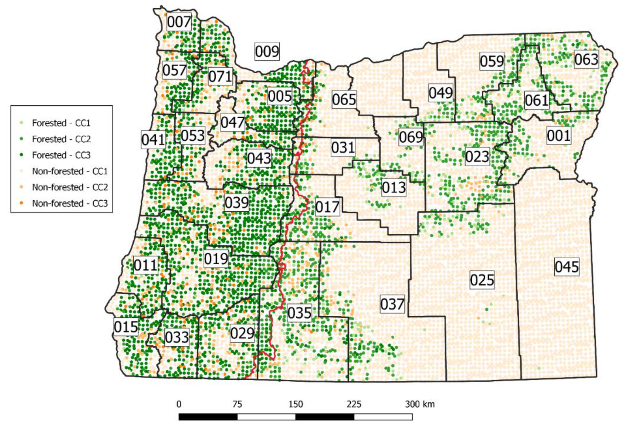
We used a set of 10,537 inventory plots collected by the FIA program between 2009 and 2018. The FIA in Oregon uses a 10-year panel rotation, and this set represents all ten panels, depicted in Figure 1. Each plot is a cluster of four fixed-radius, nested subplots. At each subplot, trees between 12.70 cm and a “breakpoint” diameter are measured on a circular plot of radius 7.32 m and trees larger than the breakpoint diameter are measured on a circular plot of radius 17.95 m. The breakpoint diameter is either 60.96 cm or 76.20 cm depending on whether the plot is east or west of the Cascade Range crest, respectively. For each tree, diameter at breast height (DBH), total height, and species are recorded, among other attributes. Cubic volumes for each tree, including top and stump, are predicted using the National Volume Estimator Library (NVEL) [15].

2.2. Sampling Design, Forest Attributes and Domains

The network of field plot locations for the FIA in Oregon used in this study arise from a random tessellated sampling design [1]. Plot centers were located using a compact hexagonal tessellation with hexagons that are approximately 2184 hectares in size, such that one field plot exists in each hexagon. The plot centers were located using a random azimuth and distance from the hexagon center. In some cases, plots from previous inventory systems were already present, and the locations of those plots were assigned to the hexagon rather than allocating a new field plot. For each field plot we calculated the stem volume ($VOL,{\mathrm{m}}^3{\mathrm{ha}}^{-1}$), basal area ($BA,{\mathrm{m}}^2{\mathrm{ha}}^{-1}$), and stem density ($DEN,{\mathrm{stems}\mathrm{ha}}^{-1}$) for all species combined and for the species that were in the 40th percentile of the total volume in Oregon or greater.

Given this set of 10,537 field plots and their corresponding attributes, we created a population upon which variance estimators could be assessed by assigning each field plot to a position in a discrete two-dimensional space. This discrete space consists of a set of $N=\mathrm{10,537}$ positions upon which systematic sampling can be conducted. Population means of each species-specific attribute considered are given in

Table 1. Population means of the 18 species-specific attributes considered in this study. The proportion of times the species appeared in the $N=\mathrm{10,537}$ field plots is given in the $p_0$ column.

Name	${\mathit{\mu }}_{\mathit{V}\mathit{O}\mathit{L}}$	${\mathit{\mu }}_{\mathit{B}\mathit{A}}$	${\mathit{\mu }}_{\mathit{D}\mathit{E}\mathit{N}}$	${\mathit{p}}_{\mathbf{0}}$
Abies amabilis	2.05	0.22	0.56	0.02
Abies concolor	3.85	0.42	0.82	0.04
Abies grandis	5.05	0.53	1.14	0.07
Abies procera	1.38	0.12	0.18	0.01
Abies shastensis	1.44	0.15	0.20	0.01
Acer macrophyllum	1.77	0.17	0.44	0.04
Alnus rubra	3.13	0.34	0.90	0.05
Arbutus menziesii	1.13	0.14	0.48	0.03
Calocedrus decurrens	1.14	0.16	0.29	0.03
Larix occidentalis	0.94	0.10	0.17	0.03
Picea engelmannii	0.96	0.09	0.16	0.02
Picea sitchensis	1.40	0.12	0.13	0.01
Pinus contorta	2.95	0.45	2.08	0.07
Pinus ponderosa	10.84	1.44	2.84	0.15
Pseudotsuga menziesii	64.59	5.74	8.46	0.28
Thuja plicata	2.43	0.26	0.33	0.04
Tsuga heterophylla	9.51	0.84	1.58	0.08
Tsuga mertensiana	3.36	0.40	0.80	0.02

, along with a proportion representing the number of times the species appeared in a plot divided by $N$.

To subsample this set of $N$ positions, we leveraged the hexagonal tessellation by assigning each field plot to its coincident hexagon in the original sample. The centroids of this set of $N$ hexagons, with forest attributes calculated from the field plots, represents the population upon which systematic sampling is conducted. To retain a hexagonal structure of any systematic sample produced from this population, every $a$th population unit along the horizontal, diagonal, and vertical axes of the hexagonal grid were included in the sample. Let ${\mathit{t}}_{hi}=\left(t_{hi1},t_{hi2}\right)$ represent the row vector of discrete spatial coordinates of the $i$th plot in the $h$th post-stratum. 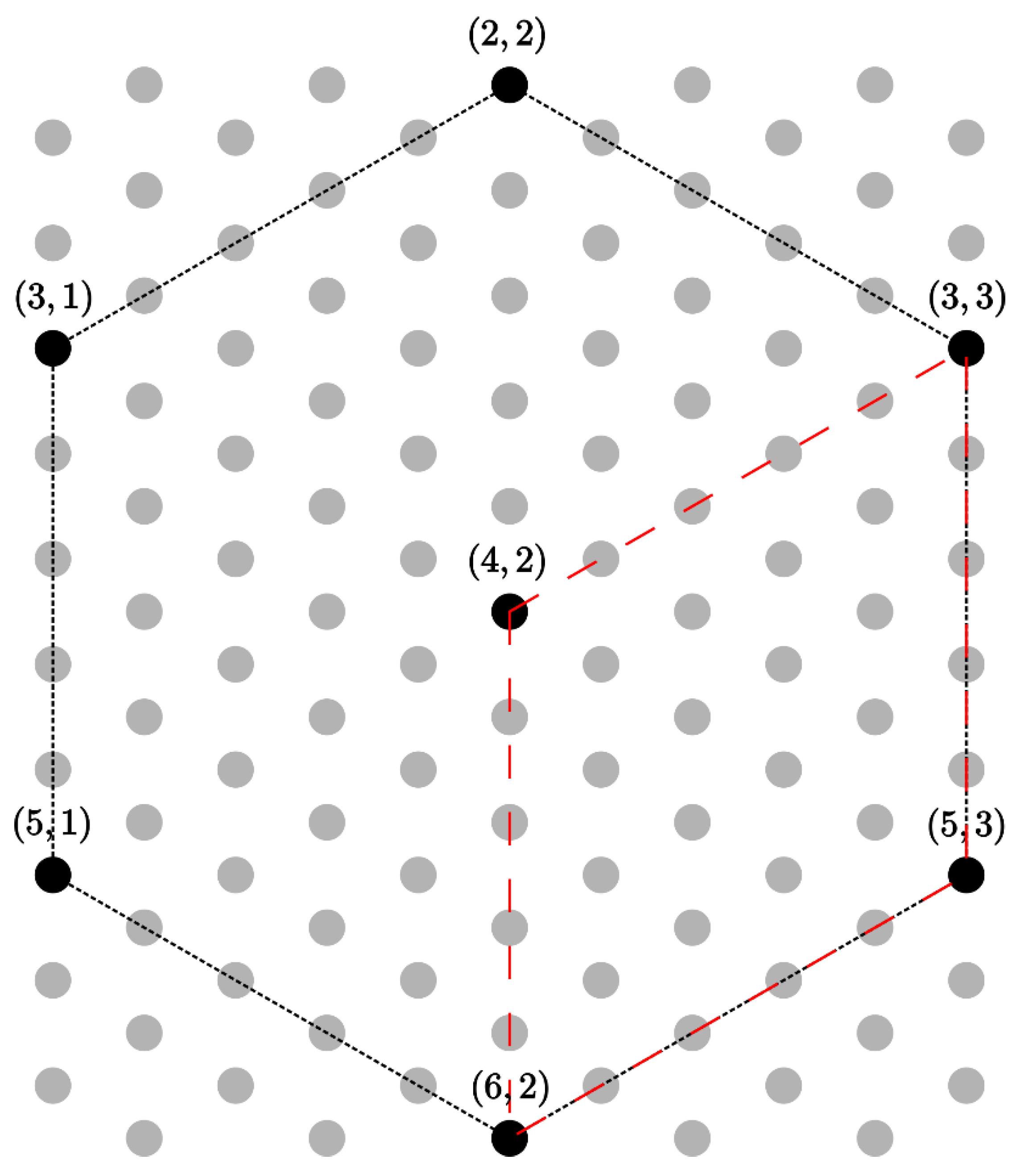Figure 2 displays one possible systematic sample from a hypothetical population in the discrete space with the discrete vectors ${\mathit{t}}_{hi}$ displayed for one systematic sample. Repeating this procedure for every possible systematic sample provides $K=a^2$ samples. We used a sampling interval of $a=5$ for the following assessments. For the remainder of the analysis, the discrete positions ${\mathit{t}}_{hi}$ were treated as the true positions of the field plots.

The performance of the standard estimator of the variance is affected by the degree of spatial correlation between the observations in the sample as well as large-scale trend in a given attribute. By spreading the sample by a distance corresponding to the interval $a$, the spatial correlation will likely decrease, and the observations may become independent. Therefore, the advantage of alternative estimators may not be apparent. However, the density of the sample does not affect trends in the population, and even a less dense sample would allow evaluation of the effect of trends and post-stratification on the performance of the estimators.

The FIA program provides standard reports on many forest attributes for a wide range of domains. Domains are defined as subpopulations of trees that meet certain criteria that serve to define parameters of interest. Examples of domains include spatial domains such as counties, and species domains, such as the set of trees of a particular species. To assess the performance of the estimators when subpopulations are of interest, we defined several domains over which we conducted the analysis: a set of two spatial domains and a set of eighteen species domains. The first spatial domain is the area within the Oregon state boundary, which we will refer to as the “large domain”. In addition to this we create domains from the set of Oregon counties which we refer to as “small domains”. Two adjacent counties (Sherman and Gilliam, east of small domain 65, Figure 1) were removed from consideration as a small domain because no trees were present on any plot. Note that the plots in these counties were still included in the large domain.

The FIA program uses post-strata to enhance the precision of point estimates. FIA uses a large number of post-strata that contain information about forest structure, property ownership, land use and other variables. We used a coarser set of post-strata that mimic the forest structure covariates used operationally by the FIA in Oregon for the purposes of this study. First, we used a forest-non-forest mask produced for 2016 provided by the United States Forest Service Geospatial Technology and Applications Center using the methodology described in [16]. Second, we used three canopy cover classes, corresponding to 0–33%, 33–66% and 66–100% canopy cover derived from a canopy cover map published by the Multi-Resolution Land Characteristics Consortium (http://www.mrlc.gov/ (accessed on 17 August 2020)). Finally, we used an east-west delineation of Oregon derived from the level three ecoregions used by the Environmental Protection Agency (EPA) [17]. The combinations of the forest-non-forest classes, canopy cover classes, and east-west classes produce the twelve post-strata used in this study and are depicted in Figure 1.

2.3. Point Estimators

Observations of plot-level species-specific attributes were calculated by computing a weighted sum of trees that meet the criteria for a given domain. These weights arise from the different sizes used in the nested plot design ([4], p. 53). Let $z\left({\mathit{t}}_{hi}\right)$ represent the observation of the $i$th plot-level forest attribute in the $h$th post-strata at the two-dimensional position vector ${\mathit{t}}_{hi}$. Let $S_k$ refer to the set of index pairs $h$ and $i$ that correspond to the $h$th stratum and $i$th field plot included in the $k$th sample, i.e., each element of $S_k$ is an index pair. We obtain an unbiased estimate of the population mean via the post-stratification estimator under an equal inclusion probability design:

$${\widehat{\mu }}_{PS,k}={{\displaystyle \sum }}_{h=1}^H{W}_h{\overline{z}}_{hk}+\frac{1}{n_k}{{\displaystyle \sum }}_{\left\{h,i\right\} \in S_k}\widehat{e}\left({\mathit{t}}_{hi}\right),$$

(1)

where ${\overline{z}}_{hk}$ is the sample mean of the observations in the $h$th post-stratum, $W_h=\frac{N_h}{N}$ is the weight of the $h$th post-stratum where $N_h$ is the number of population elements in the $h$th post-stratum and $n_k$ is the number of elements in the $k$th sample. This differs from actual practices in the FIA, where $W_h$ is determined from wall-to-wall covariate rasters of fine resolution, rather than field plots [4]. The second summation is over all stratum and plot index pairs in the sample. The error term $\widehat{e}\left({\mathit{t}}_{hi}\right)=z\left({\mathit{t}}_{hi}\right)-{\overline{z}}_{hk}$ explains the deviation of $z\left({\mathit{t}}_{hi}\right)$ from the estimate of the corresponding post-stratum-level mean. Using the above estimator, we can obtain the Horvitz-Thompson estimator for equal inclusion probability designs by setting $H=1$ as a special case. We obtain:

$${\widehat{\mu }}_{HT,k}={\overline{z}}_k+\frac{1}{n_k}{\displaystyle \sum }_{\left\{h,i\right\}\in S_k}\widehat{e}\left({\mathit{t}}_{hi}\right)$$

(2)

where ${\overline{z}}_k$ is the sample mean of the $n_k$ in the sample. Note that the second term is equal to zero and we obtain the sample mean as the HT estimator under equal inclusion probabilities. For brevity, we reserve the notation ${\widehat{\mu }}_k$ to refer to either the HT or PS estimator.

2.4. Variance Estimators

The sampling variance of the PS point estimator under simple random sampling designs is typically approximated using a first order Taylor expansion ([2], p. 235). We obtain:

$$AV\left({\widehat{\mu }}_{PS,k}\right)=fp{c}_k\cdot \frac{1}{n_k\left(N-1\right)}{\displaystyle \sum }_{\left\{h,i\right\}\in U}e{\left({\mathit{t}}_{hi}\right)}^2$$

(3)

where $e\left({\mathit{t}}_{hi}\right)=z\left({\mathit{t}}_{hi}\right)-{\mu }_h$ is the error between $z\left({\mathit{t}}_{hi}\right)$ and its corresponding stratum mean ${\mu }_h$ and $fp{c}_k=\frac{N-n_k}{N}$ is the finite population correction factor for the $k$th sample. Note that, for the HT estimator we obtain $e\left({\mathit{t}}_{hi}\right)=z\left({\mathit{t}}_{hi}\right)-\mu$. Many variance estimators for PS or, more generally, model-assisted estimators consider only this residual term (e.g., [18]). The standard estimator of the systematic variance that assumes the sample was collected with simple random sampling is one such estimator. We obtain the estimator:

$${\widehat{V}}_{SRS}\left({\widehat{\mu }}_k\right)=fp{c}_k\cdot \frac{1}{n_k\left(n_k-1\right)} {{\displaystyle \sum }}_{\left\{h,i\right\}\in S_k}\widehat{e}{\left({\mathit{t}}_{hi}\right)}^2.$$

(4)

In the case of systematic sampling designs, pairwise inclusion probabilities for many population units will be zero, precluding the possibility of unbiased estimation of $AV\left({\widehat{\mu }}_{PS}\right)$. Under HT estimation, many alternatives have been proposed which typically involve squared differences between a local mean of neighboring points and the observation. To make these estimators consistent with PS estimation, we plug in the residual $\widehat{e}\left({\mathit{t}}_{hi}\right)$ to alternative estimators presented for HT variance estimation, which is an approach taken in several other studies [19,20].

Stevens and Olsen [3] proposed a neighborhood-based estimator for the use in the generalized random tessellated stratified (GRTS) sampling design that can be used in systematic designs. The estimator computes a weighted sum of squared errors over the neighborhood $D_{SO,h}\left({\mathit{t}}_{hi}\right)$. The neighborhood is developed iteratively, first by including ${\mathit{t}}_{hi}$ itself plus the $u$ nearest neighbors according to Euclidean distance from the element at ${\mathit{t}}_{hi}$. Then any other points, ${\mathit{t}}_{hj}$, that have ${\mathit{t}}_{hi}$ as a neighbor themselves are added to the neighborhood. Noting that the first-order inclusion probabilities for all units are $a^{-2}$, where $a$ is the systematic sampling interval, we obtain the estimator:

$${\widehat{V}}_{SO,u}\left({\widehat{\mu }}_k\right)=\frac{fp{c}_k}{N^2{a}^4}\cdot {\displaystyle \sum }_{\left\{h, i\right\} \in S_k}{\displaystyle \sum }_{\{h^{\prime },i^{\prime }\} \in D_{SO,u}\left({\mathit{t}}_{hi}\right)}{w}_{hi,h^{\prime }{i}^{\prime }}{\left(\widehat{e}\left({\mathit{t}}_{h^{\prime }{i}^{\prime }}\right)-{\widehat{\overline{e}}}_{D_{SO,u}\left({\mathit{t}}_{hi}\right)}\right)}^2$$

(5)

where $w_{hi,h^{\prime }{i}^{\prime }}$ is a plot-specific weight that decreases as the distance between ${\mathit{t}}_{hi}$ and ${\mathit{t}}_{h^{\prime }{i}^{\prime }}$ increases and ${\widehat{\overline{e}}}_{D_{SO,u}\left({\mathit{t}}_{hi}\right)}={\displaystyle \sum }{w}_{hi,h^{\prime }{i}^{\prime }}\widehat{e}\left({\mathit{t}}_{h^{\prime }{i}^{\prime } }\right)$. This distance weighting effect is similar to kriging, where residual pairs that are close together will be weighted more than pairs of residuals further away when computing the neighborhood-level variance. These weights are optimized by ensuring the sum of ${\widehat{\overline{e}}}_{D_{SO,u}\left({\mathit{t}}_{hi}\right)}$ over all plots adds up to the total error (refer to [3] for further information on this optimization procedure). We consider the special case where $u=12$. Implementations for ${\widehat{V}}_{SO}$ were provided by the R package spsurvey [21].

Matérn ([11], pp. 120–122) describes an estimator for two-dimensional systematic sampling designs that relies on computing contrasts of units within non-overlapping neighborhoods as local variance estimates and aggregating these variance estimates over all neighborhoods to produce a final estimate. We considered two neighborhood configurations. First, we consider:

$$D_{MAT,hex}\left({\mathit{t}}_{hi}\right)=\left\{\left(t_{hi1}-1, t_{hi2}-1\right), \left(t_{hi1}, t_{hi2}-2\right),\left(t_{hi1}-1, t_{hi2}+1\right),\left(t_{hi1}-1, t_{hi2}+1\right),\left(t_{hi1},t_{hi2}+2\right),\left(t_{hi1}+1, t_{hi2}+1\right)\right\}$$

(6)

which represents the nearest neighbors with respect to ${\mathit{t}}_{hi}$ and:

$$D_{MAT,par}\left({\mathit{t}}_{hi}\right)=\left\{\left(t_{hi1},t_{hi2}\right), \left(t_{hi1}-1,t_{hi2}+1\right),\left(t_{hi1}+1,t_{hi2}+1\right), \left(t_{hi1},t_{hi2}+2\right)\right\}$$

(7)

which represents a parallelogram constructed from the neighbors of ${\mathit{t}}_{hi}$ and itself. This second configuration closely mimics the original Matérn estimator, which was developed for the case of rectangular grids. Both neighborhood specifications are displayed in Figure 2.

For each neighborhood, a contrast of the mean-centered residuals of the elements in the neighborhood is computed. Let ${\widehat{\mathit{e}}}_{ct,l}={\left({\widehat{e}}_{hi}\left({\mathit{t}}_{h^{\prime }{i}^{\prime }}\right)-{\widehat{\overline{e}}}_{D_{MAT,c}\left({\mathit{t}}_{hi}\right)}\right)}^T, \{h^{\prime }{i}^{\prime }\}\in D_{MAT,c}\left({\mathit{t}}_{hi}\right)$ represent the vector of mean-centered residuals for the $l$th neighborhood using configuration $c$ of the Matérn estimator (

Table 2. Notation, name, and configurations of the variance estimators used in this study. A canonical study that uses the estimator is included if available.

Notation	Name	Configurations	Reference
${\widehat{V}}_{SRS}$	Simple random sampling estimator	--	--
${\widehat{V}}_{SO,h}$	Stevens and Olsen estimator	$u\in \left\{12\right\}$—number of nearest neighbors	[3]
${\widehat{V}}_{MAT,c}$	Matern estimator	$c\in \left\{hex, par\right\}$—neighborhood contrast structure	[11]
${\widehat{V}}_{DC,o}$	D’Orazio (2003)–Geary’s C	$o\in \left\{1,2\right\}$—neighborhood order	[12]

). Points in the neighborhood that fall outside of the study space are given a value of zero. For each neighborhood calculate the value:

$$T_l=\frac{{\left({\widehat{\mathit{e}}}_{ct,l}^T{\mathit{c}}_l\right)}^2}{n_l}$$

(8)

where $n_l$ indicates the number of sampled population units in the neighborhood and ${\mathit{c}}_l$ is a vector containing elements that are either −1 or 1. We use the vectors ${\left(1, 1, 1,-1,-1,-1\right)}^T$ and ${\left(1,1,-1-1\right)}^T$ for the hexagonal and parallelogram neighborhood structures, respectively. The positive and negative elements of ${\mathit{c}}_l$ create two groups which each make a prediction for the mean residual in the neighborhood, and Equation (8) calculates a squared difference between these two predictions. This squared difference creates the basis for a neighborhood-level variance estimate. Using these values, we obtain the Matérn variance estimator:

$${\widehat{V}}_{MAT,c}\left({\widehat{\mu }}_k\right)=fp{c}_k\cdot \frac{q_c}{n^2}{\displaystyle \sum }_{l=1}^L{T}_l$$

(9)

where $q_{par}=4$ and $q_{hex}=7$ for the parallelogram and hexagonal neighborhood structures, respectively.

Adjustment-based estimators rely on applying an adjustment factor to ${\widehat{V}}_{SRS}$ that approximates the inter-cluster correlation coefficient. This approach is motivated by the fact that variance estimates using ${\widehat{V}}_{SRS}$ in the case of systematic sampling will tend to have a larger positive bias in situations where the inter-cluster correlation, i.e., the correlation between pairs of possible systematic samples, is strongly positive or negative. One such estimator was proposed by D’Orazio [12] which relies on the Geary’s C index. We consider two neighborhood structures. The first structure considers the six closest points to an element at ${\mathit{t}}_{hi}$ to be neighbors. 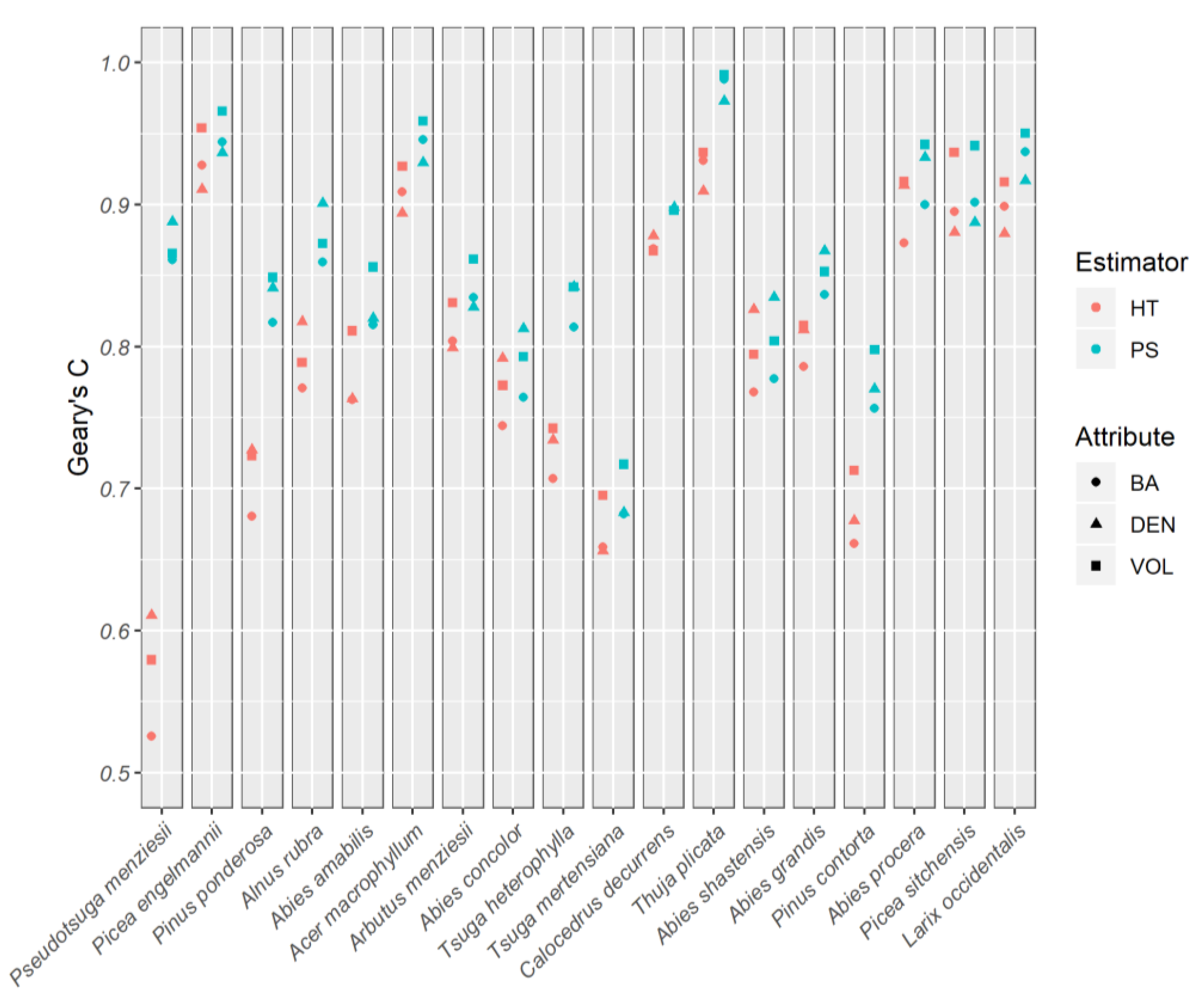This is equivalent to the $D_{MAT,hex}$ neighborhood. We also consider second order neighbors, i.e., those elements that are first order neighbors, as well as their first order neighbors. Noting this we obtain the expression for Geary’s C:

$$C_k=\frac{\left(n_k-1\right){{\displaystyle \sum }}_{hi}{{\displaystyle \sum }}_{h^{\prime }{i}^{\prime }}{\delta }_{hi,h^{\prime }{i}^{\prime }}{\left(\widehat{e}\left({\mathit{t}}_{hi}\right)-\widehat{e}\left({\mathit{t}}_{h^{\prime }{i}^{\prime }}\right)\right)}^2}{2\left({{\displaystyle \sum }}_{hi}{{\displaystyle \sum }}_{h^{\prime }{i}^{\prime }}{\delta }_{hi,h^{\prime }{i}^{\prime }}\right)\left({{\displaystyle \sum }}_{hi}\widehat{e}{\left({\mathit{t}}_{hi}\right)}^2\right)}$$

(10)

where ${\delta }_{hi,h^{\prime }{i}^{\prime }}$ is an indicator variable that takes the value one if the element at ${\mathit{t}}_{hi}$ is considered a neighbor of the element at ${\mathit{t}}_{h^{\prime }{i}^{\prime }}$. We obtain the D’Orazio’s Geary’s C estimator:

$${\widehat{V}}_{DC}\left({\widehat{\mu }}_k\right)=\{\begin{array}{l}{\widehat{V}}_{SRS}\left({\widehat{\mu }}_k\right)\cdot C_k, \hspace{1em}{\displaystyle \sum }_{hi}\widehat{e}{\left({\mathit{t}}_{hi}\right)}^2\ne 0\\ \hspace{1em}\hspace{0.17em}{\widehat{V}}_{SRS}\left({\widehat{\mu }}_k\right),\hspace{1em}\hspace{1em}o.w.\end{array}.$$

(11)

The first condition of (11) ensures that Geary’s C can be calculated. If not, ${\widehat{V}}_{SRS}$ is used without adjustment. For the purposes of reporting results, we calculate Geary’s C using Equation (10) with all $N$ field plots using the residuals obtained from the HT estimator. We refer to this quantity as $C$ for the remainder of the text.

2.5. Performance Measures

Define a systematic sampling interval $a$ such that every $a$th element along each axis is sampled. Sampling in this fashion for a hexagonal tessellation implies that there are $a^2=K$ possible subsamples. Furthermore, all samples produced will retain a hexagonal structure (Figure 2). Using all subsamples, we obtain the actual variance of the estimator, which we will refer to as the “true variance” for brevity:

$$V_{SYS}\left({\widehat{\mu }}^{\left(p\right)}\right)=\frac{1}{K}{\displaystyle \sum }_{k=1}^K{\left({\mu }^{\left(p\right)}-{\widehat{\mu }}_k^{\left(p\right)}\right)}^2$$

(12)

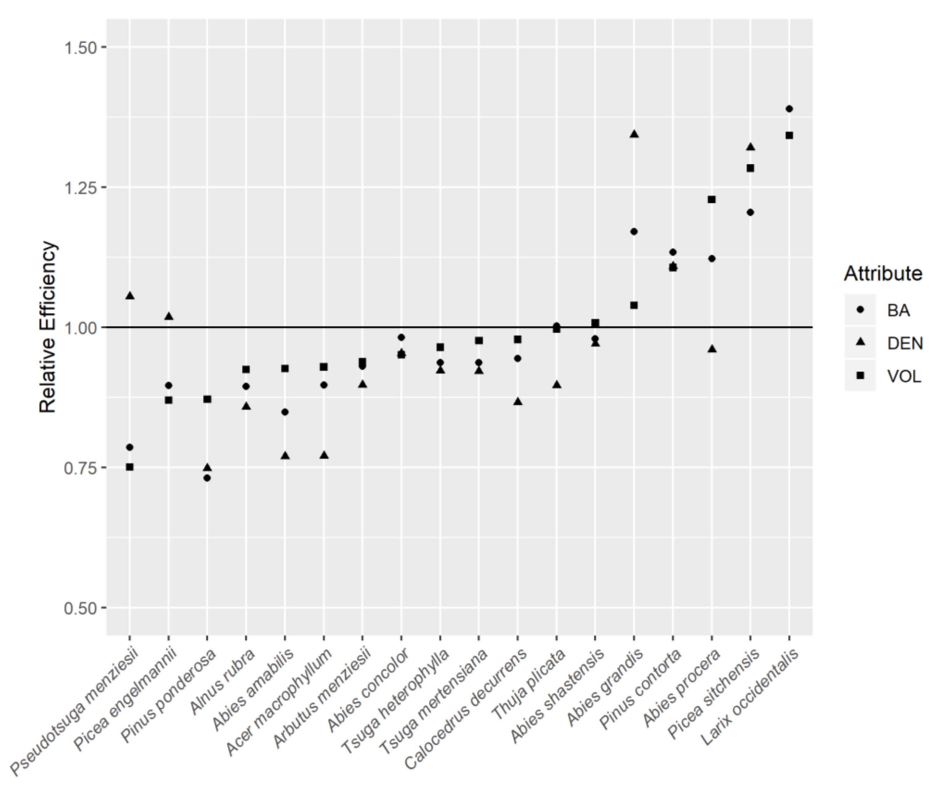
where the superscript $\left(p\right)$ is used to refer to a domain-attribute combination indexed by $p$. Although secondary to the objective of this study, comparing the performances of the point estimators HT and PS can be done using the relative efficiency of the true variances:

$$RE\left({\widehat{\mu }}_{HT}^{\left(p\right)},{\widehat{\mu }}_{PS}^{\left(p\right)}\right)=\frac{V_{SYS}\left({\widehat{\mu }}_{HT}^{\left(p\right)}\right)}{V_{SYS}\left({\widehat{\mu }}_{PS}^{\left(p\right)}\right)}.$$

(13)

We relied on two general categories of performance measures to assess the behavior of the proposed variance estimators. The first category assesses the performance of an estimator for a particular attribute in a particular domain. Let ${\widehat{V}}_{gk}^{\left(p\right)}$ refer to the $k$th variance estimate for the $p$th domain-attribute combination for estimator $g\in \left\{IRS, SO, \dots , DI,2\right\}$. For brevity, let $V_{SYS}\left({\widehat{\mu }}^{\left(p\right)}\right)=V_{SYS}^{\left(p\right)}$. 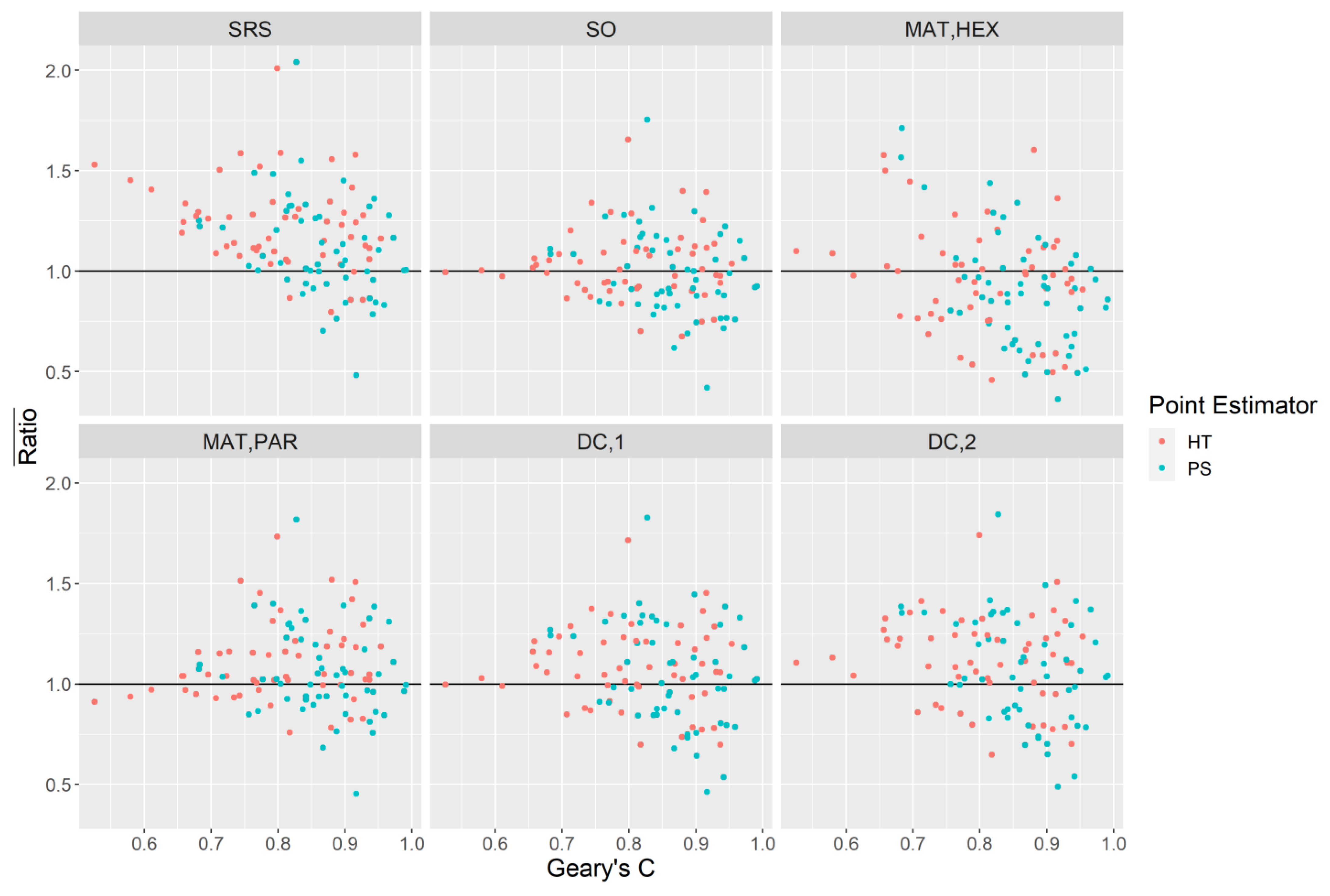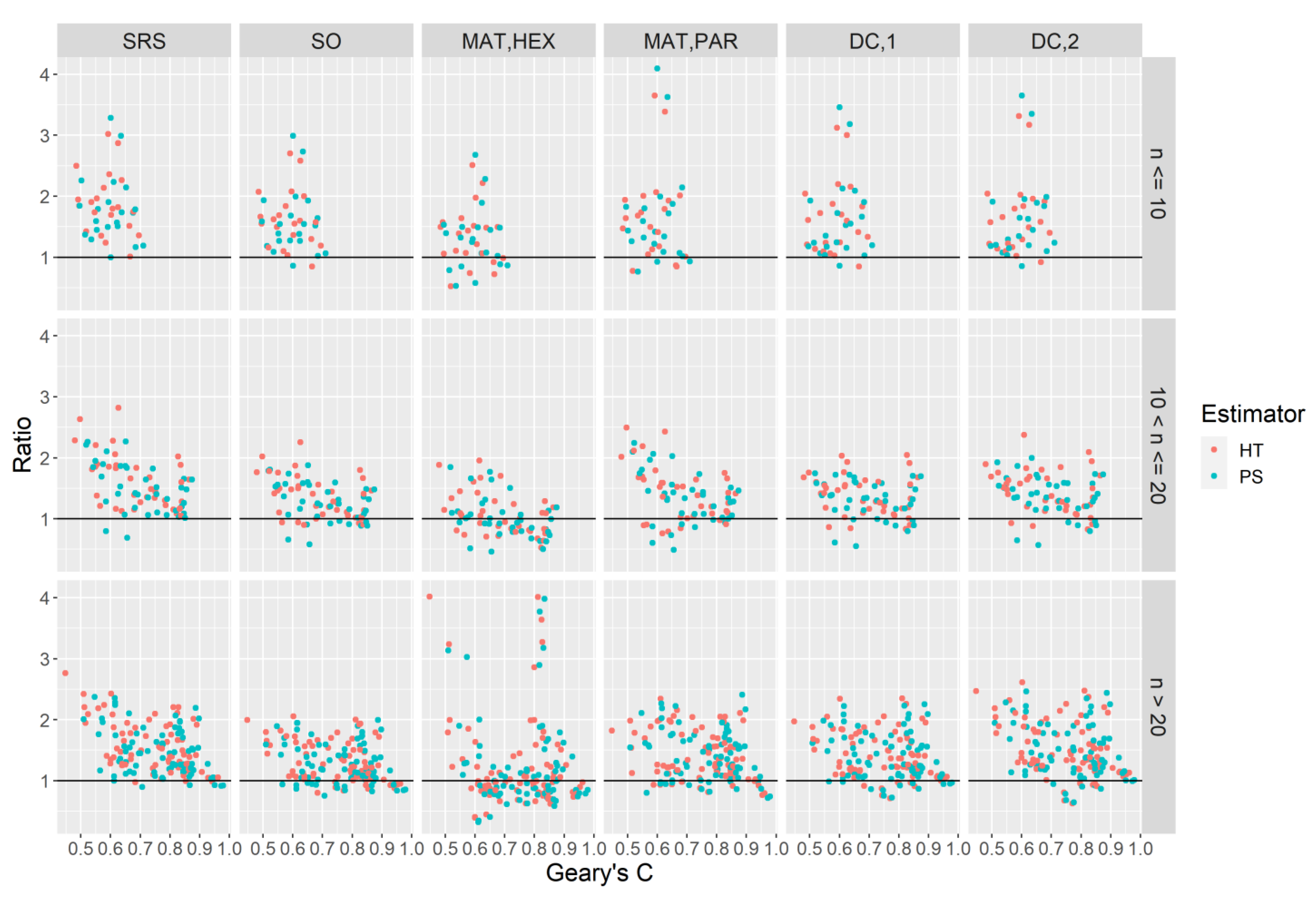We obtain the mean error of the ratio of the variance estimate to the systematic variance:

$$\overline{Ratio}\left({\widehat{V}}_k^{\left(p\right)}\right)=\frac{1}{K}{\displaystyle \sum }_{k=1}^K\frac{{\widehat{V}}_{gk}^{\left(p\right)}}{V_{SYS}^{\left(p\right)}}$$

(14)

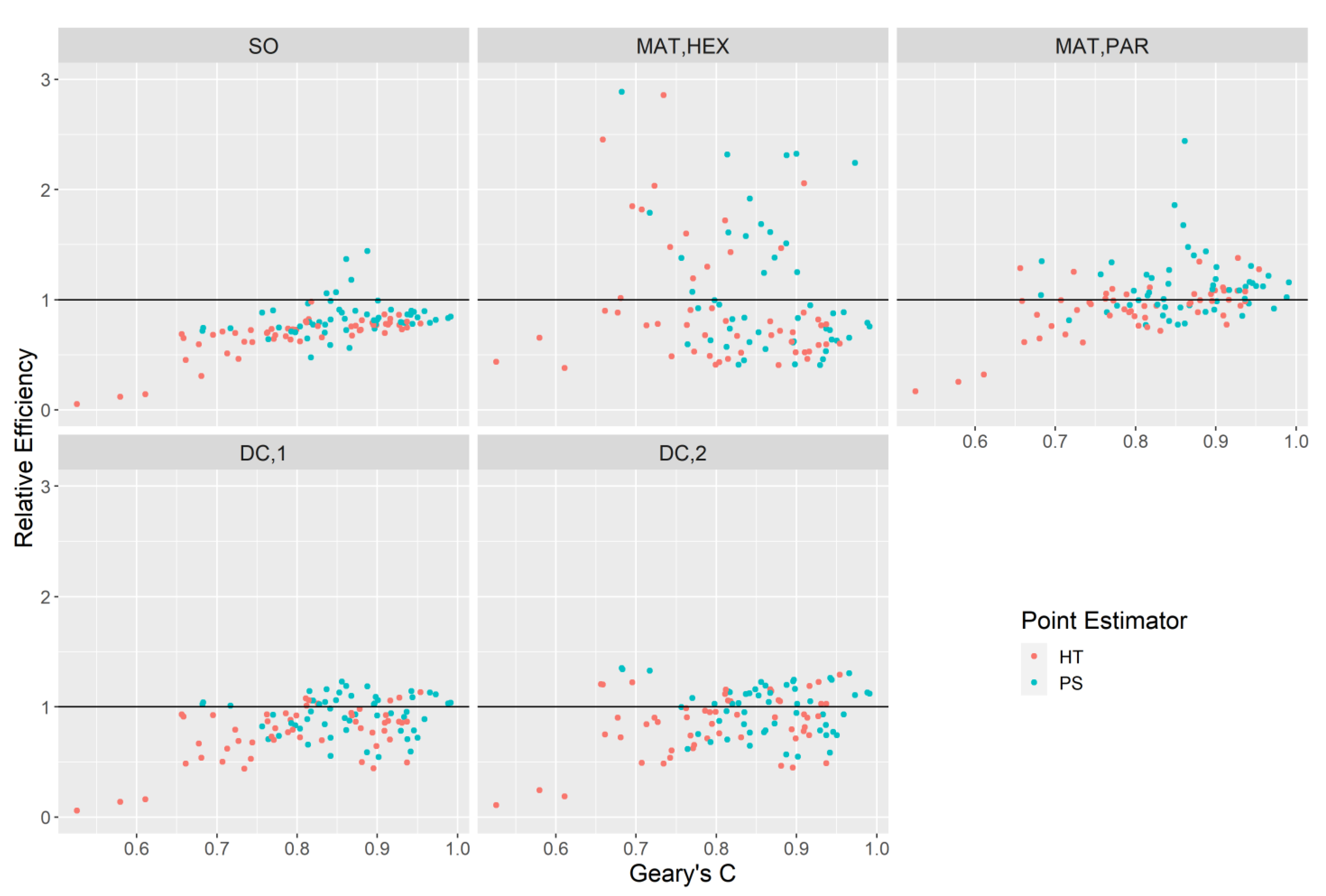
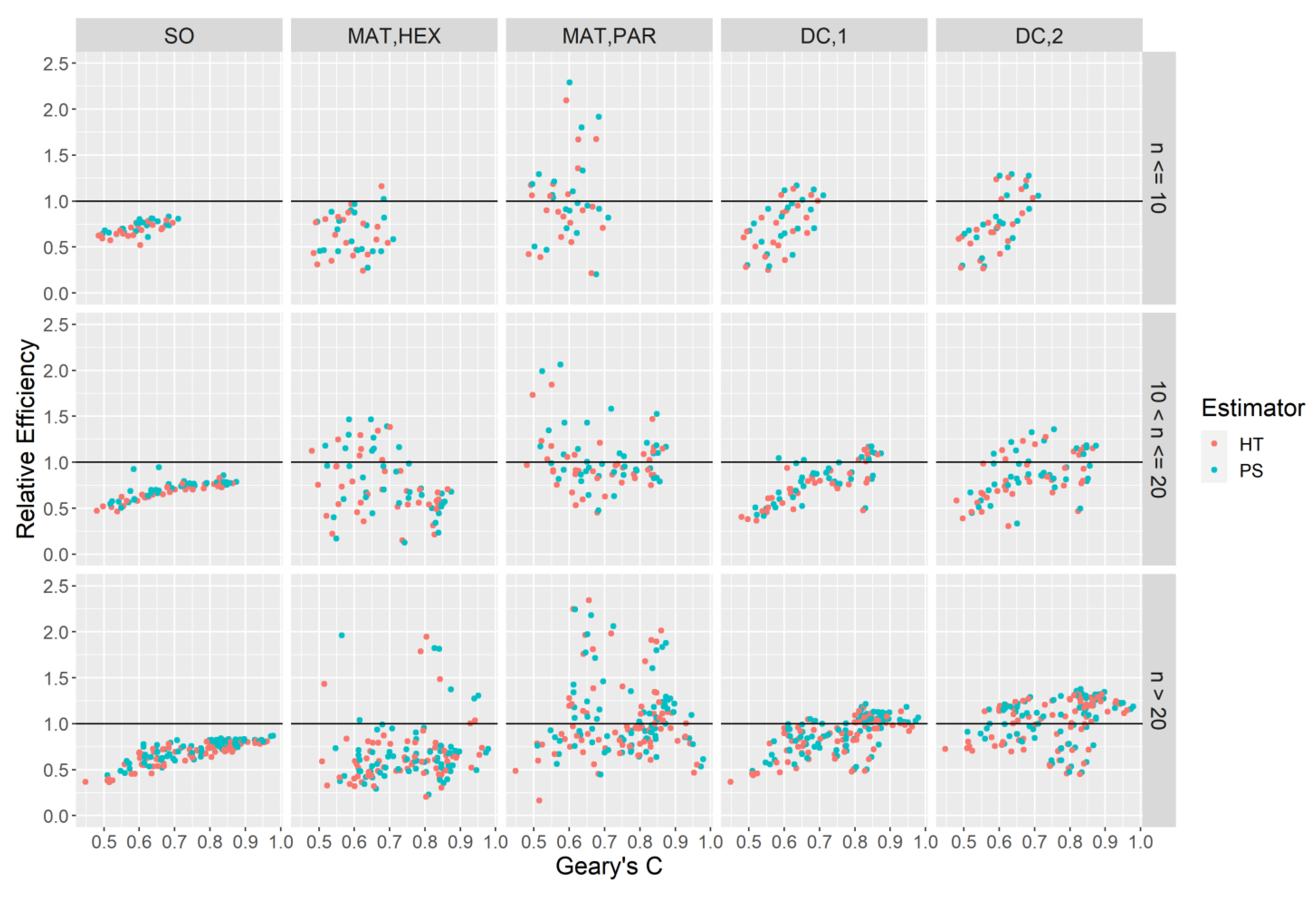
which quantifies the mean deviation of the ratio of the variance estimate from one. $\overline{Ratio}\left({\widehat{V}}_k^{\left(p\right)}\right)$ is equivalent to the design expectation of the quantity $\frac{{\widehat{V}}_{gk}^{\left(p\right)}}{V_{SYS}^{\left(p\right)}}$. Equation (14) can be considered a relative measure of bias for a variance estimate for a particular domain-attribute combination. In addition to (14) we also produce the relative efficiencies of the variance estimators themselves with respect to the simple random sampling estimator, ${\widehat{V}}_{SRS}$. In many environmental sampling surveys ${\widehat{V}}_{SRS}$ is considered the standard choice for a variance estimator under this design and thus assessing the alternatives with respect to ${\widehat{V}}_{SRS}$ can provide valuable information on potential efficiency gains. We obtain:

$$RE\left({\widehat{V}}_{g^{*}}^{\left(p\right)}, {\widehat{V}}_{SRS}^{\left(p\right)}\right)=\frac{SSE\left({\widehat{V}}_{g^{*}}^{\left(p\right)}\right)}{SSE\left({\widehat{V}}_{SRS}^{\left(p\right)}\right)}$$

(15)

where $g^{*}$ represents any estimator that is not the simple random sampling estimator and $SSE\left({\widehat{V}}_g^{\left(p\right)}\right)={\displaystyle \sum }_{k=1}^K{\left({\widehat{V}}_g^{\left(p\right)}-V_{SYS}^{\left(p\right)}\right)}^2$ is the sum of squared errors for a given estimator over all $K$ subsamples.

The second category of performance measures consider the performance of an estimator across several domain-attribute combinations. We consider the mean of the mean ratio across all $p$ domain-attribute combinations:

$$\overline{\overline{Ratio}}\left({\widehat{V}}_g\right)=\frac{1}{P}{\displaystyle \sum }_{p=1}^P\overline{Ratio}\left({\widehat{V}}_g^{\left(p\right)}\right).$$

(16)

while $\overline{Ratio}$ is a measure of relative bias, $\overline{\overline{Ratio}}$ is simply an aggregation of these measures across several attributes and is not strictly a measure of bias itself. Instead, $\overline{\overline{Ratio}}$ can be interpreted as a performance index over many estimates of the true variance for a particular estimator. $\overline{\overline{Ratio}}$ values close to one indicate a tendency for an estimator to over-estimate the true variance across many domain-attribute combinations, and vice versa. In a similar manner, we consider the mean of the relative efficiencies across all $P$ domain-attribute combinations and obtain:

$$\overline{RE}\left({\widehat{V}}_g\right)=\frac{1}{P} {\displaystyle \sum }_{p=1}^{P}RE\left({\widehat{V}}_g^{\left(p\right)}\right)$$

(17)

which is the mean relative efficiency for a given estimator over all $P$ domain-attribute combinations.

3. Results

3.1. Comparison of Point Estimators

We estimated three attributes (VOL, BA, and DEN) for each species considered in this analysis using the PS estimator and HT estimator. The relative efficiencies of these point estimators for each species-specific attribute are shown in Figure 3. For most species-specific attributes, the use of the post-stratification estimator provides a lower variance (i.e., a relative efficiency less than one) than the Horvitz-Thompson estimator, with relative efficiencies as low as 0.75 for the VOL attribute of Pseudotsuga menziesii. In some cases, the post-stratified estimator was not as efficient, e.g., for Abies grandis and Pinus contorta, among others, with relative efficiencies as high as 1.4. This suggests that the post-strata correlate well with species-specific attributes for some species, but not others. Note that species with larger relative efficiencies tended to have a much lower prevalence (Table 1). Additionally, we used a much coarser set of post-strata than is used in official reporting by the FIA, and relative efficiencies using this larger set of post-strata may be lower than what we obtained.

The HT and PS point estimators imply different correlation structures among the residuals attained in Equations (1) and (2) for the same species-specific attributes, as well as different models for the trend. We summarize changes in this structure using the Geary’s C correlation coefficient, $C$, in Figure 4. For all species-specific attributes we considered, $C$ increased when going from the HT to the PS estimator. The effect is most extreme for Pseudotsuga menziesii and Pinus ponderosa attributes. A large change in $C$ implies that the post-stratification variables explain either the linear trend or the spatial correlation structure of the residuals more than without (i.e., under HT estimation). Even under the PS estimator, however, $C$ remains large, implying that some spatial dependence is present in the residual, or that the post-stratification variables do not completely accommodate the trend, or both. Large increases in $C$ are present for Pseudotsuga menziesii, Pinus ponderosa, and Alnus rubra for all three attributes. Other species exhibited only moderate increases.

3.2. Comparison of Variance Estimators

3.2.1. Large Spatial Domain Assessment

For the large domain assessment, we produced variance estimators and their performance measures considering species-specific attributes. Figure 5 displays the $\overline{Ratio}$ for species-specific attributes for all variance estimators under HT and PS point estimation. For ${\widehat{V}}_{SRS}$ under the HT point estimator the degree of positive bias for attributes with small $C$ values (i.e., stronger spatial dependence) is large. As this spatial dependence weakens, the degree of bias becomes less apparent. Under the PS point estimator, the range of $C$ values decreases (Section 3.1) and the positive bias of ${\widehat{V}}_{SRS}$ is reduced to some degree. For the alternative estimators under the HT estimator the positive bias observed for ${\widehat{V}}_{SRS}$ for small $C$ attributes is clearly reduced, producing ratio estimates very close to one. For attributes with $C$ values exceeding 0.7 this reduction is not as clear.

Figure 6 displays the relative efficiency for each of the $P$ domain-attribute combinations under the HT and PS point estimators. Generally, the alternative estimators improve over ${\widehat{V}}_{SRS}$, as indicated by the points that fall below the solid line. Under HT estimation this improvement is most clear for domain-attribute combinations with small $C$ values. Under the PS point estimator, the improvement is not as clear, with several notable points falling above the solid line. The ${\widehat{V}}_{SO}$, ${\widehat{V}}_{DC,1}$, and ${\widehat{V}}_{DC,2}$ estimators appear to have the most reliable improvements under both HT and PS point estimators, with only relatively few points falling above the solid line.

Table 3. Performance summaries of all variance estimators for the large spatial domain under HT and PS estimation.

Variance Estimator	Point Estimator	$\overline{\overline{\mathit{R}\mathit{a}\mathit{t}\mathit{i}\mathit{o}}}$	$\overline{\mathit{R}\mathit{E}}$
${\widehat{V}}_{SRS}$	HT	1.23	--
	PS	1.11	--
${\widehat{V}}_{SO}$	HT	1.01	0.65
	PS	0.96	0.82
${\widehat{V}}_{MAT,hex}$	HT	0.96	1.16
	PS	0.90	1.51
${\widehat{V}}_{MAT,par}$	HT	1.10	0.92
	PS	1.06	1.12
${\widehat{V}}_{DC,1}$	HT	1.08	0.77
	PS	1.05	0.93
${\widehat{V}}_{DC,2}$	HT	1.12	0.84
	PS	1.07	0.99

summarizes the estimators across the $P$ domain-attribute combinations. Under HT estimation the ${\widehat{V}}_{SRS}$ tended to demonstrate positive bias, with a $\overline{\overline{Ratio}}$ value of 1.23. The positive bias for the alternative estimators under HT estimation is less, with $\overline{\overline{Ratio}}$ values ranging between 0.96 to 1.12. The relative efficiencies for the alternative estimators were less than one except for ${\widehat{V}}_{MAT,par}$, which suggests that these alternatives provide gains in efficiency under the HT estimator. Under the PS point estimator, the ${\widehat{V}}_{SRS}$ estimator demonstrates positive bias with a $\overline{\overline{Ratio}}$ value of 1.11. The alternative estimators had smaller $\overline{\overline{Ratio}}$ values, ranging between 0.90 to 1.08. The mean relative efficiencies under the PS point estimators were less than one with the exception of ${\widehat{V}}_{MAT,par}$ and ${\widehat{V}}_{MAT,hex}$, although these relative efficiencies are slightly higher than the analogous estimators under the HT point estimator.

3.2.2. Small Spatial Domain Assessment

In addition to the large spatial domain, we conducted an assessment for the species-specific attributes for the small domains in Oregon that correspond, in most cases, to existing county boundaries (see Section 2.2). Such an assessment provides a range of different, albeit smaller, populations, each with $P$ domain-attribute combinations exhibiting a range of spatial structures. If a species-specific attribute had an estimate of zero for any of the $K$ subsamples within a domain, then the species-specific attribute was discarded for that domain. This was considered appropriate because a desirable property for a variance estimator is to produce a variance of zero if there is no variance between sample observations. However, this property guarantees a given estimator will be negatively biased in the case where the point estimate is zero. For this reason, species-specific attributes within a domain are removed from consideration if any point estimate for that domain was zero among the $K$ subsamples. In total, there are 30 small domains that contain between six to 30 species-specific attributes. For each small domain, the sample size within that domain is a random variable. Let $n_c^{\prime }$ represent the mean sample size across the $K$ subsamples within a small domain. We assign each domain to one of three classes, based on its sample size: $n_c^{\prime }\le 10$, $10<n_c^{\prime }\le 20$ and $n_c^{\prime }>20$. These thresholds represent the 33rd and 66th percentile of the domain-specific sample sizes across study areas.

We produced variance estimates for each of these species-specific attributes in each small domain under the HT and PS estimators (Figure 7). Generally, all estimators exhibited a strong positive bias across the range of $C$ values and across all sample size classes, with a diminishing positive bias as the sample size increased. For most estimators, variance estimation under the post-stratified estimator reduced the bias with notable exceptions for some of the attributes in the smallest sample size classes. In the small sample size classes, two specific attributes are apparent as positive outliers for all estimators that correspond to the VOL and BA attribute in spatial domain 47 (see Figure 1). However, these outliers have $\overline{Ratio}$ values that are more extreme than the ${\widehat{V}}_{SRS}$ estimator for the ${\widehat{V}}_{DC,1}$, ${\widehat{V}}_{DC,2}$ and ${\widehat{V}}_{MAT,par}$ estimators.

All three of these alternative estimators rely to some extent on the definition of neighborhoods surrounding given sample positions (Equations (5), (6) and (9)). For a small spatial domain, these estimators will only have access to relatively few neighborhoods to compute the variance, which may lead to the extreme values we observe. In addition, spatial domain 47 appears to have a large perimeter-to-area ratio and is very irregular in shape. In contrast, ${\widehat{V}}_{SO}$ constructs neighborhoods for each point in the sample space, which provides a larger number of neighborhoods used to estimate the variance, which may resolve some of these issues.

Generally, the estimators attain lower relative efficiencies as sample size increases (Figure 8) with notable exceptions occurring for the ${\widehat{V}}_{MAT,par}$ estimator. The ${\widehat{V}}_{SO}$ estimator is more efficient the ${\widehat{V}}_{SRS}$ across all of the possible attributes, and ${\widehat{V}}_{DC,1}$ is more efficient for many, but not all, attributes. Only small differences exist between variance estimates attained under HT or PS point estimators. Generally, variance estimates attained under PS point estimation have slightly higher relative efficiencies, suggesting that the PS point estimator removes some of the benefit of using an alternative estimator.

The SRS variance estimator has the largest $\overline{\overline{Ratio}}$ value among all estimators considered across all three sample size classes with the exception of ${\widehat{V}}_{DC,2}$ under the post-stratified estimator (

Table 4. $\overline{\overline{Ratio}}$ and $\overline{RE}$ disaggregated by the small domain sample size class for all estimators under the HT and PS estimators.

Variance Estimator	Point Estimator	$\overline{\overline{\mathit{R}\mathit{a}\mathit{t}\mathit{i}\mathit{o}}}$			$\overline{\mathit{R}\mathit{E}}$
		${\mathit{n}}_{\mathit{c}}^{\mathbf{\prime }}\mathbf{\le }\mathbf{10}$	$\mathbf{10}\mathbf{<}{\mathit{n}}_{\mathit{c}}^{\mathbf{\prime }}\mathbf{\le }\mathbf{20}$	${\mathit{n}}_{\mathit{c}}^{\prime }>20$	${\mathit{n}}_{\mathit{c}}^{\prime }\le 10$	$10<{\mathit{n}}_{\mathit{c}}^{\prime }\le 20$	${\mathit{n}}_{\mathit{c}}^{\prime }>20$
${\widehat{V}}_{SRS}$	HT	1.88	1.63	1.54	--	--	--
	PS	1.78	1.48	1.47	--	--	--
${\widehat{V}}_{SO}$	HT	1.62	1.36	1.31	0.68	0.67	0.68
	PS	1.57	1.27	1.27	0.73	0.72	0.72
${\widehat{V}}_{MAT,hex}$	HT	1.34	1.07	1.24	0.79	0.71	1.28
	PS	1.30	1.00	1.21	0.85	0.78	1.39
${\widehat{V}}_{MAT,par}$	HT	1.67	1.41	1.42	0.97	0.97	1.03
	PS	1.64	1.32	1.40	1.06	1.06	1.07
${\widehat{V}}_{DC,1}$	HT	1.64	1.39	1.42	0.71	0.74	0.85
	PS	1.60	1.30	1.39	0.77	0.81	0.90
${\widehat{V}}_{DC,2}$	HT	1.66	1.45	1.52	0.74	0.83	1.01
	PS	1.62	1.36	1.48	0.79	0.89	1.05

). The ${\widehat{V}}_{SRS}$ estimator under post-stratification has a lower $\overline{\overline{Ratio}}$ value than under the HT estimator, which is consistent with the large domain assessment in Section 3.2.1. The ${\widehat{V}}_{MAT,hex}$ estimator attained the $\overline{\overline{Ratio}}$ value closest to zero under both the HT and PS point estimators. With the exception of the ${\widehat{V}}_{MAT,par}$ estimator, all alternative estimators attained a lower mean relative efficiency, with the ${\widehat{V}}_{SO}$ estimator attaining the lowest relative efficiency across all three sample size classes ranging between 0.67 and 0.68 relative efficiency.

4. Discussion

4.1. Variance Estimation under Horvitz-Thompson and Post-Stratification Estimators

We examined performance measures for six variance estimators under HT and PS point estimation for a variety of populations and spatial domains. Considering both HT and PS estimation provides insight into how well the variance estimators can handle populations with varying spatial structure in the residual. A robust variance estimator should be able to handle these diverse situations under both point estimation regimes.

Several studies have examined variance estimation for systematic and similar designs under a Horvitz-Thompson point estimator. Magnussen et al. [6] investigated alternative variance estimators under simulated populations and found improvements for estimators similar to ${\widehat{V}}_{DC,1}$ and ${\widehat{V}}_{MAT,par}$ with $\overline{\overline{Ratio}}$ values ranging between 1.03 to 1.37 and 0.98 to 1.19, respectively while attaining ${\widehat{V}}_{SRS}$ values ranging between 1.50 to 2.88. Similarly, Stevens and Olsen [3] present results using ${\widehat{V}}_{SO}$ under a generalized random tessellated stratified design and attained $\overline{Ratio}$ close to one and confidence interval coverage probabilities very close to the nominal rate using a simulated data set. Our results also indicate improvements using the alternative estimators. For the large spatial domain, we noted a trend of positive bias for the ${\widehat{V}}_{SRS}$ estimator with decreasing Geary’s C (Figure 5 and Figure 7). Specifically, we attained $\overline{\overline{Ratio}}$ values of 1.23 for the large domain and values between 1.54 to 1.88 for the small spatial domains. Several alternative estimators provide clear improvements over ${\widehat{V}}_{SRS}$ under an HT point estimator. ${\widehat{V}}_{SO}$ and ${\widehat{V}}_{DC,1}$ attained $\overline{\overline{Ratio}}$ values closer to one and smaller relative efficiencies in both the large spatial domain and small spatial domains. Notably, ${\widehat{V}}_{SO}$ was the only estimator that attained smaller relative efficiencies for every species-specific attribute we considered across all spatial domains under the HT point estimator (Figure 7 and Figure 8).

When moving from HT to PS point estimation, two things may happen; a reduction in the spatial dependence in the residual and removal of at least some of the large-scale trend. Both of these can reduce the positive bias of the ${\widehat{V}}_{SRS}$ [6,22]. We found a reduction in $C$ for the residuals (Figure 4), and an increase in relative efficiency of the point estimates for many attributes (Figure 3) when moving from HT to PS, suggesting that the removal of some spatial correlation and some trend is expected for these attributes. However, for many species-specific attributes this change was small. This implies that the positive bias typically observed under the ${\widehat{V}}_{SRS}$ estimator may remain even under PS point estimation for the attributes and post-strata we considered (Table 3 and Table 4), motivating the adoption, or at least consideration, of the alternative estimators we present. While it is possible to reduce this bias with higher quality covariates (e.g., [23]), covariates that correlate well with species-specific attributes may not be available. Note that the FIA uses a more detailed stratification, exceeding 100 different strata for the state of Oregon, and may provide lower relative efficiencies under PS estimation than we observed. For the large spatial domain we attained $\overline{\overline{Ratio}}$ close to one under the PS point estimator with values of 0.96 and 1.05 for the ${\widehat{V}}_{SO}$ and ${\widehat{V}}_{DC,1}$ estimators respectively (Table 3). All alternative estimators showed improvements for the small spatial domains across all sample size classes, i.e., they attained $\overline{\overline{RE}}$ lower than one and $\overline{\overline{Ratio}}$ closer to one than the ${\widehat{V}}_{SRS}$ estimator (Table 4).

Some of the estimators appear to have a large number of outlier points, e.g., the ${\widehat{V}}_{MAT,hex}$ and ${\widehat{V}}_{MAT,par}$ estimators (Figure 7). Closer inspection of the spatial domains where these outliers manifested revealed very sparse populations, i.e., with many observations of attributes that are zero. The ${\widehat{V}}_{MAT}$ estimators rely on a much smaller number of neighborhoods to compute a variance estimate relative to ${\widehat{V}}_{SO}$ and in populations that have widely varying neighborhood-level estimates of variance, this may cause the observed erratic behavior. In addition, moving from the $par$ to $hex$ neighborhood structure for the ${\widehat{V}}_{MAT}$ estimator, which implies a reduction in the total number of neighborhoods, appears to exacerbate the issue. ${\widehat{V}}_{SO}$, although neighborhood-based, does not rely on disjoint groups of elements to form neighborhoods. Rather, every sample point in the population has its own neighborhood such that different neighborhoods possibly share members, resulting in a larger number of neighborhoods available to estimate the variance.

4.2. Implications for Environmental Sample Surveys

For generic inference surveys, post-stratification covariates are typically applied uniformly to all attributes of interest, since they are often optimized using only one or a few response variables in mind (e.g., VOL). Following this, an ideal variance estimator under PS will demonstrate improvements in cases where spatial dependence is strong or weak, or whether the post-stratification succeeds in removing the trend. These improvements should manifest in reductions of bias, captured by our $\overline{\overline{Ratio}}$ measure, and reductions in mean squared error relative to an alternative, captured by our $\overline{RE}$ measure. Our results indicated that ${\widehat{V}}_{SO}$, ${\widehat{V}}_{DC,1}$, and ${\widehat{V}}_{MAT,par}$ demonstrated reliable reductions with respect to these measures under both HT and PS point estimation regimes and are leading candidates for robust alternative variance estimators. In particular, ${\widehat{V}}_{SO}$ attained lower relative efficiencies for every species-specific attribute we considered, except for five attributes under PS point estimation in the large domain (Figure 6).

Treating field plots as a population likely reduces the strength of spatial correlation between population units relative to the actual population considered in the FIA and other forest inventories. As well, systematic subsamples collected from this discontinuous population contain even less spatial correlation, as field plots selected in the sample are separated by a large distance (see Figure A1 (Appendix A)). On the other hand, subsampling of field plots does not remove potential large-scale trends in the attributes, which alone can affect the performance of variance estimators [6,22]. This begs the question; how will the variance estimators behave in actual applications? We demonstrate that several alternative variance estimators exhibit improvements of the standard estimator for a wide array of attributes and domains in this spatially discontinuous population. To the extent that population attributes are similar in trend and spatial correlation, similar reductions in bias and relative efficiency can be expected using these alternatives, especially when considering our study among the broader literature on the topic of systematic variance estimation that utilizes a simulation approach [3,6]. Selecting an alternative variance estimator for real applications requires a degree of risk, since obtaining census populations required for a formal assessment of bias and relative efficiency is an impossible task. However, one can mitigate this risk by considering alternatives that demonstrate utility under a broad of conditions and studies.

Our assessment was conducted using a strictly systematic sampling design from a finite population. However, many environmental sampling surveys employ other designs, such as quasi-systematic sampling designs, utilize estimators derived for continuous populations (e.g., [24]), or both. For quasi-systematic sampling designs, similar positive bias issues with respect to variance estimation are apparent [3]. While ${\widehat{V}}_{SO}$ provides clear routes forward for these designs, all other estimators we considered except for ${\widehat{V}}_{SRS}$ rely on regular geometries that exist between sample positions from strictly systematic designs. Furthermore, we considered only equi-probable systematic sampling, which need not be the case for systematic designs (e.g., [25], pp. 332–335). Further research could examine modifications to the proposed estimators to consider quasi-systematic, varying probability designs or designs that combine both concepts (e.g., [26]) while considering more complex point estimation regimes such as generalized regression estimation and post-stratification.

Finally, an alternative variance estimator must also be computationally feasible to implement for many potential attributes. While the ${\widehat{V}}_{SO}$ estimator provides reliable improvements to ${\widehat{V}}_{SRS}$ we found that there is a higher computational demand using this estimator relative to the alternatives. The estimator, as implemented in spsurvey, requires a singular value decomposition of a matrix of dimension $n$x$n$ to optimize the weights in (4) which has a computational complexity of $O\left(n^3\right)$ in this case [27]. For example, producing variance estimates for samples with large sizes may be infeasible in some cases. However, the reliable performance of this estimator, and its flexibility for other types of sampling designs, including unequal probability designs, suggests that the optimization or modification for very large sample sizes is a research priority. All other alternative estimators required a much lower computational burden, and we expect their operational implementations for large sample sizes to be more straightforward.

5. Conclusions

We assessed six variance estimators for systematic sampling designs under HT and PS point estimation using a large spatially balanced environmental survey as a population. In general, all alternative estimators demonstrated improvements over an estimator that assumes simple random sampling, i.e., the “standard” estimator. An estimator presented by Stevens and Olsen [3] provided the clearest improvements, with mean relative bias for a large spatial domain of 1.01 and 0.96 for HT and PS, respectively. Relative efficiencies were smaller for this estimator in the large spatial domain, with values ranging between 0.65 and 0.82 for HT and PS, respectively. For small spatial domains, this estimator was the only alternative to attain relative efficiencies less than one for all attributes we considered. We found that the computational burden of this estimator is a potential hurdle for samples of large size, and have identified an estimator presented by D’Orazio [12] as an additional promising candidate that requires a lower computational effort.

References

1. Reams, G.A.; Smith, W.D.; Hansen, M.H.; Bechtold, W.A.; Roesch, F.A.; Moisen, G.G. The Forest Inventory and Analysis Sampling Frame; Gen. Tech. Rep. SRS-80; US Department of Agriculture, Forest Service, Southern Research Station 21–36: Asheville, NC, USA, 2005.
2. Särndal, C.-E.; Swensson, B.; Wretman, J. Model Assisted Survey Sampling; Springer Science & Business Media: Berlin/Heidelberg, Germany, 2003. [Google Scholar]
3. Stevens, D.L.; Olsen, A.R. Variance Estimation for Spatially Balanced Samples of Environmental Resources. Environmetrics 2003, 14, 593–610. [Google Scholar] [CrossRef]
4. Scott, C.T.; Bechtold, W.A.; Reams, G.A.; Smith, W.D.; Westfall, J.A.; Hansen, M.H.; Moisen, G.G. Sample-Based Estimators Used by the Forest Inventory and Analysis National Information Management System; Gen. Tech. Rep. SRS-80; US Department of Agriculture, Forest Service, Southern Research Station: Asheville, NC, USA, 2005; pp. 53–77.
5. Aune-Lundberg, L.; Strand, G.-H. Comparison of Variance Estimation Methods for Use with Two-Dimensional Systematic Sampling of Land Use/Land Cover Data. Environ. Model. Softw. 2014, 61, 87–97. [Google Scholar] [CrossRef] [Green Version]
6. Magnussen, S.; McRoberts, R.E.; Breidenbach, J.; Nord-Larsen, T.; Ståhl, G.; Fehrmann, L.; Schnell, S. Comparison of Estimators of Variance for Forest Inventories with Systematic Sampling-Results from Artificial Populations. For. Ecosyst. 2020, 7, 1–19. [Google Scholar] [CrossRef] [Green Version]
7. Dunn, R.; Harrison, A.R. Two-Dimensional Systematic Sampling of Land Use. J. R. Stat. Soc. Ser. C 1993, 42, 585–601. [Google Scholar] [CrossRef]
8. Strand, G.-H. A Study of Variance Estimation Methods for Systematic Spatial Sampling. Spat. Stat. 2017, 21, 226–240. [Google Scholar] [CrossRef]
9. McConville, K.S.; Moisen, G.G.; Frescino, T.S. A Tutorial on Model-Assisted Estimation with Application to Forest Inventory. Forests 2020, 11, 244. [Google Scholar] [CrossRef] [Green Version]
10. Cochran, W.G. Sampling Techniques; Wiley: Hoboken, NJ, USA, 1977. [Google Scholar]
11. Matérn, B. Spatial Variation; Springer Science & Business Media: Berlin/Heidelberg, Germany, 1986; Volume 36. [Google Scholar]
12. D’Orazio, M. Estimating the Variance of the Sample Mean in Two-Dimensional Systematic Sampling. J. Agric. Biol. Environ. Stat. 2003, 8, 280. [Google Scholar] [CrossRef]
13. Opsomer, J.D.; Francisco-Fernández, M.; Li, X. Model-Based Non-Parametric Variance Estimation for Systematic Sampling. Scand. J. Stat. 2012, 39, 528–542. [Google Scholar] [CrossRef]
14. Palmer, M.; Kuegler, O.; Christensen, G. Oregon’s Forest Resources, 2006–2015: Ten-Year Forest Inventory and Analysis Report; Gen. Tech. Rep. Pnw-Gtr-971; US Department of Agriculture, Forest Service, Pacific Northwest Research Station: Portland, OR, USA, 2018; Volume 971, 54p.
15. Wang, Y. Volume Estimator Library Equations 2019. Available online: https://www.fs.fed.us/forestmanagement/products/measurement/volume/nvel/index.php (accessed on 15 April 2020).
16. Blackard, J.A.; Finco, M.V.; Helmer, E.H.; Holden, G.R.; Hoppus, M.L.; Jacobs, D.M.; Lister, A.J.; Moisen, G.G.; Nelson, M.D.; Riemann, R.; et al. Mapping U.S. Forest Biomass Using Nationwide Forest Inventory Data and Moderate Resolution Information. Remote Sens. Environ. 2008, 112, 1658–1677. [Google Scholar] [CrossRef]
17. Omernik, J.M.; Griffith, G.E. Ecoregions of the Conterminous United States: Evolution of a Hierarchical Spatial Framework. Environ. Manag. 2014, 54, 1249–1266. [Google Scholar] [CrossRef]
18. Särndal, C.E. Implications of Survey Design for Generalized Regression Estimation of Linear Functions. J. Stat. Plan. Inference 1982, 7, 155–170. [Google Scholar] [CrossRef]
19. Montanari, G.E. Mixed Model Regression Estimation of a Spatial Total in the Continuous Plane Paradigm. J. Stat. Plan. Inference 2017, 185, 1–14. [Google Scholar] [CrossRef]
20. Räty, M.; Kuronen, M.; Myllymäki, M.; Kangas, A.; Mäkisara, K.; Heikkinen, J. Comparison of the Local Pivotal Method and Systematic Sampling for National Forest Inventories. For. Ecosyst. 2020, 7, 1–17. [Google Scholar] [CrossRef]
21. Kincaid, T.; Olsen, T.; Stevens, D.; Platt, C.; White, D.; Remington, R.; Kincaid, M.T. Package ‘Spsurvey’; 2015; Available online: https://cran.r-project.org/web/packages/spsurvey/index.html (accessed on 15 April 2020).
22. Wolter, K.M. An Investigation of Some Estimators of Variance for Systematic Sampling. J. Am. Stat. Assoc. 1984, 79, 781–790. [Google Scholar] [CrossRef]
23. Babcock, C.; Finley, A.O.; Gregoire, T.G.; Andersen, H.-E. Remote Sensing to Reduce the Effects of Spatial Autocorrelation on Design-Based Inference for Forest Inventory Using Systematic Samples. arXiv 2018, arXiv:1810.08588. [Google Scholar]
24. Cordy, C.B. An Extension of the Horvitz—Thompson Theorem to Point Sampling from a Continuous Universe. Stat. Probab. Lett. 1993, 18, 353–362. [Google Scholar] [CrossRef]
25. Wolter, K. Introduction to Variance Estimation; Springer Science & Business Media: Berlin/Heidelberg, Germany, 2003; ISBN 978-0-387-40622-0. [Google Scholar]
26. Stevens, D.L. Variable Density Grid-Based Sampling Designs for Continuous Spatial Populations. Env. Off. J. Int. Env. Soc. 1997, 8, 167–195. [Google Scholar] [CrossRef]
27. Vasudevan, V.; Ramakrishna, M. A Hierarchical Singular Value Decomposition Algorithm for Low Rank Matrices. arXiv 2017, arXiv:1710.02812. [Google Scholar]
Figure 1. Map of the FIA field plots and subdomain boundaries for the state of Oregon, USA. Note that the publicly available FIA plot positions are used for display and to obtain the post-strata variables for this figure. Points are colored by their forested/non-forested status and canopy cover class. The east-west delineation used as an additional post-stratum is indicated by the red line.
Forests 12 00772 g001
Figure 2. Representation of the field plots positioned in the discrete space. One systematic sample using a sampling interval of a = 5 is indicated by the black circles and unsampled plots are indicated by the gray circles. The standardized discrete positions vectors, t h i , are indicated in the parentheticals, and the neighborhood structures (Section 2.3) for D M A T , h e x ( ( 4 , 2 ) ) and D M A T , p a r ( ( 4 , 2 ) ) are given by the dotted black line and dashed red line, respectively. Note that D M A T , h e x includes the center point in the set as well as the outer points.
Forests 12 00772 g002
Figure 3. Relative efficiency of the post-stratified point estimator to the Horvitz-Thompson estimator for each species-specific attribute. Species are ordered in ascending order from left to right by their relative efficiencies for the VOL attribute.
Forests 12 00772 g003
Figure 4. Geary’s C of the residuals attained from the post-stratified estimator and the Horvitz-Thompson estimator for each species-specific attribute. Geary’s C is computed using all available field plots. Species are ordered by their relative efficiencies for the VOL attribute.
Forests 12 00772 g004
Figure 5. R a t i o ¯ for all species-specific attributes considered for the large domain under HT and PS point estimators for all variance estimators. Each point represents R a t i o ¯ for one species-specific attribute under a specific point estimator and variance estimator.
Forests 12 00772 g005
Figure 6. Relative efficiencies of the variance estimators with respect to the SRS estimator under HT and PS point estimation. Each point represents R E attained for one species-specific attribute under a specific point estimator and variance estimator.
Forests 12 00772 g006
Figure 7. R a t i o ¯ for all estimators disaggregated by the small domain size sample class under the HT and PS point estimators.
Forests 12 00772 g007
Figure 8. Relative efficiencies of alternative estimators with respect to V ^ S R S for each species-specific attribute within each small domain disaggregated by the small domain sample size class under the HT and PS point estimators.
Forests 12 00772 g008