
Accuracy Assessment of Total Stem Volume Using Close-Range Sensing: Advances in Precision Forestry


Abstract
1. Introduction
2. Materials and Methods
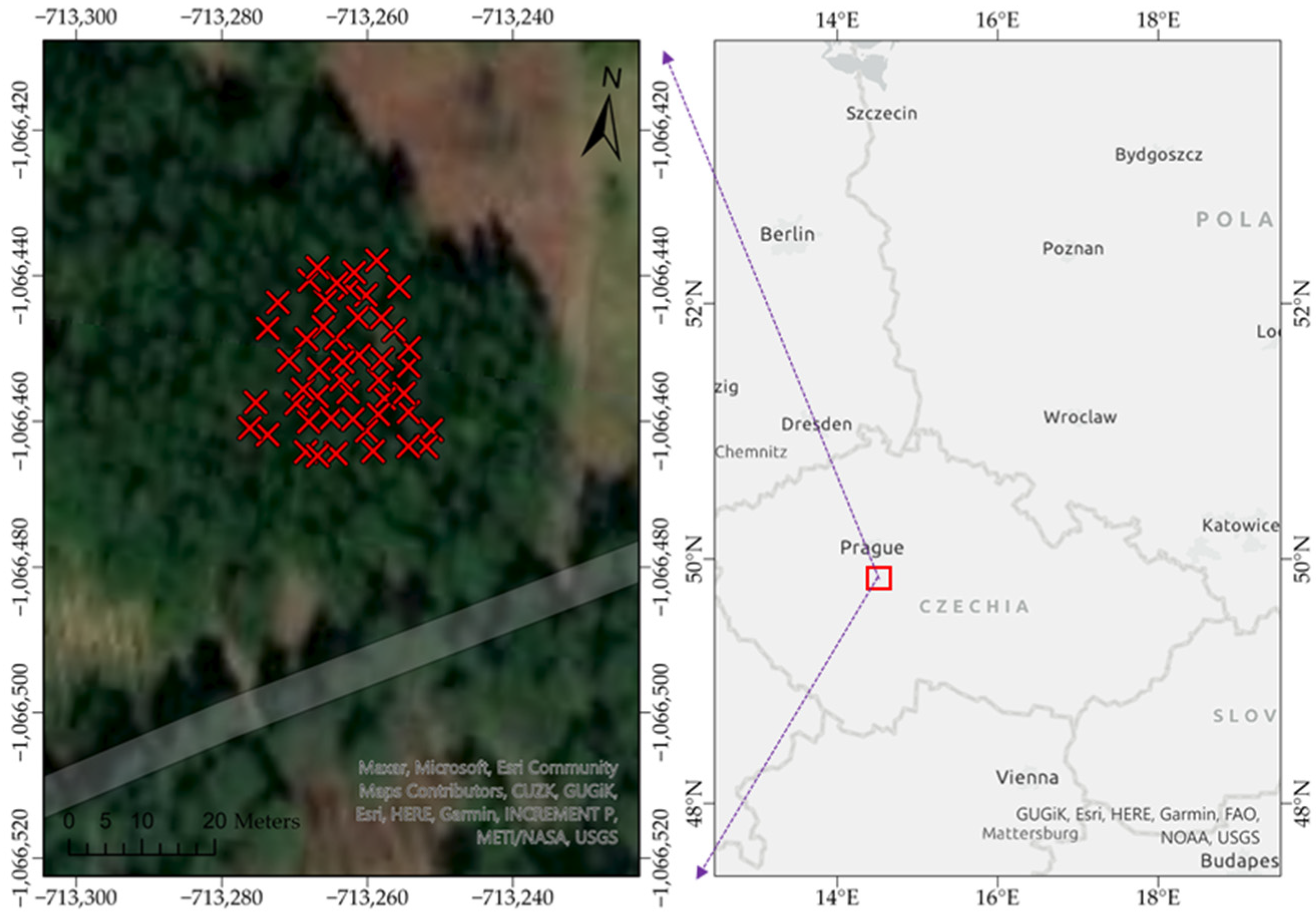
2.1. Characterization of the Test Site
2.2. Reference Data Acquisition
2.3. TLS Measurements
2.4. Point Cloud Normalization
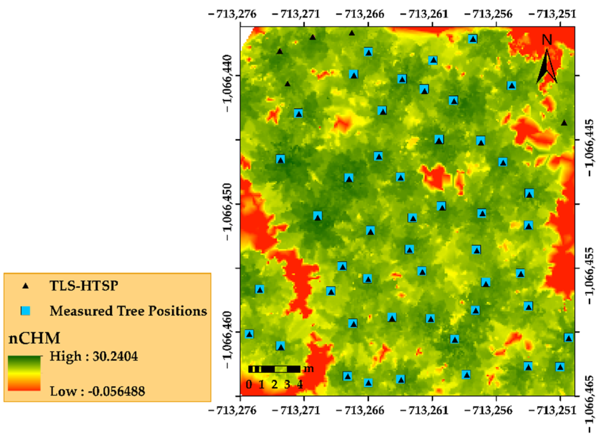
2.4.1. Total Stem Height Estimation from HTSP and Tree Locations
2.4.2. Total Stem Height Estimation Using the RANSAC Method
2.5. Diameter Estimation
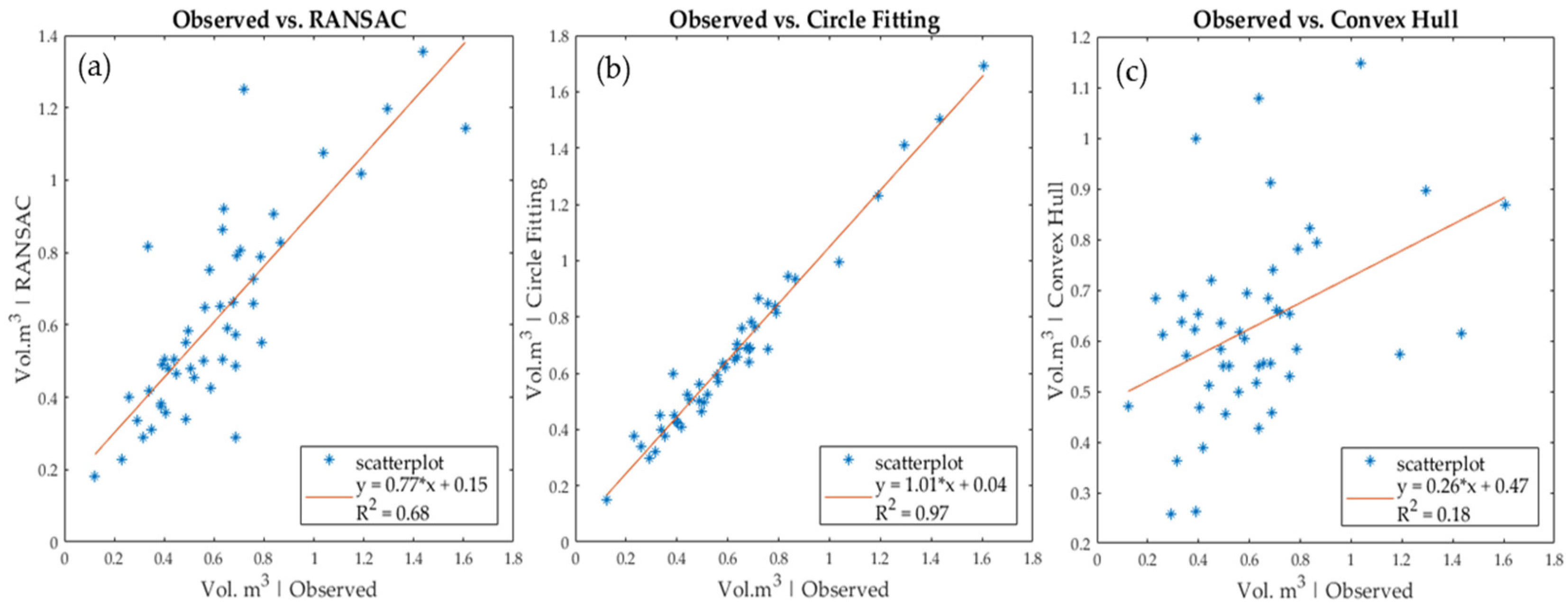
2.5.1. Geometric Approach by RANSAC
2.5.2. Algebraic Approach by Circle Fitting
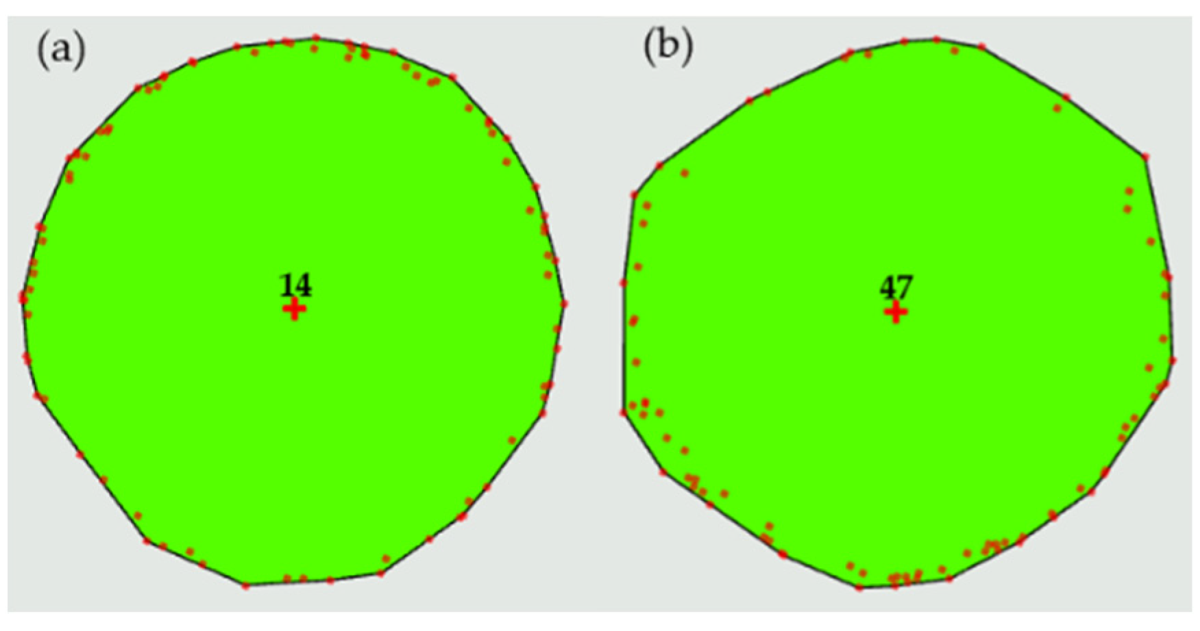
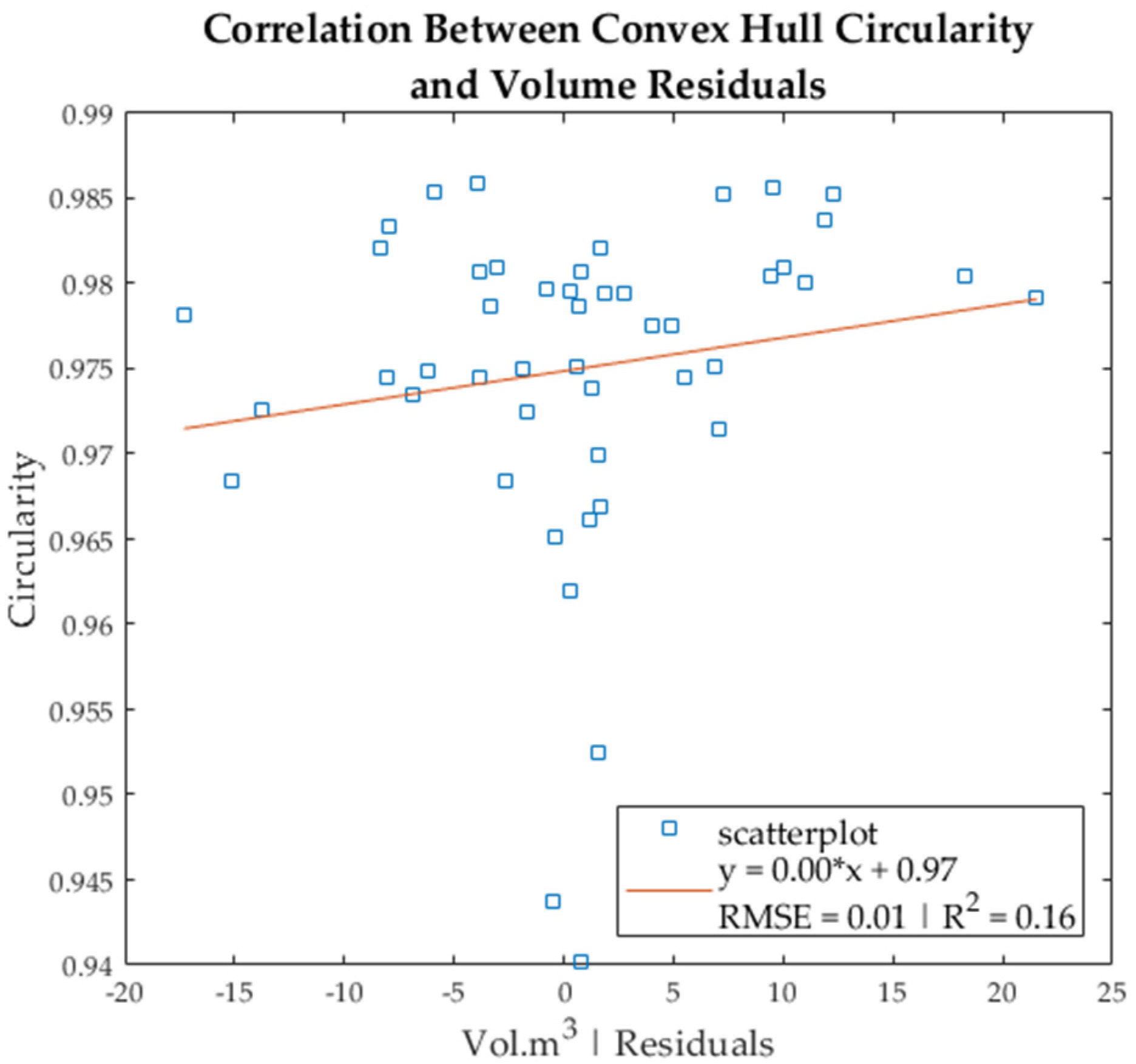
2.5.3. Geometric Approach by Convex Hull
2.6. Derivation of Total Stem Volume
2.7. Accuracy Assessment
3. Results and Discussion
4. Conclusions
Author Contributions
Funding
Institutional Review Board Statement
Informed Consent Statement
Data Availability Statement
Acknowledgments
Conflicts of Interest
References
- Kankare, V.; Vauhkonen, J.; Tanhuanpää, T.; Holopainen, M.; Vastaranta, M.; Joensuu, M.; Krooks, A.; Hyyppä, J.; Hyyppä, H.; Alho, P.; et al. Accuracy in estimation of timber assortments and stem distribution—A comparison of airborne and terrestrial laser scanning techniques. ISPRS J. Photogramm. Remote Sens. 2014, 97, 89–97. [Google Scholar] [CrossRef]
- Pretzsch, H.; Bielak, K.; Block, J.; Bruchwald, A.; Dieler, J.; Ehrhart, H.P.; Kohnle, U.; Nagel, J.; Spellmann, H.; Zasada, M.; et al. Productivity of mixed versus pure stands of oak (Quercus pretraea (Matt.) Liebl. and Quercus robur L.) and European beech (Fagus sylvatica L.) along an ecological gradient. Eur. J. For. Res. 2013, 132, 263–280. [Google Scholar] [CrossRef]
- Wang, Y.; Lehtomäki, M.; Liang, X.; Pyörälä, J.; Kukko, A.; Jaakkola, A.; Liu, J.; Feng, Z.; Chen, R.; Hyyppä, J. Is field-measured tree height as reliable as believed—A comparison study of tree height estimates from field measurement, airborne laser scanning and terrestrial laser scanning in a boreal forest. ISPRS J. Photogramm. Remote Sens. 2019, 147, 132–145. [Google Scholar] [CrossRef]
- Wang, Y.; Pyörälä, J.; Liang, X.; Lehtomäki, M.; Kukko, A.; Yu, X.; Kaartinen, H.; Hyyppä, J. In situ biomass estimation at tree and plot levels: What did data record and what did algorithms derive from terrestrial and aerial point clouds in boreal forest. Remote Sens. Environ. 2019, 232, 111309. [Google Scholar] [CrossRef]
- Forsman, M.; Börlin, N.; Holmgren, J. Estimation of tree stem attributes using terrestrial photogrammetry with a camera rig. Forests 2016, 7, 61. [Google Scholar] [CrossRef]
- Stereńczak, K.; Mielcarek, M.; Wertz, B.; Bronisz, K.; Zajączkowski, G.; Jagodziński, A.M.; Ochał, W.; Skorupski, M. Factors influencing the accuracy of ground-based tree height measurements for major European tree species. J. Environ. Manag. 2019, 231, 1284–1292. [Google Scholar] [CrossRef]
- Panagiotidis, D.; Abdollahnejad, A.; Slavík, M. Assessment of Stem Volume on Plots Using Terrestrial Laser Scanner: A Precision Forestry Application. Sensors 2021, 21, 301. [Google Scholar] [CrossRef]
- Vaunkonen, J.; Packalen, T. Uncertainties related to climate change and forest management with implications on climate regulation in Finland. Ecosyst. Serv. 2018, 33, 213–224. [Google Scholar] [CrossRef]
- Schneider, R.; Franceschini, T.; Fortin, M.; Saucier, J.P. Climate-induced changes in the stem form of 5 North American tree species. For. Ecol. Manag. 2018, 427, 446–455. [Google Scholar] [CrossRef]
- Panagiotidis, D.; Surový, P.; Kuželka, K. Accuracy of Structure from Motion models in comparison with terrestrial laser scanner for the analysis of DBH and height influence on error behaviour. J. For. Sci. 2016, 62, 357–365. [Google Scholar] [CrossRef]
- Panagiotidis, D.; Abdollahnejad, A.; Surový, P.; Chiteculo, V. Determining tree height and crown diameter from high-resolution UAV imagery. Int. J. Remote Sens. 2017, 38, 2392–2410. [Google Scholar] [CrossRef]
- Yrttimaa, T.; Luoma, V.; Saarinen, N.; Kankare, V.; Junttila, S.; Holopainen, M.; Hyyppä, J.; Vastaranta, M. Structural Changes in Boreal Forests Can Be Quantified Using Terrestrial Laser Scanning. Remote Sens. 2020, 12, 2672. [Google Scholar] [CrossRef]
- Abdollahnejad, A.; Panagiotidis, D.; Surový, P. Estimation and Extrapolation of Tree Parameters Using Spectral Correlation between UAV and Pléiades Data. Forests 2018, 9, 85. [Google Scholar] [CrossRef]
- Lizuka, K.; Hayakawa, Y.S.; Ogura, T.; Nakata, Y.; Kosugi, Y.; Yonehara, T. Integration of Multi-Sensor Data to Estimate Plot-Level Stem Volume Using Machine Learning Algorithms–Case Study of Evergreen Conifer Planted Forests in Japan. Remote Sens. 2020, 12, 1649. [Google Scholar]
- Pratt, V. Direct least-squares fitting of algebraic surfaces. Comput. Graph. 1987, 21, 145–152. [Google Scholar] [CrossRef]
- Kasa, I. A circle fitting procedure and its error analysis. IEEE Trans. Instrum. Meas 1976, IM–25, 8–14. [Google Scholar] [CrossRef]
- Taubin, G. Estimation of planar curves, surfaces, and non-planar space curves defined by implicit equations with applications to edge and range image segmentation. IEEE Trans. Pattern Anal. Mach. Intell. 1991, 13, 1115–1138. [Google Scholar] [CrossRef]
- Chernov, N. Circular and Linear Regression: Fitting Circles and Lines by Least Squares; Taylor & Francis: Boca Raton, FL, USA, 2011; ISBN 9781439835906. [Google Scholar]
- Fitzgibbon, A.; Pilu, M.; Fisher, R.B. Direct least square fitting of ellipses. IEEE Trans. Pattern Anal. Mach. Intell. 1999, 21, 476–480. [Google Scholar] [CrossRef]
- Fischler, M.A.; Bolles, R.C. Random sample consensus—A paradigm for model-fitting with applications to image-analysis and automated cartography. Commun. ACM 1981, 24, 381–395. [Google Scholar] [CrossRef]
- Schnabel, R.; Wahl, R.; Klein, R. Efficient RANSAC for Point-Cloud Shape Detection. Comput. Graph. Forum 2007, 26, 214–226. [Google Scholar] [CrossRef]
- Olofsson, K.; Holmgren, J.; Olsson, H. Tree Stem and Height Measurements using Terrestrial Laser Scanning and the RANSAC Algorithm. Remote Sens. 2014, 6, 4323–4344. [Google Scholar] [CrossRef]
- Panagiotidis, D.; Abdollahnejad, A.; Surový, P.; Kuželka, K. Detection of Fallen Logs from High-Resolution UAV Images. N. Z. J. For. 2019, 49. [Google Scholar] [CrossRef]
- Fan, G.; Nan, L.; Chen, F.; Dong, Y.; Wang, Z.; Li, H.; Chen, D. A New Quantitative Approach to Tree Attributes Estimation Based on LiDAR Point Clouds. Remote Sens. 2020, 12, 1779. [Google Scholar] [CrossRef]
- Mikita, T.; Janata, P.; Surový, P. Forest Stand Inventory Based on Combined Aerial and Terrestrial Close-Range Photogrammetry. Forests 2016, 7, 165. [Google Scholar] [CrossRef]
- Astrup, R.; Ducey, M.J.; Granhus, A.; Ritter, T.; Von Lüpke, N. Approaches for estimating stand-level volume using terrestrial laser scanning in a single-scan mode. Can. J. For. Res. 2014, 44, 666–676. [Google Scholar] [CrossRef]
- Mayamanikandan, T.; Reddy, R.S.; Jha, C. Non-Destructive Tree Volume Estimation using Terrestrial Lidar Data in Teak Dominated Central Indian Forests. In Proceedings of the 2019 IEEE Recent Advances in Geoscience and Remote Sensing: Technologies, Standards and Applications (TENGARSS), Kochi, India, 17–20 October 2019; pp. 100–103. [Google Scholar]
- Haglöf Sweden Laser Geo. Available online: https://haglofsweden.com/project/laser-geo-2 (accessed on 22 October 2003).
- Haglöf Sweden DP II Computer Caliper. Available online: https://haglofsweden.com/project/dp-ii-computer-caliper (accessed on 22 October 2003).
- Trimble Realworks 10.2 User Guide. 2017. Available online: https://www.trimble.com/3d-laser-scanning/realworks.aspx (accessed on 12 October 2019).
- Zhang, W.; Qi, J.; Wan, P.; Wang, H.; Xie, D.; Wang, X.; Yan, G. An Easy-to-Use Airborne LiDAR Data Filtering Method Based on Cloth Simulation. Remote Sens. 2016, 8, 501. [Google Scholar] [CrossRef]
- Girardeau-Montaut, D. CloudCompare. 2017. Available online: http://www.danielgm.org (accessed on 19 December 2016).
- ESRI ArcGIS Pro 2.4.2. Available online: https://www.esri.com/en-us/arcgis/products/arcgis-pro/resources (accessed on 21 May 2020).
- Corral-Rivas, J.J.; Barrio-Anta, M.; Aguirre-Calderón, O.A.; Diéguez-Aranda, U. Use of stump diameter to estimate diameter at breast height and tree volume for major pine species in El Salto, Durango (Mexico). Forestry 2007, 80, 29–40. [Google Scholar] [CrossRef]
- St-Onge, B.; Achaichia, N. Measuring forest canopy height using a combination of LIDAR and aerial photography data. Int. Arch. Photogramm. Remote Sens. Spat. Inf. Sci. 2001, 34, 22–24. [Google Scholar]
- About ArcGIS. Mapping & Analytics Software and Services. Available online: https://www.esri.com/en-us/arcgis/aboutarcgis/overview (accessed on 22 February 2021).
- Rousseeuw, P.J.; Kaufman, L. Finding groups in data. Ser. Probab. Math. Stat. 2003, 34, 111–112. [Google Scholar]
- Bucher, I. CircleFit. 2004. Available online: https://se.mathworks.com/matlabcentral/fileexchang/5557-circle-fit/content/circfit.m (accessed on 15 December 2016).
- Petráš, R.; Pajtík, J. Sústava česko-slovenských objemových tabuliek drevín. Lesn. Čas. 1991, 37, 49–56. [Google Scholar]
- Kořen, M.; Mokroš, M.; Bucha, T. Accuracy of tree diameter estimation from terrestrial laser scanning by circle-fitting methods. Int. J. Appl. Earth Obs. Geoinf. 2017, 63, 122–128. [Google Scholar] [CrossRef]
- Saarinen, N.; Kankare, V.; Vastaranta, M.; Luoma, V.; Pyorala, J.; Tanhuanpaa, T.; Liang, X.L.; Kaartinen, H.; Kukko, A.; Jaakkola, A.; et al. Feasibility of Terrestrial laser scanning for collecting stem volume information from single trees. ISPRS J. Photogramm. Remote Sens. 2017, 123, 140–158. [Google Scholar] [CrossRef]
- Pitkänen, T.P.; Raumonen, P.; Liang, X.; Lehtomäki, M.; Kangas, A. Improving TLS-based stem volume estimates by field measurements. Comput. Electron. Agric. 2021, 80, 105882. [Google Scholar] [CrossRef]
- Fassnacht, F.E.; Hartig, F.; Latifi, H.; Berger, C.; Hernández, J.; Corvalán, P.; Koch, B. Importance of sample size, data type and prediction method for remote sensing-based estimations of aboveground forest biomass. Remote Sens. Environ. 2014, 154, 102–114. [Google Scholar] [CrossRef]
- Shin, J.; Temesgen, H.; Strunk, J.L.; Hilker, T. Comparing Modeling Methods for Predicting Forest Attributes Using LiDAR Metrics and Ground Measurements. Can. J. Remote Sens. 2016, 42, 739–765. [Google Scholar] [CrossRef]


| Range Measurement | |
|---|---|
| Maximum Distance Range | 120 m on most surfaces |
| Range Systematic Error | <2 mm |
| Laser Wavelength | 1.5 µm, invisible |
| Laser Beam Diameter | 6–10–34 mm @ 10–30–100 m |
| Scanning Field-of-View | 360° × 317° |
| Scanning Speed | 1 million pts/s |
| Angular Accuracy | 80 µrad |
| Norway Spruce | A | B | C | E | F | G |
|---|---|---|---|---|---|---|
| Coefficients | 4.01 × 10⁻⁵ | 1.821816 | 1.132062 | 9.29 × 10⁻³ | −1.02037 | 0.896101 |
| N * | 48 |
| Chi-Square | 12.925 |
| Df * | 3 |
| Asymptotic Significance | 0.004801637 |
| Observed | Circle Fitting * | RANSAC | Convex Hull * | |
|---|---|---|---|---|
| Observed | - | 0.00 | 0.94 | 0.57 |
| Circle Fitting * | 0.00 | - | 0.06 | 0.63 |
| RANSAC | 0.94 | 0.06 | - | 0.70 |
| Convex Hull * | 0.57 | 0.63 | 0.70 | - |
| Method | Negative Rank (Observed > Estimated) | Positive Rank (Observed < Estimated) | Ties |
|---|---|---|---|
| RANSAC | 25 | 23 | 0 |
| Circle Fitting and HTSP | 6 | 42 | 0 |
| Convex Hull and HTSP | 23 | 25 | 0 |
| Observed Volume | Estimated Volume | |||
|---|---|---|---|---|
| RANSAC | Circle Fitting * | Convex Hull * | ||
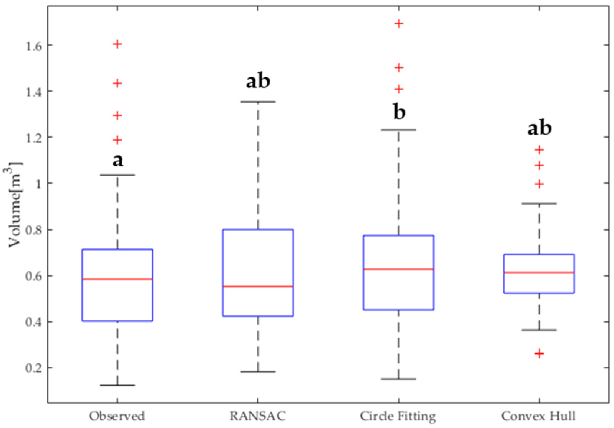
| Mean | 0.619 | 0.623 | 0.665 | 0.628 |
| Min | 0.123 | 0.182 | 0.151 | 0.258 |
| Q1 | 0.403 | 0.424 | 0.451 | 0.527 |
| Median | 0.584 | 0.551 | 0.627 | 0.613 |
| Q3 | 0.710 | 0.796 | 0.769 | 0.690 |
| Max | 1.606 | 1.354 | 1.694 | 1.147 |
| Bias | 0.000 | 0.004 | 0.046 | 0.009 |
| Bias% | 0.000 | 0.672 | 6.976 | 1.456 |
Publisher’s Note: MDPI stays neutral with regard to jurisdictional claims in published maps and institutional affiliations. |
© 2021 by the authors. Licensee MDPI, Basel, Switzerland. This article is an open access article distributed under the terms and conditions of the Creative Commons Attribution (CC BY) license (https://creativecommons.org/licenses/by/4.0/).
Share and Cite
Panagiotidis, D.; Abdollahnejad, A. Accuracy Assessment of Total Stem Volume Using Close-Range Sensing: Advances in Precision Forestry. Forests 2021, 12, 717. https://doi.org/10.3390/f12060717
Panagiotidis D, Abdollahnejad A. Accuracy Assessment of Total Stem Volume Using Close-Range Sensing: Advances in Precision Forestry. Forests. 2021; 12(6):717. https://doi.org/10.3390/f12060717
Chicago/Turabian StylePanagiotidis, Dimitrios, and Azadeh Abdollahnejad. 2021. "Accuracy Assessment of Total Stem Volume Using Close-Range Sensing: Advances in Precision Forestry" Forests 12, no. 6: 717. https://doi.org/10.3390/f12060717
APA StylePanagiotidis, D., & Abdollahnejad, A. (2021). Accuracy Assessment of Total Stem Volume Using Close-Range Sensing: Advances in Precision Forestry. Forests, 12(6), 717. https://doi.org/10.3390/f12060717