Article

Change of Potential Distribution Area of a Forest Tree Acer davidii in East Asia under the Context of Climate Oscillations

1
Shaanxi Key Laboratory for Animal Conservation, Key Laboratory of Resource Biology and Biotechnology in Western China (Ministry of Education), College of Life Sciences, Northwest University, Xi’an 710069, China
2
Early Life Institute, State Key Laboratory of Continental Dynamics, Department of Geology, Northwest University, Xi’an 710069, China
*
Author to whom correspondence should be addressed.
Forests 2021, 12(6), 689; https://doi.org/10.3390/f12060689
Submission received: 13 April 2021 / Revised: 22 May 2021 / Accepted: 24 May 2021 / Published: 27 May 2021

Abstract

:
The climate oscillations of the quaternary periods have profoundly affected the geographic distributions of current species. Acer davidii is a deciduous forest tree species mainly distributed in East Asia and China, playing a dominant role in the local forest ecosystem. In order to study the potential changes of geographic distributions of A. davidii in climate fluctuations, we collected the relate geographical distribution data and six climatic variables, using maximum entropy modelling to determine the species distribution. The results showed that the Areas Under Curve (AUC) values of the working characteristic curves of the subjects in the five historical periods were all greater than 0.93, suggesting that the results of maximum entropy modelling were accurate. The simulation of species distribution showed that the suitable area of A. davidii was mainly concentrated in central and northern China in contemporary times. From the Last Interglacial Age (LIG) to the Last Glacial Maximum (LGM), and then to the future (2050, 2070), the distribution area of this species experienced a decrease (LGM~Current; the high adaptability areas of central China became moderate) then an increase (Current~2050, the adaptation areas expanded to South Asia, Southeast Asia, and Siberia), and finally decreased (2050~2070, the suitable areas of South Asia, Southeast Asia, and Siberia shrank returning to China at latitude 25 °N). Compared to the LGM, the area of contemporary suitable area increased. Interestingly, the area of suitable growth range under future climatic conditions (2050) increased by half than before, and the suitable distribution area moved from Midwest China to Northeast China. This study on the change of species distribution can provide a typical case for the model study on the response of plants to climate change in the north temperate and subtropical zones of East Asia. Meanwhile, it can also give a basis for planting planning, species protection, and management.

1. Introduction

The relationship between the vegetation dynamic change and climate plays an important role in the field of global change. The prediction of the geographic distributions changes under the paleoclimate condition can provide an effective method for predicting the distribution area under future climate change [1]. Continuing global warming has a significant impact on global natural ecosystems. Thomas et al. [2], based on scenarios of moderate warming in 2050, have found that 15–37% of species in the sample areas (covering 20% of the Earth’s surface) will be at risk of extinction. Generally, climate change affects the geographical distribution of species, population growth, decline, and stability to a certain extent [3], and it has also been widely proved to have a great impact on community composition and structure [4,5], vegetation pattern, and ecosystem function [6]. Therefore, we predicted the species distribution dynamic of Acer davidii to understand the future distribution of these plants under climate change, which will be useful for planning adaptation to climate change in forestry and nature protection.
Species Distribution Modelling (SDM) is an important approach used to simulate the potential geographical distribution and ecological needs of species. Based on the contemporary environmental conditions of a species, this method can infer the potential suitable distribution areas in different geographical periods, and it was widely used in disciplines such as species protection and management [7,8]. The concept of realized niche shows the real distribution area of species in geographical space affected by biotic or abiotic factors [9]. In this study, we used “area of potential distribution” and “suitable area” to represent realized niches in different periods. As the absence records used by each model were different, the simulated realized niche was also different [10]. Currently, the two simulation methods, MaxEnt and GARP, are commonly used to predict the distributions of species on different scales [11,12]. Both models use artificial intelligence to assess potential geographical distribution. Of these, GARP uses specific rules to determine whether species exist in a given area and generates a model [13], while MaxEnt has recently been reclassified as a version of the generalized linear model. It generates the model based on the maximum entropy principle by finding the distribution closest to the uniform distribution in the whole study area of each environmental variable [14]. To study the distribution area changes of Tsoongiodendron odorum, Hu et al. [15] used MaxEnt to obtain the historical changes of the geographical distribution pattern of tourist trees, which provided data for conservation policy formulation in the future. Garza et al. [16] used MaxEnt to analyze the potential distribution area of the endemic plant Manihot walkerae in southeastern North America, which provided data support for future protection work. When the geographical location information of a species cannot be fully collected, GARP may perform better in predicting distribution [17]. On the other hand, MaxEnt has a high accuracy even when the species distribution data is very limited [12,18].
Recently, prediction research on species distribution area under climate change scenario has been conducted using species distribution data, environmental data, and prediction model methods, etc. Among them, multi-species distribution models and ensemble prediction based on multi-climate scenarios are becoming the main means and measures for species suitable habitat prediction under climate change [19,20]. However, most of the current studies focused on a certain period in the future, which could not reflect the overall trend of the change of species’ suitable habitats under the climate change scenario [21,22], and most of the previous studies only considered the change of suitable habitat areas, but not the changes of suitable degree, structure, and function of suitable habitats [23,24]. In addition, these studies did not take into account the effects of climate change on the suitable habitats by changing the distribution of vegetation types, soil environment, or other indirect ways [21,22].
Acer davidii Franchet, belonging to Aceraceae, is a deciduous forest tree species mainly distributed in East Asia, mainly in China. It often grows in sparse forests at an altitude of 500–1500 m [25]. It grows rapidly with a neat crown, so it can be used as a tree species for greening and afforestation. The long bark fiber containing tannins can be used as industrial raw material [25]. Shading can improve the adaptation of A. davidii seedlings to the environment [26]. In the effect of radiation on plants, Li et al. [27] found that UV-B radiation had some inhibitory effects on the photosynthesis of A. davidii seedlings.
At present, there are few studies on the simulation of species distribution of Acer species. Previous studies mainly focused on the external environmental influence on its physiological activities. For instance, Hanba et al. [28] found that there were great differences in light demand of leaves between different Acer species. Coudun et al. [29] found that the nutrient composition of the soil had a great influence on the distribution of Acer campestre; Kim et al. [30] extracted vitexin from Acer palmatum, which has isolation and antioxidant effects; Tsuda et al. [31] found out the reason why Acer saccharinum, as a riparian species, can grow well in dry soil after transplantation; Royer et al. [32] showed the high correlation between annual mean temperature and the leaf size of Acer rubrum, which can be used to the reconstruct paleoclimate model. In the context of climate change, the study on potential distribution is becoming especially important for species conservation and resource utilization. Taking China as an example, Acer species in China are widely spread. However, the environmental factors in the distribution area are quite different, and the distribution information of Acer species in some areas is still not clear, which are the reasons for the lack of simulation research on the Acer distribution area.
In this study, the Chinese endemic species A. davidii was used to study the change of its suitable area under the scenario of climate change. The purpose of this study is to understand the impact of climate change on the distribution of A. davidii since the Last Glacial Maximum to determine the important environmental factors that affect its distribution and to predict the change of its suitable areas, so as to provide theoretical reference and scientific basis for the protection and utilization of A. davidii. Meanwhile, this study can provide a typical case for the model study of the response of plants to climate change in the north temperate zone and subtropics of East Asia, and it can also provide an example for the response analyses of other taxa in the region to climate and environmental change.

2. Materials and Methods

2.1. Data Sources

Geographical information of A. davidii: We obtained a total of 287 occurrences of A. davidii by field works or from the China Digital Plant Museum (http://www.cvh.org.cn) and GBIF Database (http://www.gbif.org/) at January 2021. After examination, uncertain and repeated sample points were removed. In total, 262 distribution points, which can be used to perform the MaxEnt model program, were retained, and ArcGIS10.7 was used to draw the geographical distribution map (Figure 1) of A. davidii. The elevation data were downloaded from the National basic Geographic Information Center (http://www.ngcc.cn/ngcc/) at January 2021.
Environmental variable information: The climate variable data were obtained from the world climate database (WorldClim, http:///www.wordclim.org/) at January 2021. The climatic data for each period include 19 bioclimatic variables (bio01–bio19), for which the spatial resolution was 2.5 min in this study.

2.2. Environmental Factors and Pretreatment

We deleted the sample points that could not be acerated and finally obtained a total of 262 sample points. In order to avoid the overfitting phenomenon caused by the high correlation of environmental variables, we evaluated the contribution rate of each variable through the knife-cutting method of the MaxEnt model and obtained the pre-selected environmental variables combined with the results of the response curve. The environmental variable information of the 262 A. davidii samples was extracted using ArcGIS10.7 Esri, and then the Spearman correlations between environmental variables were calculated using SPSS Statiatics software (Table S1). If the correlation coefficient of the two variables was more than |0.85|, only one of the two variables with high contribution rate was selected because multicollinearity may violate statistical assumptions and alter model predictions [33]. The environmental factors obtained by the above method are shown in Table 1.

2.3. Models and Methods

The distribution with the maximum entropy is closest to the real state. The maximum entropy principle for data analysis was selected as the MaxEnt model to calculate the probability distribution with maximum entropy that satisfies the distribution constraints, so that the probability distribution of random events could be inferred from incomplete information. MaxEnt combines statistical models and machine learning to simulate speciation, using only a small amount of given data. Its simulation accuracy is higher than that of other models, and the prediction effect is better. When using a computer to simulate the distribution of entropy, the MaxEnt model takes the pixels of known species distribution points as samples, obtains the constraint conditions according to its environmental variables, such as climate, altitude, and soil type, and explores the possible distribution of maximum entropy under these constraints, so as to predict the distribution of species in the study area [34]. The maximum entropy algorithm is a constrained optimization algorithm, i.e., when the output is known. For a given training data set and characteristic function f i ( x , y ) ,   i = 1 , 2 , , n , MaxEnt solves the equation as follows:
max p c H ( P ) x , y P ˜ ( x ) P ( y | x ) log P ( y | x )
s . t .   E p ( f i ) = E p ˜ ( f i ) ,   i = 1 , 2 , , n
y P ( y | x ) = 1
where H ( P ) is conditional entropy, P ( y | x ) is conditional probability distribution hypothesis, P ˜ ( x ) is empirical distribution, and E p ( f i ) represents the expectation of the characteristic function, with respect to the empirical distribution.
Based on probability theory and machine learning, this model was constructed using species distribution points and environmental variables. In order to improve the accuracy of prediction, this study randomly selected 75% of the total data as the training set to build the model, and the remaining 25% was used to test the model. Additionally, the MaxEnt model was randomly selected as the training set. The potential distribution areas of A. davidii in the Last Glacial Maximum (LGM), the Last Interglacial (LIG), the present and the future (2050, 2070) were simulated. By using the natural segment method in ArcGIS, the distribution area of each period simulated in MaxEnt was divided into four grades: non-adaptive area, low-adaptive area, moderate-adaptive area, and high-adaptive area.

2.4. Model Result Evaluation

The accuracy of the MaxEnt model was tested by the subject working characteristic curve Receiver Operator Characteristic curve (ROC), which was represented as by the area under the curve (AUC). The value range was between 0 and 1, and the larger the AUC value is, the more accurate the model prediction is. Specifically, when the AUC value is between 0.5 and 0.6, the simulation of the model “fails”; the AUC value of 0.6–0.7 indicates that the simulation effect of the model is “poor”; the AUC value of 0.7–0.8 indicates that the simulation effect of the model is “general”; the AUC value of 0.8–0.9 indicates that the simulation effect of the model is “good”, and the AUC value greater than 0.9 indicates that the simulation effect of the model is “excellent” [35], which can accurately reflect the potential distribution of species. The model uses cloglog as the output format. MIROC is a model designed by the Japanese to simulate climate change in East Asia [36], and CCSM is a model designed by Americans to simulate global climate change, so the results simulated by MIROC should be more accurate than those simulated by CCSM in this study. In addition, some studies have found that the high concentration of RCP8.5 may overestimate the future supply of fossil fuels [37]. According to the report on future coal use, 90% of fossil fuels will be exhausted by 2070 [38]. Therefore, we chose RCP6.0, which assumes that greenhouse gases will peak in 2080 [39]. We also simulated the two climate scenarios of RCP2.6 and RCP4.5 to analyze the distribution area of A. davidi. We used response curves to analyze and discuss the influences of different environmental variables on the potential distribution area and the relationship between distribution and environmental factors.

3. Results

3.1. Evaluation of the Accuracy of the Model

Using 262 contemporary distribution records and 6 climate variables, the maximum entropy model was used to simulate the potential geographical distribution of A. davidii. As shown in Figure 2, in the Last Glacial Maximum (LGM), Last Interglacial (LIG), current and future (2050 and 2070) simulations, the values of AUC were all greater than 0.93, indicating that the prediction results were accurate. We chose MIROC to simulate our data.

3.2. Importance of Variables and Climate Preference

Table 2 shows the contribution rate and importance of environmental variables to the distribution of A. davidii in different periods. In the Last Glacial Maximum (MIROC, CCSM), last interglacial, present and future (2050, 2070) simulations, the top three environmental factors were the mean temperature of the coldest quarter, precipitation of the warmest quarter, and annual precipitation. For every simulated period, the most important environmental factor was the mean temperature of the coldest quarter.
As shown in Figure 3, in the regularization training gain, the proportion of environmental factors in the Last Glacial Maximum, the Last Interglacial, contemporary and 2070 simulations were the same from high to low as the mean temperature of the coldest quarter, precipitation of the warmest quarter, temperature seasonality, precipitation of the wettest quarter, annual precipitation, and precipitation of the wettest month. The proportion of environmental factors from high to low in 2050 was a mean temperature of the coldest quarter, temperature seasonality, precipitation of the wettest month, precipitation of the wettest quarter, annual precipitation, and precipitation of the warmest quarter.
As shown in Figure 4, in the test training gain, the proportion of MIROC in the Last Glacial Maximum was the same as that of contemporary environmental factors, and the contribution rate of this period was the mean temperature of the coldest quarter, precipitation of the warmest quarter, temperature seasonality, precipitation of the wettest quarter, precipitation of the wettest month, and annual precipitation. The proportion of environmental factors in the last glacial maximum (CCSM) and sub-interglacial (LIG) was the same as that in 2070, and the order from high to low was the mean temperature of the coldest quarter, precipitation of the warmest quarter, temperature seasonality, precipitation of the wettest quarter, annual precipitation, and precipitation of the wettest month. The proportion of environmental factors from high to low in 2050 was the mean temperature of the coldest quarter, temperature seasonality, precipitation of the wettest month, precipitation of the wettest quarter, annual precipitation, and precipitation of the warmest quarter.
All results indicated that the main environmental variables affecting the potential distribution area of A. davidii were temperature (mean temperature of the coldest quarter, SD of temperature change) and precipitation (precipitation of the warmest quarter, precipitation of the wettest quarter).

3.3. Threshold Analysis of Dominant Environmental Variables

The analyses of those response curves (Figure 5) also indicated how the logistic prediction for A. davidii changed. It indicated that the threshold values of SD of temperature change was 2310 and 12,560, precipitation of the wettest quarter was 195 and 2000 mm, precipitation of the warmest quarter was 190 and 30,250 mm, and mean temperature of the coldest quarter was 110 and 210 °C. The highest points of the images represent their optimal threshold, which means that the temperature or humidity is most suitable for A. davidii to grow.

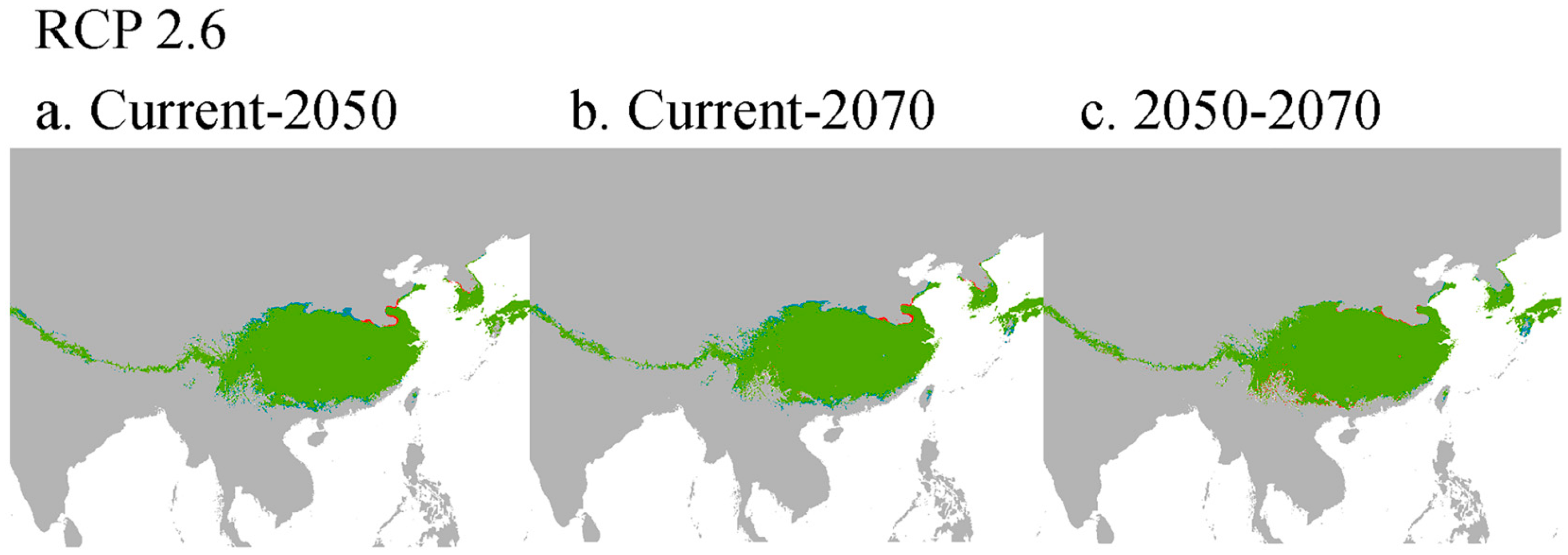
3.4. Changes of Potential Geographical Distribution of A. davidii in Asia under Different Climatic Scenarios

The distribution area of A. davidii changed in different periods. The main contemporary distribution areas of A. davidii are located in Yunnan, Guangxi, Guizhou, Chongqing, Sichuan, Gansu, Shanxi, Shaanxi, Ningxia, Hebei, Beijing, Tianjin, Shandong, Anhui, Jiangsu, Hubei, Henan, Shanghai, Fujian, Taiwan, and Guangdong. Because the AUC predicted by MIROC was greater than CCSM, compared with the Last Glacial Maximum (MIROC), the total area of contemporary distribution increased by 28.6059 km2 (0.68%). The area of the high adaptation area decreased by 23.1129 km2 (0.52%); the area of the medium adaptation area increased by 11.2708 km2 (0.22%); and the area of the low adaptation area increased by 5.7778 km2 (0.97%). Compared to the Last Interglacial Age (LIG), the total current distribution area increased by 92.5365 km2 (4.55%). The high-growth area increased by 41.1545 km2 (2.05%); the medium-adapted area increased by 58.4966 km2 (2.92%); and the low-adapted area decreased by 7.1146 km2 (0.43%). In 2050, new potential distribution areas appeared in Siberia, South Asia, and Southeast Asia, and the proportion of potential distribution areas in Korean Peninsula and Japan increased. The total area of potential distribution in 2050 accounted for 1058.2361 km2 (37.16%) of the total area. Compared to the present age, the total area of 2070 increased by 402.7378 km2 (19.97%). Other detailed information about distribution change is shown in Table 3 and Table 4.
According to Figure 6, during the last glacial maximum, the suitable areas were mainly concentrated in the vicinity of latitude 30 °N, and the high-adaptive areas were mainly distributed in Sichuan, Guizhou, and Zhejiang, China, and near the junction of Honshu and Kyushu in Japan (Figure 6a,b). With the arrival of the last interglacial age, the suitable area shrank and moved southward, mainly concentrated in the latitude of 25 °N, and the main high growth areas tended to transfer from Sichuan to Yunnan (Figure 6c). However, the suitable area expanded significantly in 2050, in which the high-adaptive area moved to northeastern China and a new high-adaptive area began to appear in Baikal Lake and southwestern India (Figure 6e). In 2070, the suitable area moved significantly to the south and the high-adaptive area was mainly located in the vicinity of latitude 20 °N. New high suitable areas emerged in Laos, Myanmar, Vietnam, and the island countries in the Pacific Ocean. The Korean Peninsula and Japan also became very suitable for the growth of A. davidii (Figure 6f).
Figure 7 shows more clearly the changes of the potential distribution area of A. davidii in the future (RCP 6.0). Although part of the current suitable area of A. davidii would be lost in 2050 due to climate change, the total distribution area would experience a large-scale expansion. Compared with the present age, the distribution area of A. davidii would gradually move southward in 2070, and most of the current distribution area would no longer be suitable for its growth. Although the area of potential distribution would be much smaller than that in 2050, it would still be larger than the current area.
Figure 8 and Figure 9 show the distribution areas of A. davidii in RCP 2.6 and RCP 4.5 scenarios, and the change trend in each period was the same as RCP 6. With the decrease of pollutant discharge, the expansion of the distribution area of A. davidii became smaller but more stable.

4. Discussion

Climate change will have different effects on plants in different geographic regions [40]. The adaptability of species to different environmental variables is the decisive factor of their distribution patterns [42]. Since the late Pleistocene, the global climate has fluctuated greatly, especially the last glacial-interglacial cycle, which has profoundly affected the distribution of most organisms at present [43,44]. In this study, the Jackknife test of the Maxent model was used to analyze the environmental factors that affect the distribution of A. davidii. The results suggest that the mean temperature of the coldest quarter, precipitation of the warmest quarter, temperature seasonality, and precipitation of the wettest quarter were the main factors affecting the potential geographical distribution of A. davidii, and the mean temperature of the coldest quarter made the greatest contribution to it. Since the seasonality of temperature usually increases with the increase of latitude [45], it may determine the upper limit of the distributed latitude of A. davidii. The change of temperature affects the distribution of seeds by affecting seed germination, water absorption, photosynthesis, transpiration, respiration, reproduction, and growth [17]. Precipitation affects the growth, morphology, phenological phase, and plant biomass accumulation of A. davidii, resulting in a decrease in plant height and seed yield, thus affecting its distribution [46,47]. Therefore, all these factors will affect the final ecological adaptation and distribution of A. davidii. Additionally, according to the results of three different climate scenarios, the higher the emission level of pollutants, the more unstable the distribution area of A. davidii, which indirectly reflects the intensity of climate change. Meanwhile, the results of RCP 2.6 and RCP 4.5 are very similar, which indicates that there is a critical value of the impact of pollutant emissions on environmental change [40,41].
Compared to the change of suitable area, each species’ research results were different. The distribution area of different species showed different trends under the influence of the same environmental factors. For example, Acer palmatum Thunb., which was distributed on the edge of subtropical forests in China, North Korea, and Japan or in sparse forests at low altitudes belongs to the same genus and growth in a similar habitat to A. davidii. Gao et al. [48] studied the spatial distribution of Acer palmatum and found that the suitable area of this species expanded at first and then shrank. However, Lin et al. [49] draew a different conclusion in the simulation of the distribution area of another Acer species, Acer ginnala Maxim., which was distributed on the jungle below, 800 m above sea level. This species was sensitive to temperature and precipitation, similar to A. davidii. The suitable area of Acer ginnala Maxim is predicted to gradually decrease in the future.
Additionally, plants affected by the same environmental variables are supposed have similar changes in the distribution area during climate change. Therefore, we can test the accuracy of the prediction by referring to plants with the same sensitive environmental variables as the A. davidii. With climate change, the increasing temperature has turned previously colder high latitudes into environments suitable for plant growth, thus accelerating the process of plant migration [50]. The simulation results of Jin et al. [51] on the future distribution area of Phyllostachys edulis, distributed in the temperate zone with annual precipitation between 1200 mm and 1800 mm, showed that the species tended to migrate to high latitudes. When Jiang et al. [52] studied the geographical distribution simulation of three endangered wild grape species Vitis L. in China, which are distributed in the Yangtze River basin and are sensitive to temperature and precipitation, the suitable areas of the threes species were found to expand northward in the future. The suitable areas of these two taxa are similar to those of A. davidii, and their simulation results are consistent with our research, which confirms the accuracy of our results. In our study, the high adaptive area of A. davidii moved from central China (Sichuan, Guizhou, and Chongqing) to northeast China and Siberia in 2050, which also supported the above point of view. As mankind takes more active action against climate warming, the southward shift of the suitable area of A. davidii in 2070 confirms the impact of climate change on species distribution.
Comparing the reconstructed distribution area under paleoclimate with that predicted under a future climate model can provide better methods and strategies for species protection and utilization [53]. Due to the wide distribution of A. davidii, most sampling sites lack more accurate coordinate information, which may lead to the inaccuracy of the prediction results. At the same time, topography, soil, biological invasion, human activities [54], and other factors were not considered in this study. In particular, with the increasingly frequent long-distance biological communication, it is very important to consider the impact of biological invasion on the species distribution area [55]. In future research, these factors should be further discussed to increase the screening range of environmental variables to improve the accuracy. In the actual living environment, species interaction, vegetation types, geomorphological features, and species diffusion ability will have a certain impact on the potential suitable area of predicted species [56]. Therefore, the prediction result in this study only shows the possible species distribution, but it cannot accurately reflect the actual distribution area of species, since the various environmental factors we described above may have an impact on the changes of the distribution area. Despite this, this study can still provide a typical case for the model study of the response of plants in East Asia to deal with climate change and can provide theoretical support for further introduction and cultivation of A. davidii, for which the afforestation and function as excellent industrial raw materials may be utilized better. New guidelines will need to be created as a strategy. For example, assisted migration may help A. davidii reach a new place when the origin site is no longer suitable to grow due to climate changes [57].

5. Conclusions

SDM has showed its ability for providing strategies under global climate change [57]. According to our study on A. davidii, the accuracy of prediction under MIROC is higher than that under CCSM. The main climatic factors affecting the distribution of A. davidii in different periods were temperature (mean temperature of the coldest quarter, min temperature of coldest month, temperature annual range) and water (precipitation of the warmest quarter). Compared with the Last Glacial Maximum (LGM) and the Last Interglacial Age (LIG), the contemporary distribution area increased. Compared with the present age, the distribution area increased by 52.76% in 2050 and 19.97% in 2070. Under the influence of climatic factors, the high fitness area showed an overall upward trend, but compared with 2050, the high fitness area in 2070 will decrease by 0.24%. The medium suitable area will be reduced by 29.24%, and the low suitable area will be reduced by 3.32%. In addition, due to the fact that influences of soil and other factors in the distribution area were not taken into account, the range of environmental conditions simulated in this study may be larger than the actual condition.

Supplementary Materials

The following are available online at https://www.mdpi.com/article/10.3390/f12060689/s1, Table S1: Linear correlation analysis among variables by Spearman coefficient.

Author Contributions

Conceptualization, Z.L. and Z.S.; methodology, Z.L.; software, Z.S.; validation Z.S., X.S., and X.H.; formal analysis, Q.Z., A.F., and Z.S.; investigation, Z.S.; resources, M.L.; data curation, J.L.; writing—original draft preparation, Z.S.; writing—review and editing, Z.L., Y.K., J.T., and Z.S.; visualization, Z.S.; supervision, Z.L.; project administration, Z.L.; funding acquisition, Z.L. and Y.K. All authors have read and agreed to the published version of the manuscript.

Funding

This work was financially supported by the National Natural Science Foundation of China (31872263 and 31970359), the Shaanxi Science and Technology Innovation Team (2019TD-012), and the Fourth National Survey of Traditional Chinese Medicine Resources (2018-43 and 2019-68).

Institutional Review Board Statement

Not applicable.

Informed Consent Statement

Not applicable.

Conflicts of Interest

The authors declare no conflict of interest.

References

  1. Cong, M.; Xu, Y.; Tang, L.; Yang, W.; Jian, M. Predicting the dynamic distribution of Sphagnum bogs in China under climate change since the last interglacial period. PLoS ONE 2020, 15. [Google Scholar] [CrossRef] [PubMed]
  2. Thomas, C.D.; Cameron, A.; Green, R.E.; Bakkenes, M.; Beaumont, L.J.; Collingham, Y.C.; Erasmus, B.F.N.; de Siqueira, M.F.; Grainger, A.; Hannah, L.; et al. Extinction risk from climate change. Nature 2004, 427, 145–148. [Google Scholar] [CrossRef] [PubMed]
  3. Fitzpatrick, M.C.; Gove, A.D.; Sanders, N.J.; Dunn, R.R. Climate change, plant migration, and range collapse in a global biodiversity hotspot: The Banksia (Proteaceae) of Western Australia. Glob. Chang. Biol. 2008, 14, 1337–1352. [Google Scholar] [CrossRef]
  4. Alberto, F.J.; Aitken, S.N.; Alia, R.; Gonzalez-Martinez, S.C.; Hanninen, H.; Kremer, A.; Lefevre, F.; Lenormand, T.; Yeaman, S.; Whetten, R.; et al. Potential for evolutionary responses to climate change evidence from tree populations. Glob. Chang. Biol. 2013, 19, 1645–1661. [Google Scholar] [CrossRef] [Green Version]
  5. Xu, H.-J.; Wang, X.-P.; Zhao, C.-Y.; Yang, X.-M. Diverse responses of vegetation growth to meteorological drought across climate zones and land biomes in northern China from 1981 to 2014. Agric. For. Meteorol. 2018, 262, 1–13. [Google Scholar] [CrossRef]
  6. Bellard, C.; Bertelsmeier, C.; Leadley, P.; Thuiller, W.; Courchamp, F. Impacts of climate change on the future of biodiversity. Ecol. Lett. 2012, 15, 365–377. [Google Scholar] [CrossRef] [PubMed] [Green Version]
  7. Peterson, A.T.; Papes, M.; Eaton, M. Transferability and model evaluation in ecological niche modeling: A comparison of GARP and Maxent. Ecography 2007, 30, 550–560. [Google Scholar] [CrossRef]
  8. Li, Y.; Tang, Z.; Yan, Y.; Wang, K.; Cai, L.; He, J.; Gu, S.; Yao, Y. Incorporating species distribution model into the red list assessment and conservation of macrofungi: A case study with Ophiocordyceps sinensis. Biodivers. Sci. 2020, 28, 99–106. [Google Scholar] [CrossRef] [Green Version]
  9. Hutchinson, G.E. Population studies—Animal ecology and demography—Concluding remarks. Cold Spring Harb. Symp. Quant. Biol. 1957, 22, 415–427. [Google Scholar] [CrossRef]
  10. Soberon, J. Grinnellian and Eltonian niches and geographic distributions of species. Ecol. Lett. 2007, 10, 1115–1123. [Google Scholar] [CrossRef]
  11. Guisan, A.; Zimmermann, N.E. Predictive habitat distribution models in ecology. Ecol. Model. 2000, 135, 147–186. [Google Scholar] [CrossRef]
  12. Elith, J.; Graham, C.H.; Anderson, R.P.; Dudik, M.; Ferrier, S.; Guisan, A.; Hijmans, R.J.; Huettmann, F.; Leathwick, J.R.; Lehmann, A.; et al. Novel methods improve prediction of species’ distributions from occurrence data. Ecography 2006, 29, 129–151. [Google Scholar] [CrossRef] [Green Version]
  13. David, R.B.; Stockwell, I.R.N. Induction of sets of rules from animal distribution data: A robust and informative method of data analysis. Math. Comput. Simul. 1992, 33, 385–390. [Google Scholar]
  14. Phillips, S.J.; Anderson, R.P.; Schapire, R.E. Maximum entropy modeling of species geographic distributions. Ecol. Model. 2006, 190, 231–259. [Google Scholar] [CrossRef] [Green Version]
  15. Hu, W.; Zhang, Z.-Y.; Chen, L.-D.; Peng, Y.-S.; Wang, X. Changes in potential geographical distribution of Tsoongiodendron odorum since the Last Glacial Maximum. Chin. J. Plant Ecol. 2020, 44, 44–55. [Google Scholar] [CrossRef]
  16. Garza, G.; Rivera, A.; Venegas Barrera, C.S.; Guadalupe Martinez-Avalos, J.; Dale, J.; Arroyo, T.P.F. Potential Effects of Climate Change on the Geographic Distribution of the Endangered Plant Species Manihot walkerae. Forests 2020, 11, 689. [Google Scholar] [CrossRef]
  17. Costa, G.C.; Nogueira, C.; Machado, R.B.; Colli, G.R. Sampling bias and the use of ecological niche modeling in conservation planning: A field evaluation in a biodiversity hotspot. Biodivers. Conserv. 2010, 19, 883–899. [Google Scholar] [CrossRef]
  18. Hernandez, P.A.; Graham, C.H.; Master, L.L.; Albert, D.L. The effect of sample size and species characteristics on performance of different species distribution modeling methods. Ecography 2006, 29, 773–785. [Google Scholar] [CrossRef]
  19. Leng, W.; He, H.S.; Bu, R.; Dai, L.; Hu, Y.; Wang, X. Predicting the distributions of suitable habitat for three larch species under climate warming in Northeastern China. For. Ecol. Manag. 2008, 254, 420–428. [Google Scholar] [CrossRef]
  20. Zhang, K.; Sun, L.; Tao, J. Impact of Climate Change on the Distribution of Euscaphis japonica (Staphyleaceae) Trees. Forests 2020, 11, 525. [Google Scholar] [CrossRef]
  21. Lin, L.; He, J.; Xie, L.; Cui, G. Prediction of the Suitable Area of the Chinese White Pines (Pinus subsect. Strobus) under Climate Changes and Implications for Their Conservation. Forests 2020, 11, 996. [Google Scholar] [CrossRef]
  22. Zhao, R.; Chu, X.; He, Q.; Tang, Y.; Song, M.; Zhu, Z. Modeling Current and Future Potential Geographical Distribution of Carpinus tientaiensis, a Critically Endangered Species from China. Forests 2020, 11, 774. [Google Scholar] [CrossRef]
  23. Velasquez-Tibata, J.; Salaman, P.; Graham, C.H. Effects of climate change on species distribution, community structure, and conservation of birds in protected areas in Colombia. Reg. Environ. Chang. 2013, 13, 235–248. [Google Scholar] [CrossRef]
  24. Valle, M.; Chust, G.; del Campo, A.; Wisz, M.S.; Olsen, S.M.; Garmendia, J.M.; Borja, A. Projecting future distribution of the seagrass Zostera noltii under global warming and sea level rise. Biol. Conserv. 2014, 170, 74–85. [Google Scholar] [CrossRef]
  25. Editorial Committee of Chinese Flora. Flora of China; Beijing Science Press: Beijing, China, 1993. [Google Scholar]
  26. Guo, X.; Luo, Y.J.; Xu, Z.W.; Li, M.Y.; Guo, W.H. Response strategies of Acer davidii to varying light regimes under different water conditions. Flora 2019, 257. [Google Scholar] [CrossRef]
  27. Zuo, W.; Liu, Q.; Lin, B.; He, H. Physiological responses of 2-year-old Acer davidii seedlings to short-term enhanced UV-B radiation. J. Appl. Ecol. 2005, 16, 1682–1686. [Google Scholar]
  28. Hanba, Y.T.; Kogami, H.; Terashima, I. The effect of growth irradiance on leaf anatomy and photosynthesis in Acer species differing in light demand. Plant Cell Environ. 2002, 25, 1021–1030. [Google Scholar] [CrossRef]
  29. Coudun, C.; Gegout, J.-C.; Piedallu, C.; Rameau, J.-C. Soil nutritional factors improve models of plant species distribution: An illustration with Acer campestre (L.) in France. J. Biogeogr. 2006, 33, 1750–1763. [Google Scholar] [CrossRef]
  30. Kim, J.H.; Lee, B.C.; Kim, J.H.; Sim, G.S.; Lee, D.H.; Lee, K.E.; Yun, Y.P.; Pyo, H.B. The isolation and antioxidative effects of vitexin from Acer palmatum. Arch. Pharm. Res. 2005, 28, 195–202. [Google Scholar] [CrossRef]
  31. Tsuda, M.; Tyree, M.T. Whole-plant hydraulic resistance and vulnerability segmentation in Acer saccharinum. Tree Physiol. 1997, 17, 351–357. [Google Scholar] [CrossRef] [Green Version]
  32. Royer, D.L.; McElwain, J.C.; Adams, J.M.; Wilf, P. Sensitivity of leaf size and shape to climate within Acer rubrum and Quercus Kelloggii. New Phytol. 2008, 179, 808–817. [Google Scholar] [CrossRef] [PubMed]
  33. Heikkinen, R.K.; Luoto, M.; Araujo, M.B.; Virkkala, R.; Thuiller, W.; Sykes, M.T. Methods and uncertainties in bioclimatic envelope modelling under climate change. Prog. Phys. Geogr. 2006, 30, 751–777. [Google Scholar] [CrossRef] [Green Version]
  34. Swets, J.A. Measuring the accuracy of diagnostic systems. Science 1988, 240, 1285–1293. [Google Scholar] [CrossRef] [Green Version]
  35. Rong, Z.; Zhao, C.; Liu, J.; Gao, Y.; Zang, F.; Guo, Z.; Mao, Y.; Wang, L. Modeling the Effect of Climate Change on the Potential Distribution of Qinghai Spruce (Picea crassifolia Kom.) in Qilian Mountains. Forests 2019, 10, 62. [Google Scholar] [CrossRef] [Green Version]
  36. Nozawa, T.; Ogura, T.; Yokohata, T.; Okada, N.; Shiogama, H. Climate Change Simulations with a Coupled Ocean-Atmosphere GCM Called the Model for Interdisciplinary Research on Climate: MIROC; National Institute for Environmental Studies: Tsukuba, Japan, 2007. [Google Scholar]
  37. Wang, J.; Feng, L.; Tang, X.; Bentley, Y.; Hook, M. The implications of fossil fuel supply constraints on climate change projections: A supply-side analysis. Futures 2017, 86, 58–72. [Google Scholar] [CrossRef]
  38. Rutledge, D. Estimating long-term world coal production with logit and probit transforms. Int. J. Coal Geol. 2011, 85, 23–33. [Google Scholar] [CrossRef] [Green Version]
  39. Ford, J.D.; Vanderbilt, W.; Berrang-Ford, L. Authorship in IPCC AR5 and its implications for content: Climate change and Indigenous populations in WGII. Clim. Chang. 2012, 113, 201–213. [Google Scholar] [CrossRef] [Green Version]
  40. Dyderski, M.K.; Paz, S.; Frelich, L.E.; Jagodzinski, A.M. How much does climate change threaten European forest tree species distributions? Glob. Chang. Biol. 2018, 24, 1150–1163. [Google Scholar] [CrossRef] [PubMed]
  41. Puchalka, R.; Dyderski, M.K.; Vitkova, M.; Sadlo, J.; Klisz, M.; Netsvetov, M.; Prokopuk, Y.; Matisons, R.; Mionskowski, M.; Wojda, T.; et al. Black locust (Robinia pseudoacacia L.) range contraction and expansion in Europe under changing climate. Glob. Chang. Biol. 2021, 27, 1587–1600. [Google Scholar] [CrossRef] [PubMed]
  42. Bush, A.; Mokany, K.; Catullo, R.; Hoffmann, A.; Kellermann, V.; Sgro, C.; McEvey, S.; Ferrier, S. Incorporating evolutionary adaptation in species distribution modelling reduces projected vulnerability to climate change. Ecol. Lett. 2016, 19, 1468–1478. [Google Scholar] [CrossRef]
  43. Hewitt, G. The genetic legacy of the Quaternary ice ages. Nature 2000, 405, 907–913. [Google Scholar] [CrossRef]
  44. Stewart, J.R.; Lister, A.M.; Barnes, I.; Dalen, L. Refugia revisited: Individualistic responses of species in space and time. Proc. R. Soc. B Biol. Sci. 2010, 277, 661–671. [Google Scholar] [CrossRef] [PubMed] [Green Version]
  45. Jianmeng, F. Spatial patterns of species diversity of seed plants in China and their climatic explanation. Biodivers. Sci. 2008, 16, 470–476. [Google Scholar] [CrossRef]
  46. Liyan, Z.H.I.; Tianbing, W.U.; Yunying, L.; Lin, Y.U.; Qi, Y.O.U.; Fangjian, C.; Songzhu, H.U. Leaf physiological characteristics of Euscaphis konishii seedlings in drought stress. J. Fujian Coll. For. 2008, 28, 190–192. [Google Scholar]
  47. Jia, X.; Ma, F.; Zhou, W.; Zhou, L.; Yu, D.; Qin, J.; Dai, L. Impacts of climate change on the potential geographical distribution of broadleaved Korean pine (Pinus koraiensis) forests. Acta Ecol. Sin. 2017, 37, 464–473. [Google Scholar]
  48. Jian, G.; Hui, Z. Evaluating the spatial distribution of Acer palmatum species based on MaxEnt model. J. Northwest For. Univ. 2021, 36, 163–167. [Google Scholar]
  49. LI-li, L. Study on the Phenotypic Differences of Acer tawny Population and Prediction of Potential Distribution Areas. Master’s Thesis, Shanxi Normal University, Xi’an, China, 2015. [Google Scholar]
  50. Root, T.L.; Price, J.T.; Hall, K.R.; Schneider, S.H.; Rosenzweig, C.; Pounds, J.A. Fingerprints of global warming on wild animals and plants. Nature 2003, 421, 57–60. [Google Scholar] [CrossRef]
  51. Jin, J.-X.; Jiang, H.; Peng, W.; Zhang, L.-T.; Lu, X.-H.; Xu, J.-H.; Zhang, X.-Y.; Wang, Y. Evaluating the impact of soil factors on the potential distribution of Phyllostachys edulis (bamboo) in China based on the species distribution model. Chin. J. Plant Ecol. 2013, 37, 631–640. [Google Scholar] [CrossRef]
  52. Jian-Fu, J.; Fan, X.-C. Simulation of the geographical distribution of three endangered Vitis L. plants in China. Chin. J. Ecol. 2014, 33, 1615–1622. [Google Scholar]
  53. Bai, Y.; Wei, X.; Li, X. Distributional dynamics of a vulnerable species in response to past and future climate change: A window for conservation prospects. PeerJ 2018, 6. [Google Scholar] [CrossRef]
  54. Fordham, D.A.; Akcakaya, H.R.; Araujo, M.B.; Elith, J.; Keith, D.A.; Pearson, R.; Auld, T.D.; Mellin, C.; Morgan, J.W.; Regan, T.J.; et al. Plant extinction risk under climate change: Are forecast range shifts alone a good indicator of species vulnerability to global warming? Glob. Chang. Biol. 2012, 18, 1357–1371. [Google Scholar] [CrossRef]
  55. Vaclavik, T.; Meentemeyer, R.K. Invasive species distribution modeling (iSDM): Are absence data and dispersal constraints needed to predict actual distributions? Ecol. Model. 2009, 220, 3248–3258. [Google Scholar] [CrossRef]
  56. Qiao, H.; Hu, J.; Huang, J. Theoretical Basis, Future Directions, and Challenges for Ecological Niche Models. Sci. Sin. Vitae 2013, 43, 915–927. [Google Scholar] [CrossRef]
  57. Hallfors, M.H.; Aikio, S.; Fronzek, S.; Hellmann, J.J.; Ryttari, T.; Heikkinen, R.K. Assessing the need and potential of assisted migration using species distribution models. Biol. Conserv. 2016, 196, 60–68. [Google Scholar] [CrossRef] [Green Version]
Figure 1. Geographic locations of distribution sites of A. davidii in China.
Forests 12 00689 g001
Figure 2. AUC of four species of A. davidii using ROC methods to test the results of MaxEnt.
Forests 12 00689 g002
Figure 3. Percentage of environmental variables on regularized training gain of distribution using the Jackknife test of A. davidii. bio4, SD of temperature change (standard deviation); bio11, mean temperature of the coldest quarter; bio12, annual precipitation; bio13, precipitation of the wettest month; bio16, precipitation of the wettest quarter; bio18, precipitation of the warmest quarter.
Forests 12 00689 g003
Figure 4. Percentage of environmental variables on test gain of distribution using the Jackknife test of A. davidii. bio4, SD of temperature change (standard deviation); bio11, mean temperature of the coldest quarter; bio12, annual precipitation; bio13, precipitation of the wettest month; bio16, precipitation of the wettest quarter; bio18, precipitation of the warmest quarter.
Forests 12 00689 g004
Figure 5. Response curves of the major climate factors.
Forests 12 00689 g005
Figure 6. Predicted potential distribution of A. davidii by MaxEnt.
Forests 12 00689 g006
Figure 7. Distribution area of A.davidii in two periods. Green area: overlap of the area of two different periods (RCP 6.0), blue area: potential range of expansion, and red area: potential range of contraction.
Forests 12 00689 g007
Figure 8. Distribution area of A.davidii in two periods (RCP 2.6). Green area: overlap of area of two different periods (RCP 6.0), blue area: potential range of expansion, and red area: potential range of contraction.
Forests 12 00689 g008
Figure 9. Distribution area of A.davidii in two periods (RCP 4.5). Green area: overlap of area of two different periods (RCP 6.0), blue area: potential range of expansion, and red area: potential range of contraction.
Forests 12 00689 g009
Table 1. Description of environmental variables used in MaxEnt.
TypeVariableCode
ClimateSD of temperature change (standard deviation)bio4
Mean temperature of the coldest quarter/°Cbio11
Annual precipitation/mmbio12
Precipitation of wettest month/mmbio13
Precipitation of wettest quarter/mmbio16
Precipitation of the warmest quarter/mmbio18
Table 2. Contribution rate of each environmental variable.
bio4bio11bio12bio13bio16bio18
Percent contributionLGM (MIROC)10.240.510.50.70.138.0
LGM (CCSM)10.441.711.60.70.435.2
LIG10.941.610.10.70.236.5
Current10.241.910.80.50.336.3
20508.176.40.113.51.30.7
207011.240.015.30.70.337.5
Permutation importanceLGM (MIROC)7.751.320.811.23.85.1
LGM (CCSM)10.155.810.77.911.63.8
LIG8.156.116.37.86.94.7
Current9.655.813.79.08.33.7
205016.169.10.29.93.41.2
20708.453.915.38.97.26.3
bio4, SD of temperature change (standard deviation); bio11, mean temperature of the coldest quarter; bio12, annual precipitation; bio13, precipitation of wettest month; bio16, precipitation of wettest quarter; bio18, precipitation of the warmest quarter; Last Glacial Maximum (LGM); Last Interglacial Age (LIG).
Table 3. Characteristics of potential distribution percentage in different periods for A. davidii.
Area of Each Suitable Region (The Percentage Change in Area Compared with Current, %)
PeriodMarginally Suitable RegionModerately Suitable RegionHighly Suitable RegionTotal Suitable Region
LGM (CCSM)4.99 (−1.22)3.58 (−2.82)6.59 (+2.02)15.16(−2.03)
LGM (MIROC)5.24 (−0.97)6.18 (−0.22)5.09 (+0.52)16.51 (−0.68)
LIG6.64 (+0.43)3.48 (−2.92)2.52 (−2.05)12.64 (−4.55)
Current6.21 (0.00)6.40 (0.00)4.57 (0.00)17.19 (0.00)
205022.51 (+16.3)37.88 (+31.48)9.56 (+4.99)69.95 (+52.76)
207019.19 (+12.98)8.64 (+2.24)9.32 (+4.75)37.16 (+19.97)
Table 4. Characteristics of potential distribution in different periods for A. davidii.
Area of Each Suitable Region (The Change in Area Compared with Current, km2)
PeriodMarginally Suitable RegionModerately Suitable RegionHighly Suitable RegionUnsuitable Region
LGM (CCSM)111.5191 (−11.3368)79.8524 (−46.8716)147.1458 (+56.6354)1894.2540 (+255.6780)
LGM (MIROC)117.0781 (−5.7778)137.9948 (−11.2708)113.6233 (+23.1129)1864.0750 (+225.4990)
LIG129.9705 (+7.1146)68.2274 (−58.4966)49.3559 (−41.1545)1711.1840 (−72.6080)
Current122.8559 (0.00)126.7240 (0.00)90.5104 (0.00)1638.5760 (0.00)
2050449.9479 (+327.0920)757.2726 (+630.5486)191.1059 (+100.5955)600.7188 (−1037.8572)
2070383.6684 (+260.8125)172.7830 (+46.0590)186.3767 (+95.8663)1256.217 (−382.3590)
Dyderski et al. [40] superimposed simulation results of one species in different periods, which can better and more directly show the changes of its distribution area. Puchalka et al. [41] used this method to reveal more clearly that climate change in 2070 is likely to be observed in 2050.
Publisher’s Note: MDPI stays neutral with regard to jurisdictional claims in published maps and institutional affiliations.

