Assessment of Machine Learning Algorithms for Modeling the Spatial Distribution of Bark Beetle Infestation

Abstract

Machine learning algorithms (MLAs) are used to solve complex non-linear and high-dimensional problems. The objective of this study was to identify the MLA that generates an accurate spatial distribution model of bark beetle (Ips typographus L.) infestation spots. We first evaluated the performance of 2 linear (logistic regression, linear discriminant analysis), 4 non-linear (quadratic discriminant analysis, k-nearest neighbors classifier, Gaussian naive Bayes, support vector classification), and 4 decision trees-based MLAs (decision tree classifier, random forest classifier, extra trees classifier, gradient boosting classifier) for the study area (the Horní Planá region, Czech Republic) for the period 2003–2012. Each MLA was trained and tested on all subsets of the 8 explanatory variables (distance to forest damage spots from previous year, distance to spruce forest edge, potential global solar radiation, normalized difference vegetation index, spruce forest age, percentage of spruce, volume of spruce wood per hectare, stocking). The mean phi coefficient of the model generated by extra trees classifier (ETC) MLA with five explanatory variables for the period was significantly greater than that of most forest damage models generated by the other MLAs. The mean true positive rate of the best ETC-based model was 80.4%, and the mean true negative rate was 80.0%. The spatio-temporal simulations of bark beetle-infested forests based on MLAs and GIS tools will facilitate the development and testing of novel forest management strategies for preventing forest damage in general and bark beetle outbreaks in particular.

1. Introduction

Wind damage to forests and subsequent spruce bark beetle (Ips typographus L.) outbreaks have increased in Central Europe in recent decades [1]. Bark beetle outbreaks are closely related to wind-caused forest damage, and the two factors interact to create wind–bark beetle disturbance systems [2]. There are also connections between bark beetle outbreaks and other forest disturbances related to climate change [3,4]. Rising mean annual temperatures, increases in drought duration and intensity, and shifts in growing seasons increase the risk of forest infestation by bark beetles [5]. To respond to this problem, forest managers require adequate forest management strategies based on knowledge of the forest damage spatial distribution and factors influencing the risk of wind damage and bark beetle dispersal [6]. The understanding of bark beetle dispersal processes and spatial patterns is important for the effective management of infested forests [7]. Forestry decision support systems profit from the integration of high-resolution remote sensing data, forest mapping and field inventories, advances in silviculture and forest ecology, and the use of modern statistical and machine learning approaches [8,9,10].

Spaceborne and aerial images are used to map the spatial and temporal distributions of forest damage caused by wind or bark beetles [11]. Damaged and infested forests are identified, and bark beetle spots are localized by classification of medium- or high-resolution images. Spatial and temporal changes in forest damage over large territories can be detected in time series of satellite images. Intra-annual satellite image series improve the detection of forest disturbance [12]. The derived multi-temporal digital maps of human and natural forest disturbances can be used to study the dynamics of forest damage.

The spatial dispersal of bark beetle infestations is driven by various environmental factors, including solar radiation, temperature, wind speed and direction, precipitation, soil moisture, distance to forest damage areas, spruce age, diameter at breast height, and stocking [13]. Bark beetle outbreaks and the spatial distribution of forest damage are influenced by the spatial structure of bark beetle populations, forest and landscape characteristics, and by factors at a wider, regional-scale [14]. Because the ecological and spatial relationships are complex, the development of a reliable spatial forest damage model (FDM) is a difficult and computationally intensive task.

Machine learning algorithms (MLAs) have been applied to solve non-linear and high-dimensional problems in forestry and ecology. A support vector machine and a random forest algorithm have recently been used to estimate the volume and basal area of eucalyptus stands from satellite images [15]. Proportions of planned end products were forecasted by Dirichlet regression and neural networks [16]. The stand volume of a rapidly growing forest plantation was estimated by random forest, support vector machine, and neural network regressions from aerial laser scanning data [17].

As noted earlier, forest damage by wind, insects, fire, and other factors is a complex spatial phenomenon that is difficult to model and predict. Advanced spatial modeling techniques are needed to develop accurate and reliable FDMs. Many MLAs are designed to handle large volumes of multi-dimensional data, including geographical data. MLAs learn from existing data and can adapt to hidden spatial patterns and unknown relationships among environmental variables. Rodrigues and de la Riva [18] modeled the risk of human-caused wildfire by random forest, boosted regression tree, and support vector machine algorithms. Mayfield et al. [19] calculated the risk of deforestation with generalized linear mixed models, Bayesian networks, neural networks, and Gaussian processes. Evolutionary and non-evolutionary MLAs were tested for predicting forest burned areas [20]. The potential of modeling forest insect dynamics by cellular automata was demonstrated by [21]. Neural network-based regression was used by Hlásny and Turčáni [22] to analyze the influence of site and stand characteristics on forest damage caused by the spruce bark beetle.

Here, we summarize the results of numerical experiments with MLAs for modeling the spatial distribution of forest damage. Our main objective was to select the MLA with the highest predictive accuracy for modeling the spatial distribution of forest damage in an open-source geographical information system (GIS).

2. Materials and Methods

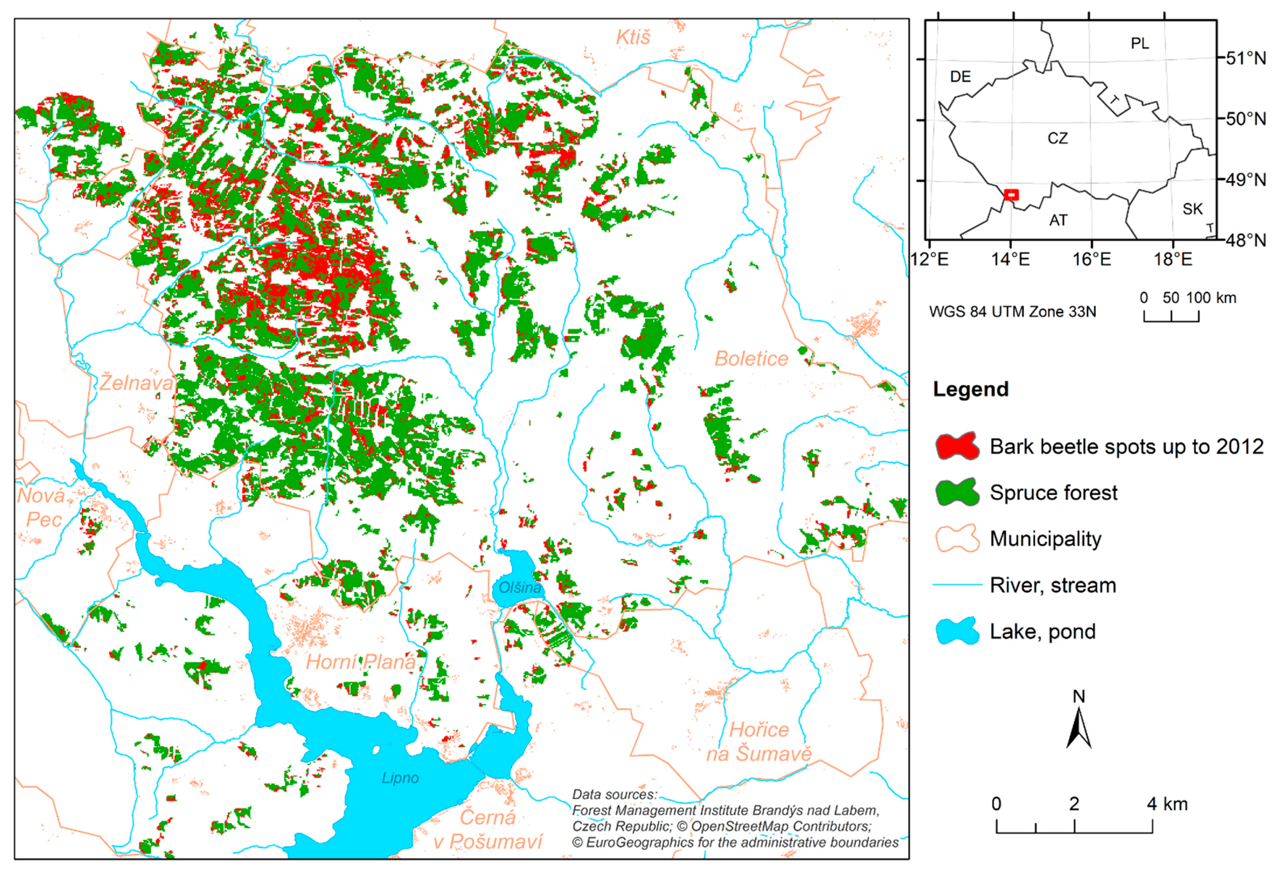
2.1. Study Area

MLAs were tested for the Horní Planá region in Central Europe (Figure 1). The forests in this region are managed by the Military Forests and Farms of the Czech Republic, State Enterprise [23]. The Military Forests and Farms of the Czech Republic, State Enterprise, is a special-purpose organization that manages 19,960 ha of land in military training areas. Forests represent 16,569 ha of this area, and water reservoirs cover 203 ha; the remaining area is represented by grassland that is used for intensive military training.

The region is characterized by hills that differ in elevation by 100–150 m. Most of the study area is located at 600 to 800 m a.s.l., and the highest point (Lysá Mt) is at 1228 m a.s.l. Part of the area belongs to the Bohemian Forest (the Šumava Mts.), and part belongs to the Šumavské podhůři Mts. The annual mean temperature ranges from 5 to 7 °C, and annual precipitation ranges from 700 to 800 mm [24].

The dominant tree species in forests is Norway spruce (Picea abies L. Karst) (69%). Less common are Scotch pine (Pinus sylvestris L.) (12%), Silver fir (Abies alba Mill.) (6%), and European beech (Fagus sylvatica L.) (5%). Among the forest stands, 23.5% are younger than 40 years, and 32.0% are older than 100 years. At higher altitudes, forests are parts of complexes that include meadows and pastures.

Spruce forests in the Horní Planá region are disturbed mainly by snow, bark beetles, and especially wind. In recent years, incidental felling caused by forest damage has represented about 50% of total felling. Bark beetle outbreaks in the region follow the trends exhibited over the whole of the Czech Republic, with peaks in the mid-1980s and mid-1990s. The last long-term outbreak of I. typographus began in 2003 as a result of a severe drought that occurred throughout Central Europe. This outbreak was partly extended by the winter storm “Kyrill” (January 2007), which destroyed more wood than any other factor over the last 30 years. At the beginning of 2014, the volume of wood infested by bark beetles decreased to under 0.5 m³·ha⁻¹ [25]. The cyclic nature of forest damage in the study region is depicted in Figure 2. The bark beetle is a prevailing cause of forest damage in the study region.

2.2. Input Data

In our study, spatial distribution models of spruce forest damage were developed for the period 2003–2012. The period was limited by years for which raster layers representing explanatory variables were available (

Table 1. List of the explanatory variables used in forest damage models (FDMs).

Code	Explanatory Variable
DAS	distance to forest damage spots from previous year
DFE	distance to spruce forest edge
PSR	potential global solar radiation
NDVI	normalized difference vegetation index
AGE	spruce forest age
PCT	percentage of spruce
VOL	volume of spruce wood per hectare
STO	stocking

). The spatial resolution of the raster layers was 30 m, which corresponds to the spatial resolution of LANDSAT images.

A time series of LANDSAT images were used to identify damaged forest locations in the study area. Raster maps of forest health status were used to delineate the damaged forest locations. These forest health maps are based on LANDSAT images and have been prepared by standardized methods since 1984 by the Forest Management Institute, Brandýs nad Labem, Czech Republic [26]. Forest damage locations were not classified by forest damage factors. Only classes of strong and very strong damage of spruce forest stands [27] were considered for this study. A similar approach was used by [28,29].

Normalized difference vegetation index (NDVI) values were derived from LANDSAT scenes (

Table 2. LANDSAT scenes used for NDVI calculation.

Date	Scene
16.07.2003	LT05_L1TP_191026_20030716_20161205_01_T1
10.08.2004	LT05_L1TP_192026_20040810_20161130_01_T1
28.07.2005 29.08.2005	LT05_L1TP_192026_20050728_20161125_01_T1 LT05_L1TP_192026_20050829_20161125_01_T1
15.07.2006 24.07.2006	LT05_L1TP_192026_20060715_20161120_01_T1 LT05_L1TP_191026_20060724_20161120_01_T1
25.06.2007 19.07.2007	LT05_L1TP_191026_20070625_20161112_01_T1 LE07_L1TP_191026_20070719_20170102_01_T1
29.06.2008 21.08.2008	LT05_L1TP_191026_20070625_20161112_01_T1 LT05_L1TP_192026_20080821_20180116_01_T1
24.08.2009	LT05_L1TP_192026_20090824_20161021_01_T1
10.07.2010	LT05_L1TP_192026_20100710_20161014_01_T1
23.08.2011	LT05_L1TP_191026_20110823_20161007_01_T1
23.07.2012 01.08.2012	LE07_L1TP_192026_20120723_20161130_01_T1 LE07_L1TP_191026_20120801_20161130_01_T1

). Cloud-free scenes from the growing season were preferred. Processing included manual removal of clouds and shadows and the mosaicking of two scenes based on linear regression using corresponding pixels that represented forest.

Information on spruce age (AGE), percentage of spruce in forest stands (PCT), volume of spruce per hectare (VOL), and stocking (STO) was imported from forest management plans. There are four management units within the study area, each with its own management plan. The forest management plans are prepared for 10-y periods. The age of a forest stand was specified in 5-year increments, and the percentage of spruce was based on basal area. Volume was derived from the stand mean diameter at breast height and the stand mean tree height for each species. Stocking was calculated as the relative density using yield tables. The raster layer representing spruce forest stands included only spruce stands with age >49 years and stocking >49%.

Distance to forest damage areas was calculated from the layer of actual forest damage. The actual forest damage layer was subtracted from the spruce forest stand layer to derive a layer of actual spruce forest. The raster layer of the actual spruce forest was used to calculate the distance to the spruce forest edge layer. Potential global solar radiation (PSR) was computed from a digital elevation model (DEM) by the GRASS GIS module r.sun [30] with a 1-h step.

EU-DEM 25 [31] was used as an input to compute PSR. Its original spatial resolution of 25 m is close to the resolution of LANDSAT scenes. The DEM was projected to the national spatial reference system (EPSG 5514, epsg.io/5514/) and resampled at a resolution of 30 m.

Samples representing damaged and undamaged forest were generated for each year of the period. All grid cells representing damaged forest were used as samples. An equal number of cells representing undamaged forest was randomly generated. Among the samples, 75% were used for model training, and 25% were used as controls. All FDMs were trained and validated using the same sample sets.

2.3. Computer Simulations and Data Processing

The FDM consists of a forest damage probability function and a classification function. The FDM $F$ can be expressed in the following form:

$$F\left(x,y,t\right)=C\left(P\left(\overrightarrow{u}\left(x,y,t\right)\right)\right)$$

(1)

where $C$ is a classification function; $P$ is a forest damage probability function; $\overrightarrow{u}$ is an environment vector function; x, y are point (grid cell) coordinates; and t is a time.

The probability function P calculates the risk of forest damage at a given location (x, y) and time t. Environmental factors, e.g., distance to existing forest damage areas, drought stress, forest stand openness, and solar radiation, are described by independent variables of the forest damage probability function P. Each component $u_i\left(x,y,t\right)$ of the environment vector function $\overrightarrow{u}$ corresponds to an independent variable that varies over space and time. In GIS, the independent variable is represented by a time series of raster layers.

The open source-software GRASS GIS [32] was used for computer simulations. All suitable MLAs from the GRASS GIS add-on r.learn.ml were tested for modeling the spatial distribution of forest damage (

Table 3. List of the tested machine learning algorithms (MLAs).

Code	Algorithm
LR	logistic regression
LDA	linear discriminant analysis
QDA	quadratic discriminant analysis
KNC	k-nearest neighbors classifier
GNB	Gaussian naive Bayes
DTC	decision tree classifier
RFC	random forest classifier
ETC	extra trees classifier
GBC	gradient boosting classifier
SVC	support vector classification

). r.learn.ml is a front-end to the scikit-learn toolkit [33] for the Python programming language. A set of scripts in Python programming language was developed to automate the processing of forest damage layers, the processing of training and control samples, model training, and the analysis of FDM performance.

In the study, the spatial distribution of forest damage was modeled by linear MLAs (LR and LDA), non-linear MLAs (QDA, KNC, GNB, and SVC), and classification trees (DTC, RFC, ETC, and GBC).

Each MLA was trained and tested on all subsets of the explanatory variables (Table 1). All combinations of explanatory variables were used as inputs of FDMs because the most suitable combinations of explanatory variables for different MLAs were unknown. The total number of FDMs tested was a product of the number of MLAs (10) × the number of combinations of exploratory variables (255). Each of the 2550 models was calculated for each year of the period 2003–2012. The probability of forest damage was calculated by each MLA. The internal classifier of each MLA was applied to identify locations (grid cells) of forest damage.

In a computer environment, a spatial forest damage model is defined by MLA m and a non-empty subset S of the explanatory variables. The forest damage spatial distribution model $fdm\left(m,S,y\right)$ was calculated for every year y of the period. The confusion matrix, true positive rate $TPR\left(m,S,y\right)$ true negative rate $TNR\left(m,S,y\right)$, and phi coefficient $\varphi \left(m,S,y\right)$ were calculated for each $fdm\left(m,S,y\right)$.

The true positive rate (sensitivity) describes how many locations (grid cells) of forest damage estimated by the FDM correspond to locations of actual forest damage. Similarly, the true negative rate (specificity) is a measure of the correspondence between estimated and actual undamaged forest locations. A reliable spatial FDM is characterized by high sensitivity and high specificity.

The overall performance of the spatial FDM was measured by the arithmetic mean of the phi coefficient for the period under study Y:

$$\overline{\Phi }\left(m,S\right)=\frac{1}{l}{\displaystyle \sum }_{y\in Y}\Phi \left(m,S,y\right),$$

(2)

where l is the length of the period Y, m is an used MLA, S is a non-empty subset of the explanatory variables, and y is a year of the period. The mean true positive rate $\overline{TPR}$(m,S) and the mean true negative rate $\overline{TNR}$(m,S) of the spatial FDM were calculated similarly.

Data were statistically processed with the R package [34]. All statistical hypotheses were tested at a 0.05 significance level. Modules from the packages lmPerm and RVAideMemoire were used for permutation tests of statistical hypotheses. Permutation one-way repeated measures ANOVA was used to compare the mean phi coefficients of the FDMs. Significances of mean phi coefficient differences were tested by a permutation pairwise t-test with Benjamini, Hochberg, and Yekutieli corrections [35].

The generated FDMs were sorted in descending order by $\overline{\varphi }$ (Equation (2)). A unique ranking number r was assigned to each FDM. The ranking number 1 corresponded to the FDM with the highest mean phi coefficient for the period Y. Results were evaluated in terms of FDM performance and simplicity.

3. Results

As stated earlier, the current study evaluated the use of MLAs for modeling the spatial distribution of forest damage. A simple spatial dispersion model was used (Equation (1)). The locations of damaged forest areas were modeled with the machine learning classifiers.

The top FDM (i.e., the FDM with the highest mean phi coefficient for the period 2003–2012) was selected for each studied MLA (

Table 4. Top FDMs generated by machine learning algorithms (MLAs).

r 1	nV 2	MLA 3	Variable 4								$\overline{\mathit{T}\mathit{P}\mathit{R}}{}^5$	$\overline{\mathit{T}\mathit{N}\mathit{R}}{}^6$	$\overline{\mathit{\varphi }}$7
			DAS	DFE	PSR	NDVI	AGE	PCT	VOL	STO
1	5	ETC	+		+		+	+	+		0.804	0.800	0.605
5	7	RFC	+	+	+		+	+	+	+	0.814	0.778	0.594
89	3	SVC					+	+	+		0.724	0.818	0.546
219	3	GBC					+	+	+		0.761	0.733	0.495
273	2	DTC					+		+		0.750	0.728	0.479
286	8	LDA	+	+	+	+	+	+	+	+	0.764	0.707	0.474
295	5	KNC	+	+			+	+	+		0.790	0.678	0.472
388	4	LR	+	+		+	+				0.769	0.679	0.452
421	7	QDA	+	+	+	+	+	+		+	0.815	0.618	0.444
436	5	GNB	+	+		+	+			+	0.827	0.602	0.441

¹ ranking number, ² number of explanatory variables, ³ machine learning algorithm used to generate FDM, the MLA codes are given in Table 3, ⁴ codes of the variables are listed in Table 1, ⁵ mean true positive rate, ⁶ mean true negative rate, ⁷ mean phi coefficient, “+” indicates the presence of an explanatory variable in FDM.

). As suspected, the optimal combination of input explanatory variables differed among the top FDMs.

The arithmetic mean and median of phi coefficients were higher for the top ETC-based model with five explanatory variables than for the other top FDMs for the period 2003–2012 (Table 4, Figure 3 and Figure 4). The influence of MLA on the mean phi coefficient ($\overline{\varphi }$) of the top FDMs was significant (one-way repeated measures ANOVA, p-value < 2.2×10−16). Results of the permutation pairwise t-test of the top FDMs’ $\varphi$ are presented in

Table 5. p-values of the pairwise permutation t-test of $\varphi$ of the top FDMs.

MLA 1	GNB	QDA	LR	KNC	LDA	DTC	GBC	SVC	RFC
QDA	0.827	-	-	-	-	-	-	-	-
LR	0.338	0.687	-	-	-	-	-	-	-
KNC	0.338	0.406	0.348	-	-	-	-	-	-
LDA	0.020	0.154	0.054	0.906	-	-	-	-	-
DTC	0.124	0.202	0.177	0.827	0.851	-	-	-	-
GBC	0.073	0.124	0.124	0.576	0.338	0.126	-	-	-
SVC	0.013	0.011	0.013	0.034	0.010	0.010	0.010	-	-
RFC	0.011	0.010	0.011	0.011	0.010	0.013	0.011	0.020	-
ETC	0.011	0.013	0.010	0.011	0.010	0.013	0.010	0.010	0.312

¹ the MLA codes are given in Table 3.

.

Overall performance as indicated by the mean phi coefficient was slightly lower for the best RFC-based model than for the best ETC-based model. However, performances for these best models were not significantly different. Performance for the other top FDM models was significantly different from performance for the best ETC- and RFC-based models (Table 5). Moreover, as evident in Figure 5, most of the ETC-based FDMs out-performed the FDMs generated by the other MLAs.

The performance of the FDMs generated by SVC was highly variable (Figure 5). SVC generated many low-performance FDMs as well as a few models that performed better than the models generated by the other tested MLAs except for those generated by ETC and RFC (Table 4). The performance of the best SVC-based model was significantly different from the performance of the other best FDMs (Table 5).

The mean TPRs were highest for the SVC-, QDA-, and GNB-based models (Figure 6). These models were highly sensitive because they significantly overestimated the area of damaged forest. On the other hand, SVC also generated several FDMs with low specificities (Figure 7).

We then compared the performance of the FDMs when the number of explanatory variables was constant in a range from one to eight. Regardless of the number of explanatory variables, performance was always best for the models generated by the ETC, RDC, and SVC MLAs (

Table 6. Top FDMs among models with equivalent numbers of explanatory variables.

r 1	nV 2	MLA 3	Variable 4								$\overline{\mathit{T}\mathit{P}\mathit{R}}{}^5$	$\overline{\mathit{T}\mathit{N}\mathit{R}}{}^6$	$\overline{\mathit{\varphi }}$7
			DAS	DFE	PSR	NDVI	AGE	PCT	VOL	STO
1055	1	SVC							+		0.691	0.685	0.376
116	2	SVC					+		+		0.719	0.811	0.534
43	3	RFC	+				+		+		0.794	0.773	0.568
16	4	ETC	+		+		+		+		0.800	0.784	0.585
1	5	ETC	+		+		+	+	+		0.804	0.800	0.605
6	6	ETC	+		+	+	+	+	+		0.791	0.800	0.592
2	7	ETC	+		+	+	+	+	+	+	0.793	0.806	0.600
3	8	ETC	+	+	+	+	+	+	+	+	0.804	0.790	0.596

¹ ranking number, ² number of explanatory variables, ³ machine learning algorithm used to generate FDM, the MLA codes are given in Table 3, ⁴ codes of the variables are listed in Table 1, ⁵ mean true positive rate, ⁶ mean true negative rate, ⁷ mean phi coefficient, “+” indicates the presence of an explanatory variable in FDM.

). Performance of FDMs generated by most of the MLAs increased with the number of variables, except in the case of SVC- and KNC-based models (Appendix A).

The Φ of ETC-based models generally increased as the number of explanatory variables increased (Figure A1). The computer simulations showed that the ETC-based model that included distance to actual forest damage, potential solar radiation, spruce forest age, percentage of spruce in forest stands, and volume per hectare had the highest mean accuracy and phi coefficient. Nearly the same performance, however, was achieved by ETC-based models that included different explanatory variables (

Table A1. Forest damage models not significantly different from the best ETC-based model.

r 1	nV 2	MLA 3	Variable 4								$\overline{\mathit{T}\mathit{P}\mathit{R}}{}^5$	$\overline{\mathit{T}\mathit{N}\mathit{R}}{}^6$	$\overline{\mathit{\varphi }}$7	p 8
			DAS	DFE	PSR	NDVI	AGE	PCT	VOL	STO
1	ETC	5	+		+		+	+	+		0.8043	0.8002	0.6052	-
2	ETC	7	+		+	+	+	+	+	+	0.7927	0.8058	0.5997	0.5537
3	ETC	8	+	+	+	+	+	+	+	+	0.8038	0.7905	0.5959	0.5037
4	ETC	7	+	+	+		+	+	+	+	0.8045	0.7898	0.5957	0.4998
5	RFC	7	+	+	+		+	+	+	+	0.8140	0.7782	0.5937	0.2509
6	ETC	6	+		+	+	+	+	+		0.7910	0.8001	0.5919	0.1819
7	ETC	5	+		+		+		+	+	0.8035	0.7856	0.5902	0.1029
8	ETC	6	+	+	+		+	+	+		0.8103	0.7782	0.5898	0.2369
9	ETC	7	+	+		+	+	+	+	+	0.7989	0.7890	0.5897	0.2859
10	ETC	7	+	+	+	+	+	+		+	0.8004	0.7869	0.5896	0.1759
12	ETC	6	+		+	+		+	+	+	0.7807	0.8069	0.5888	0.1829
13	RFC	6	+	+	+		+		+	+	0.8036	0.7833	0.5882	0.0770
14	ETC	7	+	+	+	+	+	+	+		0.7980	0.7882	0.5877	0.1479
16	ETC	4	+		+		+		+		0.8004	0.7844	0.5855	0.0800
18	ETC	6	+		+	+	+		+	+	0.7813	0.8027	0.5851	0.0860
21	ETC	6	+	+	+		+		+	+	0.7983	0.7787	0.5783	0.0820
36	ETC	7	+	+	+	+		+	+	+	0.7881	0.7798	0.5693	0.0510

¹ ranking number, ² number of explanatory variables, ³ machine learning algorithm used to generate FDM, the MLA codes are given in Table 3, ⁴ codes of the variables are listed in Table 1, ⁵ mean true positive rate, ⁶ mean true negative rate, ⁷ mean phi coefficient for the period 2003–2012, ⁸ p-value of pairwise permutation t-test with the best model, “+” indicates the presence of an explanatory variable in FDM.

).

4. Discussion

Given climate change and the increased emphasis on ecological and cultural services rather than on the economic services provided by forest ecosystems, new forest management strategies are needed. Forest damage by abiotic and biotic factors not only causes timber loss, but also has negative effects in terms of forest diversity, soil erosion, landslides, recreation, and landscape aesthetics. The spatial pattern of forest damage is driven by complex spatio-temporal environmental processes. Rammer and Seidl [36] have shown the effectiveness of MLAs for the spatial prediction of I. typographus infestations in unmanaged forests.

We found that FDMs based on traditional linear and non-linear methods generally performed less well than FDMs based on classification trees. LR and LDA are commonly used linear classification MLAs. Hernandez et al. [37] developed a spatial logistic regression model of the probability of bark beetle (Dendroctonus frontalis Zimmermann) attack in coniferous forests; the overall accuracy of the model was 68.7%. LR, which is a special case of the generalized linear model, models the log-odds as a linear function by minimizing the sum of the squared residuals. LDA minimizes the probability of misclassification by maximizing the separation between the classes. LR and LDA create the linear boundaries of classes in the explanatory variables’ space. LDA is less sensitive than LR to correlations between explanatory variables.

QDA uses class-specific covariance matrices and separates classes by quadratic surfaces in the predictors’ space. It is sensitive to collinearity between explanatory variables within a class. Because of a higher complexity of the discriminant function, QDA may perform better than linear MLAs. KNC calculates class probability as the proportion of the class in the set of k-closest neighbors from the training data. KNC is susceptible to measurement scales and local over-fitting. GNB estimates prior and conditional probabilities from the training set and then uses Bayes’s rule to calculate the probability of outcome class. An important assumption of GNB is the independence of explanatory variables, which is rarely satisfied in practice.

Only the performance of the top SVC-based FDM was significantly different from the best models generated by the other tested linear and non-linear algorithms. SVC is considered one of the most flexible and effective MLAs and is widely used. It belongs to the family of kernel methods, which allow the separation of classes by non-linear boundaries.

In our study, the FDMs generated by classification trees performed better than those generated by linear and non-linear MLAs. Classification trees describe patterns in data by complex hierarchies of simple rules. The performance of a single classification tree is usually weak. The performances of DTC-based FDMs were inferior to those of the FDMs generated by MLAs based on an ensemble of classification trees.

An ensemble of classification trees usually performs better than a single classification tree, because an ensemble can detect more complex patterns in the data. The RFC MLA is an ensemble of classification trees that are trained on bootstrap samples. The randomness of the tree construction process reduces correlations between trees. Mi et al. [38] investigated Stochastic Gradient Boosting, RFC, CART (Classification and Regression Tree), and MaxEnt (Maximum Entropy) for the modeling distribution of three crane species. The RFC-generated species distribution models were found more reliable and accurate than models generated by the other algorithms under their study.

The process of GBC ensemble construction is iterative. The newly constructed classification tree of the GBC ensemble is forced to learn unexplored data. However, the boosting process was not effective in the case of FDMs. In our study, GBC-based FDMs performed less well than the RFC- and ETC-based models.

The best results in our study were achieved by FDMs generated by ETC. In the ETC ensemble, classification trees are trained on all samples. The randomly selected exploratory variable and random value are used to split the nodes of the classification trees [39]. ETC-based models were responsive to the spatial variance of environmental conditions, they accurately modeled the spatial distribution of forest damage. In addition, ETC-based models are computationally efficient.

Default settings were used for testing the MLAs in the current study. These default settings were selected by developers based on their knowledge of algorithms. Although these settings provide a good starting point for experiments with MLAs, optimization of settings may improve the performance of the tested algorithms.

Input variables for FDMs vary over space and time. Field measurements and access to historical records or remote sensing data are needed to prepare corresponding inputs for spatial distribution models. PSR, NDVI, and distance to existing forest damage areas can be calculated for past periods. Archives of satellite images can be used to calculate NDVI and to identify bark beetle infestations for past years. Thanks to the archiving of satellite images, it should be possible to identify past and current infestations and to build spatial distribution models that predict future forest damage.

We tested all combinations of the explanatory variables as input to the studied MLAs. However, only eight explanatory variables were available for our study area (Table 1). As indicated in Table 4 and Table A1, some explanatory variables occurred more often than other explanatory variables in FDMs. The most common explanatory variables in the top FDMs were distance to damaged forest, potential solar radiation, forest age, and spruce volume per hectare (Table A1). These variables may carry substantial information for modeling the spatial distribution of forest damage [40,41,42,43].

5. Conclusions

In the study, we evaluated the performance of 10 MLAs and combinations of eight input variables for the spatial modeling of spruce forest damage. Our computer simulations confirmed the suitability of the ETC MLA for modeling the spatial distribution of spruce forest damage. We also found that the number of input explanatory variables could be reduced without significant spatial modeling accuracy loss. A smaller number of input explanatory variables simplifies data preparation and processing and therefore reduces financial costs.

Various MLAs are currently ready for use in spatial decision support systems. We evaluated the MLAs available in the open-source GRASS GIS. The identification of suitable MLAs and key environmental variables is an essential step in the development of GIS tools for forest damage modeling and prognosis. Our findings will facilitate the development of the open-source spatial decision system TANABBO for modeling the spatial distribution of forest damage related to I. typographus.

The risk of forest damage is affected by many interrelated environmental factors, forest stand parameters, and forest management practices. MLAs are effective for modeling non-linear, complex phenomena like the spatial distribution of forest damage. This study provides researchers and forest managers with an accurate method of modeling spatial forest damage. The integration of the FDM with a spatial decision support system will facilitate novel tools for managing forests.

References

1. Brázdil, R.; Stucki, P.; Szabó, P.; Řezníčková, L.; Dolák, L.; Dobrovolný, P.; Tolasz, R.; Kotyza, O.; Chromá, K.; Suchánková, S. Windstorms and Forest Disturbances in the Czech Lands: 1801–2015. Agric. For. Meteorol. 2018, 250–251, 47–63. [Google Scholar] [CrossRef]
2. Mezei, P.; Grodzki, W.; Blaženec, M.; Jakuš, R. Factors Influencing the Wind–Bark Beetles’ Disturbance System in the Course of an Ips Typographus Outbreak in the Tatra Mountains. For. Ecol. Manag. 2014, 312, 67–77. [Google Scholar] [CrossRef]
3. Seidl, R.; Thom, D.; Kautz, M.; Martin-Benito, D.; Peltoniemi, M.; Vacchiano, G.; Wild, J.; Ascoli, D.; Petr, M.; Honkaniemi, J.; et al. Forest Disturbances under Climate Change. Nat. Clim. Change 2017, 7, 395–402. [Google Scholar] [CrossRef] [Green Version]
4. Schurman, J.S.; Trotsiuk, V.; Bače, R.; Čada, V.; Fraver, S.; Janda, P.; Kulakowski, D.; Labusova, J.; Mikoláš, M.; Nagel, T.A.; et al. Large-Scale Disturbance Legacies and the Climate Sensitivity of Primary Picea Abies Forests. Glob. Chang. Biol. 2018, 24, 2169–2181. [Google Scholar] [CrossRef] [PubMed]
5. Mezei, P.; Jakuš, R.; Pennerstorfer, J.; Havašová, M.; Škvarenina, J.; Ferenčík, J.; Slivinský, J.; Bičárová, S.; Bilčík, D.; Blaženec, M.; et al. Storms, Temperature Maxima and the Eurasian Spruce Bark Beetle Ips Typographus—An Infernal Trio in Norway Spruce Forests of the Central European High Tatra Mountains. Agric. For. Meteorol. 2017, 242, 85–95. [Google Scholar] [CrossRef]
6. Montano, V.; Bertheau, C.; Doležal, P.; Krumböck, S.; Okrouhlík, J.; Stauffer, C.; Moodley, Y. How Differential Management Strategies Affect Ips Typographus L. Dispersal. For. Ecol. Manag. 2016, 360, 195–204. [Google Scholar] [CrossRef]
7. Lausch, A.; Heurich, M.; Fahse, L. Spatio-Temporal Infestation Patterns of Ips Typographus (L.) in the Bavarian Forest National Park, Germany. Ecol. Indic. 2013, 31, 73–81. [Google Scholar] [CrossRef]
8. Økland, B.; Nikolov, C.; Krokene, P.; Vakula, J. Transition from Windfall- to Patch-Driven Outbreak Dynamics of the Spruce Bark Beetle Ips Typographus. For. Ecol. Manag. 2016, 363, 63–73. [Google Scholar] [CrossRef]
9. de Groot, M.; Ogris, N. Short-Term Forecasting of Bark Beetle Outbreaks on Two Economically Important Conifer Tree Species. For. Ecol. Manag. 2019, 450, 117495. [Google Scholar] [CrossRef]
10. Segura, M.; Ray, D.; Maroto, C. Decision Support Systems for Forest Management: A Comparative Analysis and Assessment. Comput. Electron. Agric. 2014, 101, 55–67. [Google Scholar] [CrossRef]
11. Senf, C.; Seidl, R.; Hostert, P. Remote Sensing of Forest Insect Disturbances: Current State and Future Directions. Int. J. Appl. Earth Obs. Geoinf. 2017, 60, 49–60. [Google Scholar] [CrossRef] [PubMed] [Green Version]
12. Oeser, J.; Pflugmacher, D.; Senf, C.; Heurich, M.; Hostert, P. Using Intra-Annual Landsat Time Series for Attributing Forest Disturbance Agents in Central Europe. Forests 2017, 8, 251. [Google Scholar] [CrossRef]
13. Thiele, J.C.; Nuske, R.S.; Ahrends, B.; Panferov, O.; Albert, M.; Staupendahl, K.; Junghans, U.; Jansen, M.; Saborowski, J. Climate Change Impact Assessment—A Simulation Experiment with Norway Spruce for a Forest District in Central Europe. Ecol. Model. 2017, 346, 30–47. [Google Scholar] [CrossRef]
14. Seidl, R.; Müller, J.; Hothorn, T.; Bässler, C.; Heurich, M.; Kautz, M. Small Beetle, Large-Scale Drivers: How Regional and Landscape Factors Affect Outbreaks of the European Spruce Bark Beetle. J. Appl. Ecol. 2016, 53, 530–540. [Google Scholar] [CrossRef]
15. dos Reis, A.A.; Carvalho, M.C.; de Mello, J.M.; Gomide, L.R.; Ferraz Filho, A.C.; Acerbi Junior, F.W. Spatial Prediction of Basal Area and Volume in Eucalyptus Stands Using Landsat TM Data: An Assessment of Prediction Methods. N. Z. J. For. Sci. 2018, 48. [Google Scholar] [CrossRef] [Green Version]
16. Hickey, C.; Kelly, S.; Carroll, P.; O’Connor, J. Prediction of Forestry Planned End Products Using Dirichlet Regression and Neural Networks. For. Sci. 2015, 61, 289–297. [Google Scholar] [CrossRef] [Green Version]
17. Görgens, E.B.; Montaghi, A.; Rodriguez, L.C.E. A Performance Comparison of Machine Learning Methods to Estimate the Fast-Growing Forest Plantation Yield Based on Laser Scanning Metrics. Comput. Electron. Agric. 2015, 116, 221–227. [Google Scholar] [CrossRef]
18. Rodrigues, M.; de la Riva, J. An Insight into Machine-Learning Algorithms to Model Human-Caused Wildfire Occurrence. Environ. Model. Softw. 2014, 57, 192–201. [Google Scholar] [CrossRef]
19. Mayfield, H.; Smith, C.; Gallagher, M.; Hockings, M. Use of Freely Available Datasets and Machine Learning Methods in Predicting Deforestation. Environ. Model. Softw. 2017, 87, 17–28. [Google Scholar] [CrossRef] [Green Version]
20. Castelli, M.; Vanneschi, L.; Popovič, A. Predicting Burned Areas of Forest Fires: An Artificial Intelligence Approach. Fire Ecol. 2015, 11, 106–118. [Google Scholar] [CrossRef]
21. Liang, L.; Li, X.; Huang, Y.; Qin, Y.; Huang, H. Integrating Remote Sensing, GIS and Dynamic Models for Landscape-Level Simulation of Forest Insect Disturbance. Ecol. Model. 2017, 354, 1–10. [Google Scholar] [CrossRef] [Green Version]
22. Hlásny, T.; Turčáni, M. Persisting Bark Beetle Outbreak Indicates the Unsustainability of Secondary Norway Spruce Forests: Case Study from Central Europe. Ann. For. Sci. 2013, 70, 481–491. [Google Scholar] [CrossRef] [Green Version]
23. Military Forests and Farms of the Czech Republic, State Enterprise. Available online: https://www.vls.cz/en (accessed on 25 March 2021).
24. Culek, M.; Grulich, V.; Laštůvka, Z.; Divíšek, J. Biogeografické Regiony České Republiky; Masarykova Univerzita: Brno, Czech Republic, 2013; ISBN 978-80-210-6693-9. [Google Scholar]
25. Forestry and Game Management Research Institute, Czech Republic. Available online: https://www.vulhm.cz/en/ (accessed on 25 March 2021).
26. Forest Management Institute (FMI), Czech Republic. Available online: http://www.uhul.cz/home (accessed on 25 March 2021).
27. Henzlik, V. Forests and Air Pollution in the Czech Republic. In Restoration of Forests; Gutkowski, R.M., Winnicki, T., Eds.; Springer Netherlands: Dordrecht, The Netherlands, 1997; pp. 133–149. ISBN 978-0-7923-4634-0. [Google Scholar]
28. Havašová, M.; Ferenčík, J.; Jakuš, R. Interactions between Windthrow, Bark Beetles and Forest Management in the Tatra National Parks. For. Ecol. Manag. 2017, 391, 349–361. [Google Scholar] [CrossRef]
29. Ďuračiová, R.; Muňko, M.; Barka, I.; Koreň, M.; Resnerová, K.; Holuša, J.; Blaženec, M.; Potterf, M.; Jakuš, R. A Bark Beetle Infestation Predictive Model Based on Satellite Data in the Frame of Decision Support System TANABBO. IForest Biogeosci. For. 2020, 13, 215–223. [Google Scholar] [CrossRef]
30. Hofierka, J.; Šúri, M. The Solar Radiation Model for Open Source GIS: Implementation and Applications. In Proceedings of the Open Source GIS—GRASS Users Conference 2002, Trento, Italy, 11–13 September 2002; p. 19. [Google Scholar]
31. EU-DEM v1.1—Copernicus Land Monitoring Service. Available online: https://land.copernicus.eu/imagery-in-situ/eu-dem/eu-dem-v1.1 (accessed on 25 March 2021).
32. GRASS GIS. Available online: https://grass.osgeo.org/ (accessed on 25 March 2021).
33. Scikit-Learn: Machine Learning in Python. Available online: https://scikit-learn.org (accessed on 25 March 2021).
34. R Core Team R: A Language and Environment for Statistical Computing; R Foundation for Statistical Computing: Vienna, Austria, 2018.
35. Benjamini, Y.; Hochberg, Y. Controlling the False Discovery Rate: A Practical and Powerful Approach to Multiple Testing. J. R. Stat. Soc. Ser. B Methodol. 1995, 57, 289–300. [Google Scholar] [CrossRef]
36. Rammer, W.; Seidl, R. Harnessing Deep Learning in Ecology: An Example Predicting Bark Beetle Outbreaks. Front. Plant Sci. 2019, 10, 1327. [Google Scholar] [CrossRef] [PubMed]
37. Hernandez, A.J.; Saborio, J.; Ramsey, R.D.; Rivera, S. Likelihood of Occurrence of Bark Beetle Attacks on Conifer Forests in Honduras under Normal and Climate Change Scenarios. Geocarto Int. 2012, 27, 581–592. [Google Scholar] [CrossRef]
38. Mi, C.; Huettmann, F.; Guo, Y.; Han, X.; Wen, L. Why Choose Random Forest to Predict Rare Species Distribution with Few Samples in Large Undersampled Areas? Three Asian Crane Species Models Provide Supporting Evidence. PeerJ 2017, 5, e2849. [Google Scholar] [CrossRef] [PubMed] [Green Version]
39. Geurts, P.; Ernst, D.; Wehenkel, L. Extremely Randomized Trees. Mach. Learn. 2006, 63, 3–42. [Google Scholar] [CrossRef] [Green Version]
40. Angst, A.; Rüegg, R.; Forster, B. Declining Bark Beetle Densities (Ips Typographus, Coleoptera: Scolytinae) from Infested Norway Spruce Stands and Possible Implications for Management. Psyche J. Entomol. 2012, 2012, 1–7. [Google Scholar] [CrossRef]
41. Kautz, M.; Schopf, R.; Ohser, J. The “Sun-Effect”: Microclimatic Alterations Predispose Forest Edges to Bark Beetle Infestations. Eur. J. For. Res. 2013, 132, 453–465. [Google Scholar] [CrossRef]
42. Stadelmann, G.; Bugmann, H.; Wermelinger, B.; Meier, F.; Bigler, C. A Predictive Framework to Assess Spatio-Temporal Variability of Infestations by the European Spruce Bark Beetle. Ecography 2013, 36, 1208–1217. [Google Scholar] [CrossRef]
43. Stereńczak, K.; Mielcarek, M.; Kamińska, A.; Kraszewski, B.; Piasecka, Ż.; Miścicki, S.; Heurich, M. Influence of Selected Habitat and Stand Factors on Bark Beetle Ips Typographus (L.) Outbreak in the Białowieża Forest. For. Ecol. Manag. 2020, 459, 117826. [Google Scholar] [CrossRef]
Figure 1. Location of the study area in the Czech Republic.
Forests 12 00395 g001
Figure 2. Size of forest damaged areas in the study region (calculated from classified LANDSAT images).
Forests 12 00395 g002
Figure 3. Boxplot of phi coefficients ( ϕ ) of the top FDMs generated by MLAs. Box plots show median plus upper and lower quartiles of the phi coefficient for the period 2003–2012. Minimum and maximum values are indicated by the upper and lower whiskers (1.5 × interquartile range). Circles are outliers. The MLA codes are given in Table 3.
Forests 12 00395 g003
Figure 4. Preview of the bark beetle spots generated by the top ETC-based model. Green color represents unaffected spruce forest; blue color represents bark beetle infestation spots generated by the top ETC-based model; red color represents damaged forest identified on LANDSAT images. The MLA codes are given in Table 3, and the variables of the top models are listed in Table 4.
Forests 12 00395 g004
Figure 5. Box plots of mean phi coefficients ( ϕ ¯ ) of FDMs generated by MLAs. Box plots show median plus upper and lower quartiles for mean phi coefficients of all FDMs generated by a given algorithm. Minimum and maximum values are indicated by the upper and lower whiskers (1.5 × interquartile range). Circles are outliers. See Table 3 for MLA codes.
Forests 12 00395 g005
Figure 6. Box plots of mean sensitivities ( T P R ¯ ) of FDMs generated by MLAs. Box plots show median plus upper and lower quartiles for mean sensitivities of all FDMs generated by a given algorithm. Minimum and maximum values are indicated by the upper and lower whiskers (1.5 × interquartile range). Circles are outliers. See Table 3 for MLA codes.
Forests 12 00395 g006
Figure 7. Box plots of mean specificities ( T N R ¯ ) of FDMs generated by MLAs. Box plots show median plus upper and lower quartiles for mean specificities of all FDMs generated by a given algorithm. Minimum and maximum values are indicated by the upper and lower whiskers (1.5 × interquartile range). Circles are outliers. See Table 3 for MLA codes.
Forests 12 00395 g007