
A Deep Learning Approach to Downscale Geostationary Satellite Imagery for Decision Support in High Impact Wildfires

 , , and
Abstract
1. Introduction
2. Methodology
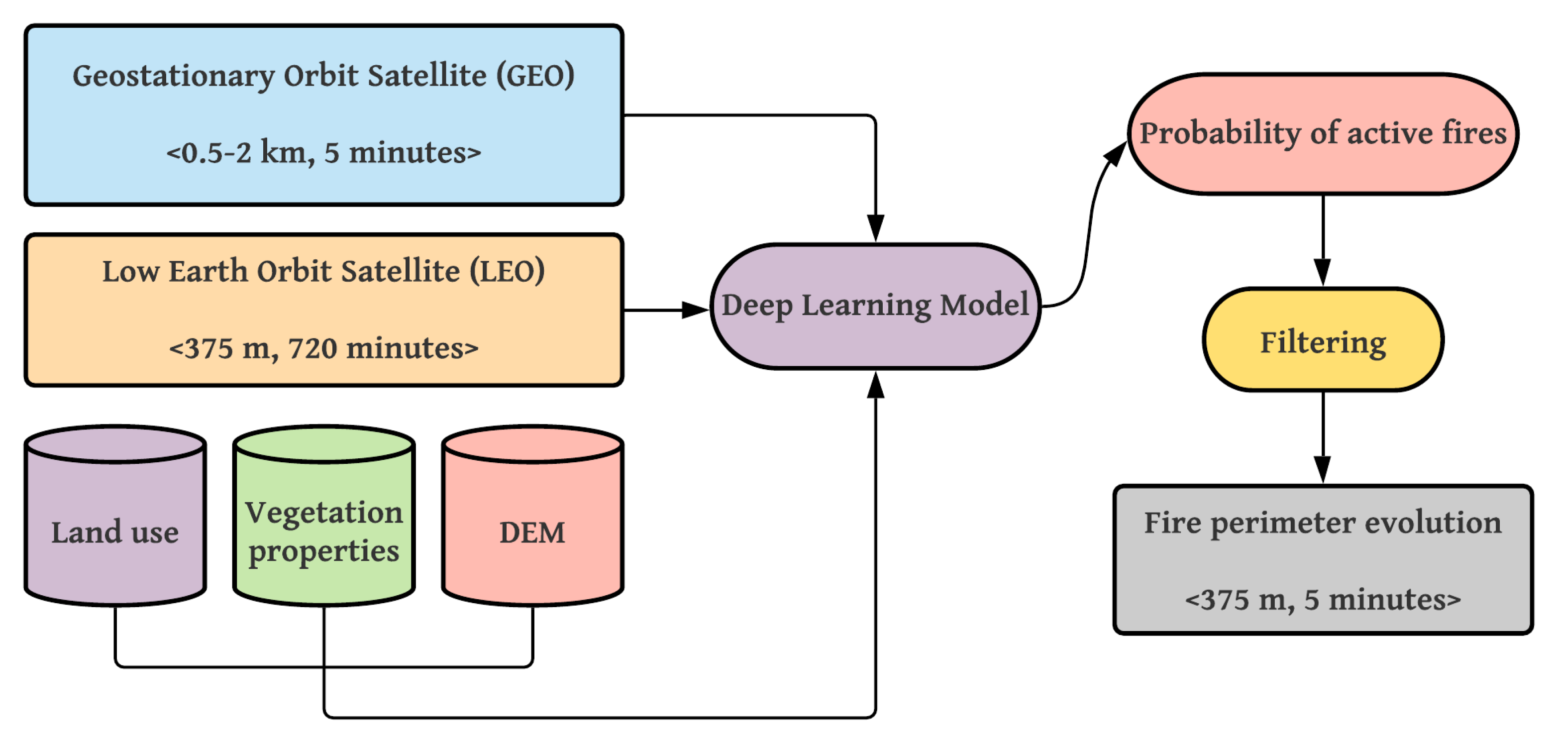
2.1. Input Data
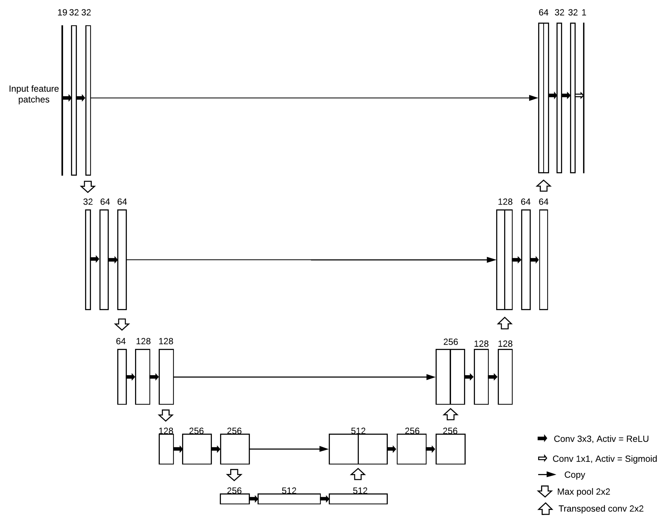
2.2. Deep Learning Model Architecture
2.3. Pre-Processing and Feature Engineering
2.4. Model Training
2.5. Post-Processing
3. Operational Implementation
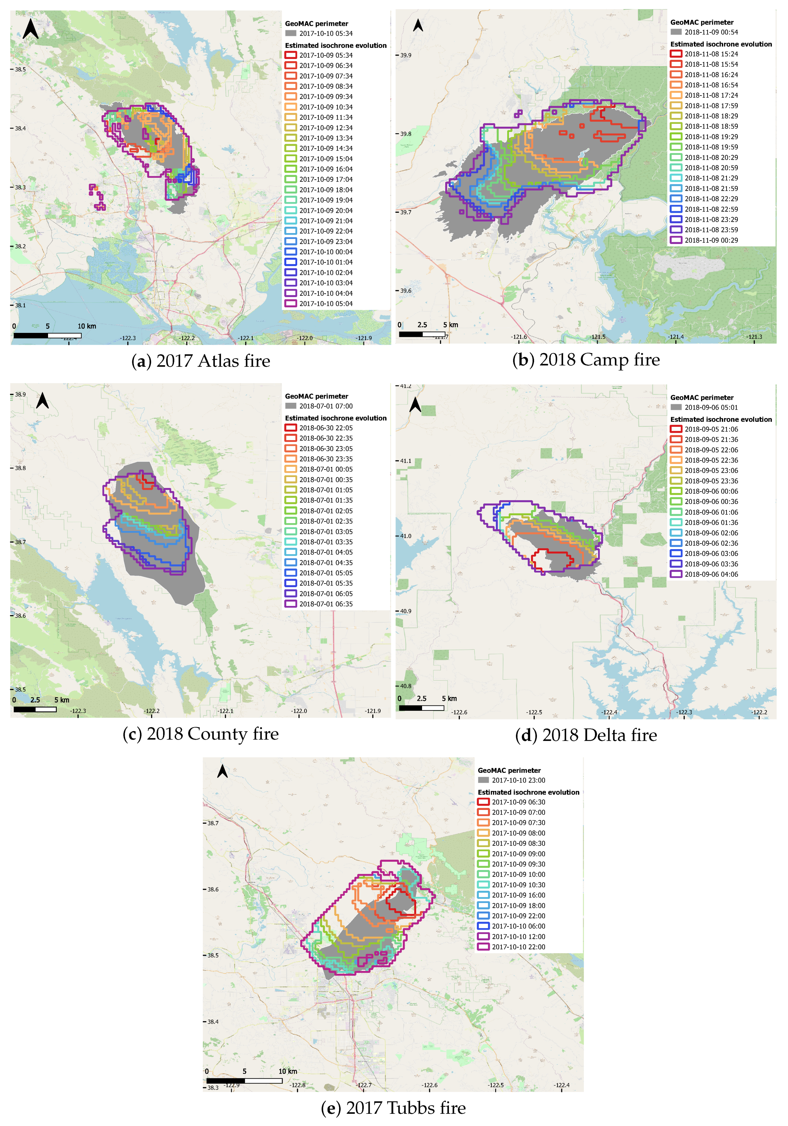
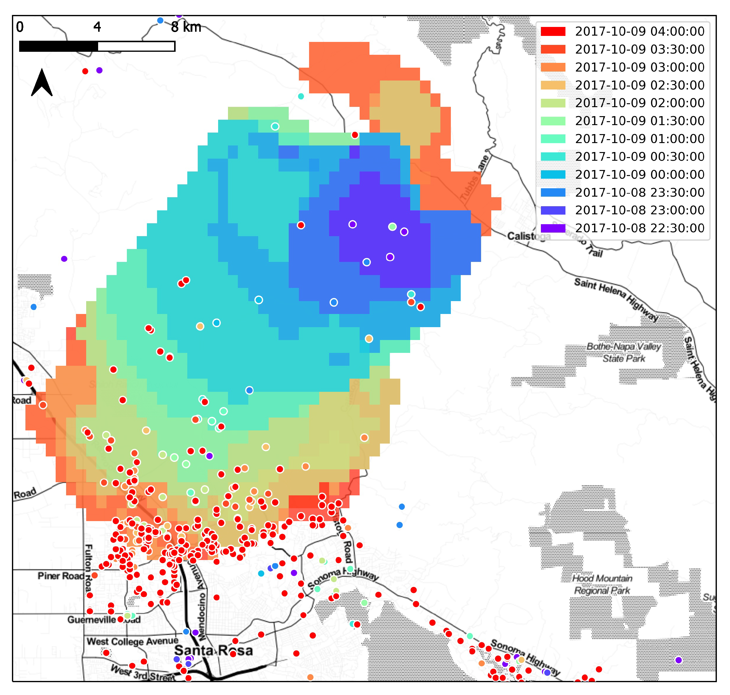
4. Validation

5. Discussion, Conclusions and Future Work
Author Contributions
Funding
Institutional Review Board Statement
Informed Consent Statement
Data Availability Statement
Acknowledgments
Conflicts of Interest
References
- Bowman, D.M.J.S.; Williamson, G.J.; Abatzoglou, J.T.; Kolden, C.A.; Cochrane, M.A.; Smith, A.M.S. Human exposure and sensitivity to globally extreme wildfire events. Nat. Ecol. Evol. 2017, 1, 0058. [Google Scholar] [CrossRef] [PubMed]
- Calkin, D.E.; Cohen, J.D.; Finney, M.A.; Thompson, M.P. How risk management can prevent future wildfire disasters in the wildland–urban interface. Proc. Natl. Acad. Sci. USA 2014, 111, 746–751. [Google Scholar] [CrossRef] [PubMed]
- Berlin, G.; Hieb, M. Wildland Urban Interface Fire Operational Requirements and Capability Analysis—Report of Findings; Technical Report; US Department of Homeland Security, Science and Technology Directorate. 2019. Available online: https://www.dhs.gov/publication/st-wui-fire-operational-requirements-and-capability-analysis-report-findings (accessed on 2 March 2021).
- Duff, T.J.; Chonga, D.M.; Cirulisa, B.A.; Walsha, S.F.; Penmanb, T.D.; Tolhust, K.G. Gaining benefits from adversity: The need for systems and frameworks to maximise the data obtained from wildfires. In Advances in Forest Fire Research; Viegas, D.X., Ed.; Imprensa da Universidade de Coimbra: Coimbra, Portugal, 2014; pp. 766–774. [Google Scholar] [CrossRef]
- Filkov, A.I.; Duff, T.J.; Penman, T.D. Improving fire behaviour data obtained from wildfires. Forests 2018, 9, 81. [Google Scholar] [CrossRef]
- Finney, M.A.; Cohen, J.D.; McAllister, S.S.; Jolly, W.M. On the need for a theory of wildland fire spread. Int. J. Wildland Fire 2013, 22, 25–36. [Google Scholar] [CrossRef]
- Cruz, M.G.; Alexander, M.E. Uncertainty associated with model predictions of surface and crown fire rates of spread. Environ. Model. Softw. 2013, 47, 16–28. [Google Scholar] [CrossRef]
- Cruz, M.G.; Sullivan, A.L.; Gould, J.S.; Hurley, R.J.; Plucinski, M.P. Got to burn to learn: The effect of fuel load on grassland fire behaviour and its management implications. Int. J. Ofwildland Fire 2018, 27, 727–741. [Google Scholar] [CrossRef]
- Bachmann, A.; Allöwer, B. Uncertainty propagation in wildland fire behaviour modelling. Int. J. Geogr. Inf. Sci. 2002, 16, 115–127. [Google Scholar] [CrossRef]
- Monedero, S.; Ramirez, J.; Molina-Terrén, D.; Cardil, A. Simulating wildfires backwards in time from the final fire perimeter in point-functional fire models. Environ. Model. Softw. 2017, 92, 163–168. [Google Scholar] [CrossRef]
- Mandel, J.; Bennethum, L.S.; Beezley, J.D.; Coen, J.L.; Douglas, C.C.; Kim, M.; Vodacek, A. A wildland fire model with data assimilation. Math. Comput. Simul. 2008, 79, 584–606. [Google Scholar] [CrossRef]
- Rios, O.; Jahn, W.; Rein, G. Forecasting wind-driven wildfires using an inverse modelling approach. Nat. Hazards Earth Syst. Sci. 2014, 14, 1491–1503. [Google Scholar] [CrossRef]
- Rios, O.; Pastor, E.; Valero, M.M.; Planas, E. Short-term fire front spread prediction using inverse modelling and airborne infrared images. Int. J. Wildland Fire 2016, 25, 1033–1047. [Google Scholar] [CrossRef][Green Version]
- Rios, O.; Valero, M.M.; Pastor, E.; Planas, E. A Data-Driven Fire Spread Simulator: Validation in Vall-llobrega’s Fire. Front. Mech. Eng. 2019, 5. [Google Scholar] [CrossRef]
- Rochoux, M.C.; Ricci, S.; Lucor, D.; Cuenot, B.; Trouvé, A. Towards predictive data-driven simulations of wildfire spread—Part I: Reduced-cost ensemble Kalman filter based on a polynomial chaos surrogate model for parameter estimation. Nat. Hazards Earth Syst. Sci. 2014, 14, 2951–2973. [Google Scholar] [CrossRef]
- Rochoux, M.C.; Emery, C.; Ricci, S.; Cuenot, B.; Trouvé, A. Towards predictive data-driven simulations of wildfire spread—Part II: Ensemble Kalman Filter for the state estimation of a front-tracking simulator of wildfire spread. Nat. Hazards Earth Syst. Sci. 2015, 15, 1721–1739. [Google Scholar] [CrossRef]
- Valero, M.M.; Jimenez, D.; Butler, B.W.; Mata, C.; Rios, O.; Pastor, E.; Planas, E. On the use of compact thermal cameras for quantitative wildfire monitoring. In Advances in Forest Fire Research 2018; Viegas, D.X., Ed.; University of Coimbra Press: Coimbra, Portugal, 2018; Chapter 5; pp. 1077–1086. [Google Scholar] [CrossRef]
- Lentile, L.B.; Holden, Z.A.; Smith, A.M.S.; Falkowski, M.J.; Hudak, A.T.; Morgan, P.; Lewis, S.A.; Gessler, P.E.; Benson, N.C. Remote sensing techniques to assess active fire characteristics and post-fire effects. Int. J. Wildland Fire 2006, 15, 319. [Google Scholar] [CrossRef]
- Ichoku, C.; Kahn, R.; Chin, M. Satellite contributions to the quantitative characterization of biomass burning for climate modeling. Atmos. Res. 2012, 111, 1–28. [Google Scholar] [CrossRef]
- Weaver, J.F.; Lindsey, D.; Bikos, D.; Schmidt, C.C.; Prins, E. Fire detection using GOES rapid scan imagery. Weather Forecast. 2004, 19, 496–510. [Google Scholar] [CrossRef]
- Smith, A.M.; Wooster, M.J. Remote classification of head and backfire types from MODIS fire radiative power and smoke plume observations. Int. J. Wildland Fire 2005, 14, 249–254. [Google Scholar] [CrossRef]
- Koltunov, A.; Ustin, S.L.; Prins, E.M. On timeliness and accuracy of wildfire detection by the GOES WF-ABBA algorithm over California during the 2006 fire season. Remote Sens. Environ. 2012, 127, 194–209. [Google Scholar] [CrossRef]
- Oliva, P.; Schroeder, W. Assessment of VIIRS 375m active fire detection product for direct burned area mapping. Remote Sens. Environ. 2015, 160, 144–155. [Google Scholar] [CrossRef]
- Schroeder, W.; Oliva, P.; Giglio, L.; Quayle, B.; Lorenz, E.; Morelli, F. Active fire detection using Landsat-8/OLI data. Remote Sens. Environ. 2016, 185, 210–220. [Google Scholar] [CrossRef]
- Liu, X.; He, B.; Quan, X.; Yebra, M.; Qiu, S.; Yin, C.; Liao, Z.; Zhang, H. Near real-time extracting Wildfire spread rate from Himawari-8 satellite data. Remote Sens. 2018, 10, 1654. [Google Scholar] [CrossRef]
- Schmit, T.J.; Lindstrom, S.S.; Gerth, J.J.; Gunshor, M.M. Applications of the 16 spectral bands on the Advanced Baseline Imager (ABI). J. Oper. Meteorol. 2018, 6, 33–46. [Google Scholar] [CrossRef]
- Chuvieco, E.; Aguado, I.; Salas, J.; García, M.; Yebra, M.; Oliva, P. Satellite Remote Sensing Contributions to Wildland Fire Science and Management. Curr. For. Rep. 2020, 6, 81–96. [Google Scholar] [CrossRef]
- Mccarthy, N.F.; Tohidi, A.; Valero, M.M.; Dennie, M.; Aziz, Y.; Hu, N. A machine learning solution for operational remote sensing of active wildfire. In Proceedings of the 2020 IEEE International Geoscience and Remote Sensing Symposium, Waikoloa, HI, USA, 26 September–2 October 2020. [Google Scholar]
- LANDFIRE. Existing Vegetation Type Layer; LANDFIRE 2.0.0; U.S. Department of the Interior, Geological Survey: Washington, DC, USA, 2015. Available online: https://landfire.cr.usgs.gov/viewer/ (accessed on 2 March 2021).
- Scott, J.H.; Burgan, R.E. Standard Fire Behavior Fuel Models: A Comprehensive Set for Use with Rothermel’s Surface Fire Spread Model; Technical Report; U.S. Department of Agriculture, Forest Service: Fort Collins, CO, USA, 2005. [CrossRef]
- Schmit, T.; Gunshor, M.; Fu, G.; Rink, T.; Bah, K.; Zhang, W.; Wolf, W. GOES-R Advanced Baseline Imager (ABI) Algorithm Theoretical Basis Document For Land Surface Temperature; Technical Report September; NOAA NESDIS Center for Satellite Applications and Research: College Park, MD, USA, 2010.
- Schroeder, W.; Oliva, P.; Giglio, L.; Csiszar, I.A. The New VIIRS 375 m active fire detection data product: Algorithm description and initial assessment. Remote Sens. Environ. 2014, 143, 85–96. [Google Scholar] [CrossRef]
- Firms, L. NRT VIIRS 375 m Active Fire Product VNP14IMGT. 2017. Available online: https://earthdata.nasa.gov/earth-observation-data/near-real-time/firms/v1-vnp14imgt (accessed on 2 March 2021).
- Ronneberger, O.; Fischer, P.; Brox, T. U-Net: Convolutional Networks for Biomedical Image Segmentation. arXiv 2015, arXiv:1505.04597. [Google Scholar]
- Bai, Y.; Mas, E.; Koshimura, S. Towards Operational Satellite-Based Damage-Mapping Using U-Net Convolutional Network: A Case Study of 2011 Tohoku Earthquake-Tsunami. Remote Sens. 2018, 10, 1626. [Google Scholar] [CrossRef]
- Feng, W.; Sui, H.; Huang, W.; Xu, C.; An, K. Water Body Extraction from Very High-Resolution Remote Sensing Imagery Using Deep U-Net and a Superpixel-Based Conditional Random Field Model. IEEE Geosci. Remote Sens. Lett. 2019, 16, 618–622. [Google Scholar] [CrossRef]
- Freudenberg, M.; Nölke, N.; Agostini, A.; Urban, K.; Wörgötter, F.; Kleinn, C. Large Scale Palm Tree Detection in High Resolution Satellite Images Using U-Net. Remote Sens. 2019, 11, 312. [Google Scholar] [CrossRef]
- He, K.; Zhang, X.; Ren, S.; Sun, J. Deep Residual Learning for Image Recognition. In Proceedings of the 2016 IEEE Conference on Computer Vision and Pattern Recognition (CVPR), Las Vegas, NV, USA, 26 June–1 July 2016; pp. 770–778. [Google Scholar] [CrossRef]
- Van Rossum, G.; Drake, F.L., Jr. Python Reference Manual; Centrum voor Wiskunde en Informatica Amsterdam: Amsterdam, The Netherlands, 1995. [Google Scholar]
- Chollet, F. Keras. 2015. Available online: https://keras.io (accessed on 2 March 2021).
- Kingma, D.P.; Ba, J. Adam: A Method for Stochastic Optimization. arXiv 2014, arXiv:1412.6980. [Google Scholar]
- Press, W.H.; Flannery, B.P.; Teukolsky, S.A.; Vetterling, W.T. Savitzky–Golay Smoothing Filters. In Numerical Recipes in C: The Art of Scientific Computing; Cambridge University Press: New York, NY, USA, 1988; pp. 650–655. [Google Scholar]
- Kubernetes. Available online: https://kubernetes.io/ (accessed on 2 March 2021).
- Argo. Available online: https://argoproj.github.io/ (accessed on 2 March 2021).
- Cloud Optimized GeoTIFF. Available online: https://www.cogeo.org (accessed on 2 March 2021).
- Walters, S.; Schneider, N.; Guthrie, J. Geospatial Multi-Agency Coordination (GeoMAC) Wildland Fire Perimeters, 2008; Technical Report; U.S. Geological Survey: Reston, VA, USA, 2011.
- Geospatial Multi-Agency Coordination. Available online: https://www.geomac.gov/ (accessed on 13 April 2020).
- Jaccard, P. Étude comparative de la distribution florale dans une portion des Alpes et du Jura. Bull. Soc. Vaudoise Sci. Nat. 1901, 37, 547–579. [Google Scholar]
- OpenStreetMap: Planet Dump. 2020. Available online: https://planet.osm.org (accessed on 10 November 2020).
- Fraizer, A. Shelter From the Fires. 2017. Available online: https://iaedjournal.org/shelter-from-the-fires/ (accessed on 2 March 2021).


| ABI Band | Central Wavelength (m) | Type | Nickname | Best Spatial Resolution (km) |
|---|---|---|---|---|
| 2 | 0.64 | Visible | Red | 0.5 |
| 5 | 1.6 | Near-infrared | Snow/ice | 1 |
| 6 | 2.2 | Near-infrared | Cloud particle size | 2 |
| 7 | 3.9 | Infrared | Shortwave window | 2 |
| 14 | 11.2 | Infrared | Longwave window | 2 |
| 15 | 12.3 | Infrared | “Dirty” longwave window | 2 |
| Event Name | Dates | Location | Burned Area (km) | Deaths | Number of Structures Destroyed |
|---|---|---|---|---|---|
| Atlas | 8–28 October 2017 | Napa County (CA, USA) | 207 | 6 | 781 |
| Camp | 8–25 November 2018 | Butte County (CA, USA) | 620 | 85 | 18,804 |
| County | 30 June–17 July 2018 | Yolo and Napa Counties (CA, USA) | 365 | 0 | 20 |
| Delta | 5 September–7 October 2018 | Shasta and Trinity Counties (CA, USA) | 256 | 0 | 20 |
| Tubbs | 8–31 October 2017 | Napa, Sonoma, and Lake counties (CA, USA) | 149 | 22 | 5643 |
| Fire Event | Precision | Recall | Threat Score |
|---|---|---|---|
| Atlas | 0.58 | 0.89 | 0.54 |
| Camp | 0.73 | 0.87 | 0.66 |
| County | 0.90 | 0.70 | 0.65 |
| Delta | 0.55 | 0.87 | 0.50 |
| Tubbs | 0.49 | 0.99 | 0.49 |
Publisher’s Note: MDPI stays neutral with regard to jurisdictional claims in published maps and institutional affiliations. |
© 2021 by the authors. Licensee MDPI, Basel, Switzerland. This article is an open access article distributed under the terms and conditions of the Creative Commons Attribution (CC BY) license (http://creativecommons.org/licenses/by/4.0/).
Share and Cite
McCarthy, N.F.; Tohidi, A.; Aziz, Y.; Dennie, M.; Valero, M.M.; Hu, N. A Deep Learning Approach to Downscale Geostationary Satellite Imagery for Decision Support in High Impact Wildfires. Forests 2021, 12, 294. https://doi.org/10.3390/f12030294
McCarthy NF, Tohidi A, Aziz Y, Dennie M, Valero MM, Hu N. A Deep Learning Approach to Downscale Geostationary Satellite Imagery for Decision Support in High Impact Wildfires. Forests. 2021; 12(3):294. https://doi.org/10.3390/f12030294
Chicago/Turabian StyleMcCarthy, Nicholas F., Ali Tohidi, Yawar Aziz, Matt Dennie, Mario Miguel Valero, and Nicole Hu. 2021. "A Deep Learning Approach to Downscale Geostationary Satellite Imagery for Decision Support in High Impact Wildfires" Forests 12, no. 3: 294. https://doi.org/10.3390/f12030294
APA StyleMcCarthy, N. F., Tohidi, A., Aziz, Y., Dennie, M., Valero, M. M., & Hu, N. (2021). A Deep Learning Approach to Downscale Geostationary Satellite Imagery for Decision Support in High Impact Wildfires. Forests, 12(3), 294. https://doi.org/10.3390/f12030294