Mixed Regional Shifts in Conifer Productivity under 21st-Century Climate Projections in Canada’s Northeastern Boreal Forest

Abstract

Models of forest growth and yield (G&Y) are a key component in long-term strategic forest management plans. Models leveraging the industry-standard “empirical” approach to G&Y are frequently underpinned by an assumption of historical consistency in climatic growing conditions. This assumption is problematic as forest managers look to obtain reliable growth predictions under the changing climate of the 21st century. Consequently, there is a pressing need for G&Y modelling approaches that can be more robustly applied under the influence of climate change. In this study we utilized an established forest gap model (JABOWA-3) to simulate G&Y between 2020 and 2100 under Representative Concentration Pathways (RCP) 2.6, 4.5, and 8.5 in the Canadian province of Newfoundland and Labrador (NL). Simulations were completed using the province’s permanent sample plot data and surface-fitted climatic datasets. Through model validation, we found simulated basal area (BA) aligned with observed BA for the major conifer species components of NL’s forests, including black spruce [Picea mariana (Mill.) Britton et al.] and balsam fir [Abies balsamea (L.) Mill]. Model validation was not as robust for the less abundant species components of NL (e.g., Acer rubrum L. 1753, Populus tremuloides Michx., and Picea glauca (Moench) Voss). Our simulations generally indicate that projected climatic changes may modestly increase black spruce and balsam fir productivity in the more northerly growing environments within NL. In contrast, we found productivity of these same species to only be maintained, and in some instances even decline, toward NL’s southerly extents. These generalizations are moderated by species, RCP, and geographic parameters. Growth modifiers were also prepared to render empirical G&Y projections more robust for use under periods of climate change.

1. Introduction

Average global temperatures have warmed considerably since the beginning of the Industrial Revolution [1]. Climate has a direct impact on tree growth and forest productivity, as well as indirect impacts on forest ecosystem functions and processes [2,3,4]. The magnitudes and rates of climate change associated with representative concentration pathways (RCPs) 4.5, 6.0, and 8.5 [5] pose a risk of abrupt and irreversible changes in composition, structure, and function of global ecosystems, including forests [1,6]. Indeed, North American forests are already beginning to show signs of complex structural changes under the influence of climate change [7,8,9].

The impact of projected climatic change on forest growth and composition is expected to vary regionally, moderated by pre-existing growing conditions [10,11,12]. For instance, although it is often hypothesized that the New England–Acadian transitional forests of maritime North America may experience a reduction in the natural occurrence of some boreal conifers under higher concentration pathways [13,14], other studies relevant to more northerly latitudes forecast an increase in productivity for boreal species, such as the forests of Siberia and northern Canada [15,16,17]. Management practices can further complicate a forest’s response to projected climatic shifts. Studies have found that industry preference toward planting commercially significant boreal conifer species has for some time promoted the replacement of temperate species with boreal conifers in the same New England–Acadian transitional forests of maritime North America [18]. Climate change-related shifts in the frequency and intensity of natural forest disturbance events (e.g., pests and fire) may also affect forest growth and composition [19,20,21]. The simple implication of varied regional forest response to changing climatic conditions is that sustainable forest management practices will need to be supported by local scale evidence of forest response to climate change.

Reliable growth and yield (G&Y) information represents a key input in modern sustainable forest management frameworks, generally offered as estimations of timber yield and/or stand structure [22,23]. Such estimates are generally derived from modelling methods that are often classified into one of two schools: those empirical in nature or those process-based (i.e., mechanistic) [24]. The empirical method utilizes records of tree growth and statistical relationships to determine G&Y as functions of tree dimensions, stand density, site quality, and/or time [25,26,27,28]. Simple parameterizations in combination with relatively high prediction accuracy and compatibility with management needs have made empirical models the “operational standard” in most modern forestry applications [29,30,31]. However, most empirical modelling is based on historical growth information, and one must assume that the growing conditions where the model is being applied are comparable to those where the model was derived from [31,32,33]. Consequently, empirical models often have limited predictive capability when changes occur in the growing environment [34,35,36,37]. This limitation becomes a source of disconnection from management needs where contemporary sustainable forest management demands models that will remain robust under the upcoming period of climate change.

In contrast to the empirical approach, process-based models (PBM) are underpinned by a current understanding of key mechanisms and processes that determine an object’s internal structure, rules, and behavior [24]. These mechanisms and processes are typically implemented in PBM through representative algorithms that simulate causal physiological processes, influencing tree growth as well as the growing environment [29,38]. Commonly in PBM, extensive parameterizations representing primary environmental variables are used in the calculation of the physiological functions [24,29]. Although the formulation of the physiological functions driving PBM are often rooted in empirical studies or otherwise in contemporary understandings of ecophysiologic response, a departure from the statistical relationships and parameters that form empirical-type models is often thought to absolve the PBM from any underlying assumption of static growing conditions [24,38]. As such, PBM are often considered to be more suitable in accounting for climate change [35,39]. Despite their advantages, all PBM reflect a contemporary understanding of the complex processes that influence tree growth, which are of course based on historical quantitative records. Any unforeseen climate-induced changes in the causal relationships that underpin a PBM would render the resulting predictions biased under those same projections. Furthermore, due to their complexity and high data requirements, PBM are rarely used in operational settings at present, and therefore are rarely used to inform sustainable forest management practices [33,40]. Thus, there is a need for research that looks to apply PBM projections in ways useful to and aligned with the needs of forest management practitioners in a changing climate.

Few PBM have contributed to the advancement of process-based modelling as the JABOWA family of models has [41,42]. JABOWA belongs to a school of PBM known as “gap” models. Simply put, gap models simulate the successional processes occurring following the creation of a gap in the forest canopy, such as following the mortality of a dominant tree [38]. With a history dating back 50 years, the JABOWA family of gap models has been particularly instrumental in laying the framework for the vast number of gap-model variants that have come since [43,44]. Gap models now form the largest school of PBM, including such models as JABOWA, FORET [45,46], FORTNITE [47], ZELIG [48], PICUS [49], FORCLIM [50], SORTIE [51], and FORMIND [52,53]. Gap models are now available that are purpose-built for a wide spectrum of applications and forest growing conditions. Subsequent variants of the original JABOWA model have themselves undergone a series of important enhancements and have been applied to a diversity of global settings [54].

In this paper, we provide an evaluation of the impact of climate change on the boreal forests of Newfoundland and Labrador (NL), Canada, using the JABOWA-3 forest gap model. Although there have been recent applications of PBM in the New England–Acadian transitional forests of Canada’s maritime provinces [14,39], there have been no such applications in the northeastern boreal forests of NL. We used JABOWA to explore the impacts of climate change on the composition and growth of the northeastern boreal forest by inferring regional-level trends simulated through the use of a detailed forest gap model by leveraging a large number of forest sample plots across the regions of interest. In this study, regional analysis of model simulations was undertaken at the ecoregion level [55]. Our methods differ from other applications of PBM in that we apply the JABOWA-3 model to every viable plot in the permanent sample plot (PSP) inventory, rather than use select plots from the full inventory dataset [14,39,54].

Specifically, we investigate the influence of climatic change under RCPs 2.6, 4.5, and 8.5 on forest composition and structure in NL to the end of the 21st century. We then use simulated growth to prepare a collection of “growth modifiers” (GM) [56,57] for use in NL, which can be integrated with empirical projections of G&Y to render them more robust for use under scenarios of climate change. We hypothesize that the degree of warming and increase in precipitation associated even with the high concentration pathway (i.e., RCP 8.5) would be unlikely to reduce productivity or dramatically change the composition of NL’s established boreal conifer forest by the end of the 21st century.

2. Materials and Methods

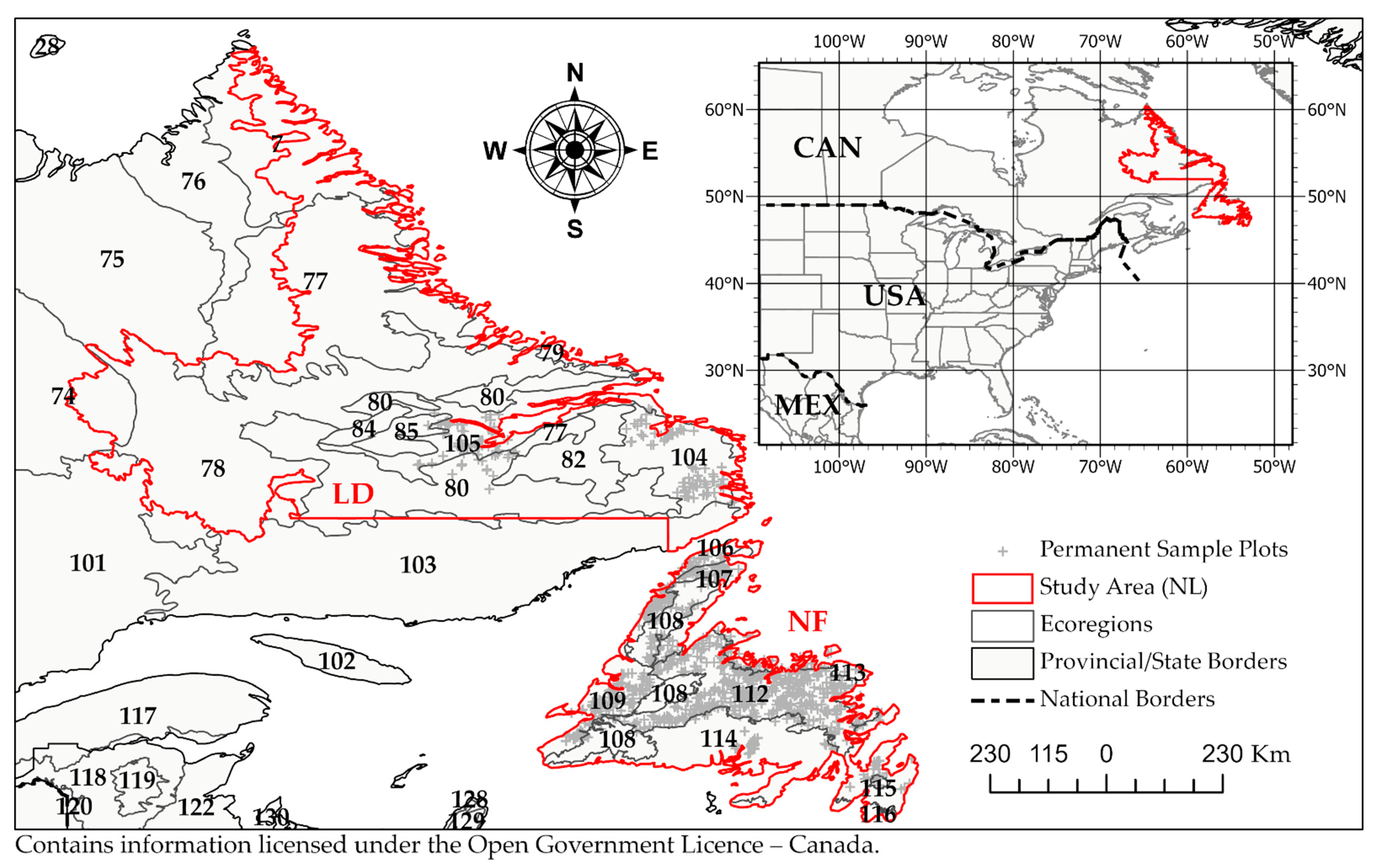
2.1. Study Area

The study area for this paper was the province of Newfoundland and Labrador (Figure 1). NL falls both within Canada’s boreal shield and taiga shield ecozones and contains 23 ecoregion growing environments per the Canadian Ecological Land Classification Framework [55] (

Table 1. Land area and plot inventory statistics by ecoregion in Newfoundland and Labrador.

Ecoregion		Land Area		Permanent Sample Plot Inventory
ID	Common Name	A	AP	n	PP
7	Torngat Mountains	18,391	4.58	0	0
75	Ungava Bay Basin	1018	0.25	0	0
77	Kingarutuk-Fraser River	50,612	12.59	2	0.17
74	New Quebec Central Plateau	8091	2.01	0	0
78	Smallwood Reservoir-Michikamau	77,380	19.25	0	0
79	Coastal Barrens	13,690	3.41	3	0.26
80	Mecatina River	52,960	13.18	16	1.4
82	Eagle Plateau	13,320	3.31	0	0
84	Harp Lake	3122	0.78	0	0
85	Nipishish Lake	5134	1.28	1	0.09
101	Central Laurentians	1959	0.49	0	0
103	Mecatina Plateau	6722	1.67	1	0.09
104	Paradise River	19,400	4.83	83	7.24
105	Lake Melville	18,011	4.48	62	5.41
106	Strait of Belle Isle	2485	0.62	21	1.83
107	Northern Peninsula	8118	2.02	128	11.17
108	Long Range Mountains	16,115	4.01	40	3.49
109	Southwestern Newfoundland	10,691	2.66	149	13
112	Central Newfoundland	30,217	7.52	499	43.54
113	Northeastern Newfoundland	5712	1.42	55	4.8
114	Maritime Barrens	36,224	9.01	78	6.81
115	Avalon Forest	493	0.12	8	0.7
116	South Avalon-Burin Oceanic Barrens	2078	0.52	0	0
		401,941	-	1146	-

A: ecoregion land area (km²); AP: proportion of the total provincial land area within the ecoregion (%); n: number of permanent sample plots representing the ecoregion; P_P: the proportion of the total permanent sample plot inventory representing the ecoregion (%).

). Newfoundland (NF) is an 11 million ha island of which 45% is boreal forest [58]. Climate information available through Environment and Climate Change Canada [59] indicates precipitation rates are relatively even across NF, with some seasonal variation (750 to 2000 mm year⁻¹). Coastal locations across the province experience slightly greater precipitation and more mild temperatures as opposed to inland geographies due to the moderating effect of the sea. In northern locations across NF, annual snowfall can exceed 300 cm and constitutes half of the annual precipitation. In the milder southeast, snowfall accounts for only 10% of total annual precipitation. January mean daily temperatures in NF range from −4 to −10 °C, whereas July mean daily temperature is approximately 16 °C.

Continental Labrador (LD) contains roughly 18 million ha of boreal forest, making up approximately 60% of the region’s total land area [60]. The cumulative annual precipitation range tends to be less than that observed in NF (725 to 1250 mm year⁻¹). As with NF, coastal locations in LD are subject to the moderating influence of the sea. January mean temperature ranges between −16 and −25 °C across LD, whereas July mean daily temperature ranges between 6 and 13 °C. A 50-year summary of historical climate (i.e., precipitation and growing degree days) is provided in Table S1.

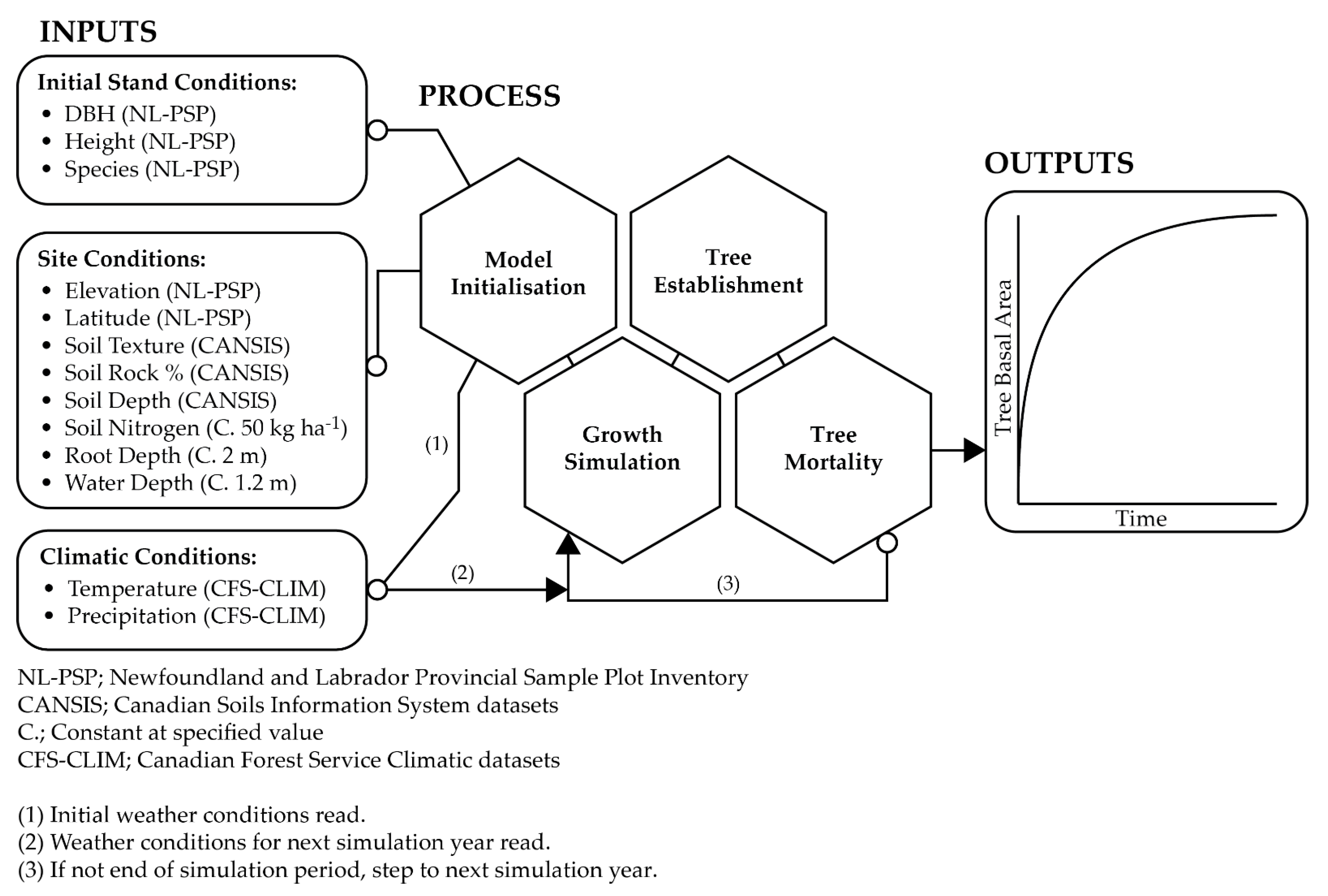
2.2. Model Description

We used the JABOWA-3 forest gap model to prepare projections of forest growth under RCP 2.6, 4.5, and 8.5. An RCP refers to a greenhouse gas trajectory that has been adopted by the Intergovernmental Panel on Climate Change [1]. Each RCP entails a different global climate outcome, which may be realized subject to realized emissions over coming years. The RCPs are uniquely defined by total radiative forcing, which is a cumulative measure of human emissions of greenhouse gases from all sources expressed in W/m² (i.e., 2.6, 4.5, and 8.5 W/m², respectively, in this study) [5].

JABOWA uses a static, small plot setup (i.e., 0.01 ha) to model forest growth and succession on an annual timestep. JABOWA is underpinned by a number of key assumptions through which the model formalizes the complex processes associated with tree growth, establishment, and mortality through a relatively simplistic functional design [38]: (i) the forest is abstracted as a composite of many small patches of land, where each patch can have a different age and successional stage; (ii) patches are horizontally homogenous, i.e., a tree’s position within a patch is not considered or significant; (iii) the leaves of each tree are located in a thin layer at the top of the stem, otherwise relieving the need to calculate shading and thus competitive effects associated with tree position; and (iv) successional processes can be described for each of those patches separately, i.e., there are no interactions between patches, and the forest is a mosaic of independent patches. In JABOWA, diameter growth is modelled through a deterministic process based on maximum potential behaviour, which is reduced by factors including limiting light, soil fertility, soil moisture, and temperature effects [38,41].

JABOWA’s growth model is accompanied by two sub-models for tree mortality and establishment. Through the tree establishment sub-model, saplings are added only where biotic (light) and abiotic (temperature and moisture) conditions are satisfied: (i) Light availability at the forest floor meets a species-specific threshold (i.e., leaf area index (LAI)), (ii) the annual sum of actual evapotranspiration (AET) must lie above a species-specific threshold value, and (iii) the annual sum of degree days is within a parameter-specified range tolerated by the species (i.e., DD_Min and DD_Max) [38,41]. Species-specific degree-day ranges were modified in this study to improve model usability in the northerly reaches of the study area. The methods and rationale for this adjustment to species growing degree-day ranges are described in the Supplementary Materials. JABOWA’s mortality sub-model is a stochastic process involving two components: (i) “intrinsic” or “background” mortality, which permits only 2% of trees from reaching the parameter-specified maximum tree age (i.e., A_Max)—this mortality function is species-specific and constant across a tree’s life—and (ii) a “competitive” or “stress-related” mortality function that acts when a tree’s diameter growth increment is less than 0.01 cm for any given year. JABOWA’s competitive mortality function is based on the premise that a tree has a 1% chance of surviving 10 consecutive years if stressed. As soon as there is no stress, the stress-related mortality ceases to be relevant. Hence, it is assumed that there are no lags between the occurrence of stress and the associated mortality, and that stress tolerance is not species-specific. A simplified and conceptual flow of JABOWA’s processes, inputs, and outputs is provided in Figure 2. A comprehensive review of the function of the JABOWA family is provided in Botkin [41]. Bugmann [38] provides an excellent synopsis of the history and generalized processes that underpin the JABOWA family of models.

2.3. Model Inputs

Each of JABOWA’s inputs can be classified into one of three types: initial stand conditions, site conditions, or climatic conditions [39] (Figure 2).

2.3.1. Initial Stand Conditions

In this study, initial stand conditions were based on permanent sample plot (PSP) data provided by the NL Department of Fisheries, Forestry and Agriculture. The database includes a network of approximately 1150 plots, 630,000 individual tree diameter breast height (DBH) measurements, and 430,000 growth ($\Delta$DBH) measurements, spanning a period from 1985–2017. Nine of the province’s boreal species were included in the scope of this study (

Table 2. Species code, common name, binomial (i.e., scientific) name, and authority.

Code	Common	Binomial
BF	Balsam fir	Abies balsamea (L.) Mill
BS	Black spruce	Picea mariana (Mill.) Britton et al.
WS	White spruce	Picea glauca (Moench) Voss
WB	White birch	Betula papyrifera Marshall
YB	Yellow birch	Betula alleghaniensisi Britt.
RM	Red maple	Acer rubrum L.
WP	White pine	Pinus strobus L.
TA	Trembling aspen	Populus tremuloides Michx.
TL	Tamarack (Eastern larch)	Larix laricina (Du Roi) K. Koch

). The nine species selected account for the vast majority of the province’s tree species (

Table 3. Species occurrence as a proportion of all tree observations recorded within an ecoregion (ID) between 2000 and 2017.

ID	Species Occurrence as % of Total Observations (2000–2017)
	BF	BS	RM	TL	TA	WB	WP	WS	YB	Other
77	79.89	0.00	0.00	0.00	0.00	6.90	0.00	13.22	0.00	0.00
79	35.88	58.56	0.00	4.12	0.00	1.24	0.00	0.21	0.00	0.00
80	30.43	52.56	0.85	2.62	1.99	9.90	0.00	0.42	0.00	1.23
85	15.63	84.38	0.00	0.00	0.00	0.00	0.00	0.00	0.00	0.00
103	73.17	26.83	0.00	0.00	0.00	0.00	0.00	0.00	0.00	0.00
104	39.99	46.56	0.00	0.14	1.36	10.62	0.00	1.15	0.00	0.17
105	35.50	55.91	0.30	0.27	0.66	4.53	0.00	0.68	0.00	2.15
106	86.64	4.51	0.00	0.20	0.00	1.86	0.00	6.77	0.00	0.02
107	81.88	8.46	0.01	0.14	0.00	6.81	0.00	2.16	0.16	0.37
108	80.35	10.52	0.55	0.00	0.00	5.40	0.00	3.02	0.10	0.06
109	77.58	13.58	0.27	0.19	0.00	5.50	0.02	2.30	0.24	0.33
112	33.50	57.99	0.35	0.65	0.46	4.58	0.06	1.65	0.00	0.75
113	20.97	75.73	0.12	0.50	0.13	2.32	0.00	0.14	0.00	0.09
114	57.20	37.02	0.00	2.37	0.36	2.04	0.00	0.11	0.33	0.57
115	87.42	0.00	0.00	0.00	0.00	12.31	0.00	0.00	0.26	0.00
Total	50.20	41.23	0.25	0.56	0.34	5.02	0.03	1.70	0.08	0.58

ID: ecoregion ID, see Table 1.

) and all commercially significant species [58].

Plots where disturbance regimes (i.e., moose browsing, fire, pests, and windthrow) were documented to have influenced tree growth were removed from the pool of plots used in this analysis. Although JABOWA does have subroutines for certain disturbances (e.g., windthrow and logging), other important disturbances (e.g., forest pests, moose browsing, fire) cannot be simulated through the unmodified program. In removing disturbance plots, 259 plots and approximately 600 plot measurements were removed from the study. Deadwood and/or snag tree observations were also removed from the database as the competitive influence of snags and standing deadwood are not considered in JABOWA.

Plots range in size from 0.002 to 0.1 ha, including an array of intermediate sizes. The size of PSPs is not fixed in NL’s inventory and commonly increases as a plot matures over remeasurement occasions and stem density declines. A remeasurement occasion refers to any subsequent PSP measurement following the initial plot establishment measurement. Plot remeasurement does not occur on an annual interval in NL’s PSP inventory program, but rather at periods typically ranging from 3 to 7 years. Differing plot areas impact JABOWA’s density and light-level subroutines, which assume a 0.01 ha plot area. Through the data formatting process, all PSP measurements were scaled to a standard 0.01 ha; this process is described in the Supplementary Materials section.

2.3.2. Site Conditions

Soil texture, stoniness, and depth were obtained for each plot in NL’s inventory from the Soil Landscapes of Canada (SLC) datasets, sourced from the National Soil Database [61]. Elevation and latitude for each plot were recorded through NL’s PSP inventory program. Soil nitrogen and depth-to-water information is not available at the site level in NL, and so soil fertility (i.e., nitrogen) and depth-to-water parameters were held constant at 50 kg ha⁻¹ and 1.2 m, respectively. These assumptions do influence JABOWA’s growth predictions, as they impact subroutines which measure the impact of soil nutrient and chemical cycling, as well as functions for water balance and moisture conditions, respectively [41], so these fixed rates are a limitation of this study.

2.3.3. Climatic Conditions

Climatic conditions for the model calibration phase of the work were based on estimates of historical monthly cumulative precipitation, monthly mean daily minimum, and maximum temperature timeseries constructed for every PSP from 1985 to 2010 (Table S2). The datasets were generated using thin-plate smoothing splines, as implemented in ANUSPLIN [62]. ANUSPLIN is a multidimensional nonparametric surface fitting method that offers the capacity to generate estimates of dependent variables at any location where the independent variables are known—in this case longitude, latitude, and elevation [63,64]. The historical monthly models have 95% confidence limits of approximately ± 1.1 °C for maximum temperature, ± 1.3 °C for minimum temperature, and ± 10–40% for monthly precipitation [63,64].

For the simulation phase of this study, monthly mean minimum and maximum temperatures and monthly cumulative precipitation projections were obtained from 2020 to 2100 under RCPs 2.6 (Table S3), 4.5 (Table S4), and 8.5 (Table S5). The scenarios were downscaled from predictions of the CanESM2 global climate model as developed by Chylek et al. [65] and implemented by McKenney et al. [63,64] through their ANUSPLIN generation of digital climate surfaces.

2.4. Model Calibration

Prior to model validation, an initial calibration was performed using a stratified random selection of approximately 40% of the plots contained within each ecoregion included in the analysis. Stratifying the random selection of calibration plots by ecoregion ensured the full spectrum of growing conditions affecting tree growth in the PSP inventory would be captured in those plots used to calibrate JABOWA-3. Plots located in ecoregions 75, 79, 85, 103, and 115 were altogether removed from the study at this stage as the number of plots (i.e., < 10 plots) representing those ecoregions was not sufficient to conduct a valuable calibration or validation exercise (Table 1).

Calibration was performed in iterations. JABOWA parameters were manually adjusted between iterations to optimize the fit between model-generated (i.e., simulated) basal area (BA, m² ha⁻¹) and observed BA at remeasurement occasions. Simulated and observed BA pairs were further stratified by species to inform the manual adjustment of model parameters for specific species. JABOWA’s parameters were manually adjusted within limits considered to be ecologically and physiologically reasonable. A manual approach to calibration is standard in studies that attempt to apply process-based modelling software [14,39,66,67,68,69]. The final parameter values used in this study are provided in Table S1.

Each iteration of JABOWA involved systematically initializing the model for each PSP used in calibration by establishing the initial model conditions as those observed in the corresponding plot establishment record (see Figure 2). Historical weather records were used in JABOWA to simulate tree growth for the period between plot establishment and the most recent plot remeasurement. Calibration outputs were taken as the average of 50 simulations to lessen the effect of model stochasticity brought on by model functions of mortality.

In both the model calibration and validation phases, species entry into a simulation for reasons of establishment was restricted to those observed within the plot at any plot measurement in the PSP program; this limitation is further explored in the discussion. This was done to limit erroneous species “migration” into the plot, but also restricted feasible species migration into the plot where a species may be present in the greater area, but not within the plot measured. In the absence of data describing species composition in the vicinity of the plot, we were unable to adjust entry permissions to allow any species establishment beyond those observed within the plot.

2.5. Model Validation

In this study, we use the term “validation” to refer to an empirical comparison of model-generated (i.e., simulated) plot BA values against corresponding plot BA observations. Model validation utilized the JABOWA parameter settings identified through calibration and was based on pairs of simulated and observed BA not used in the model calibration phase—that is, approximately 60% of the plots in the PSP inventory. As with calibration, validation stratified pairs of simulated and observed BA by species. Two approaches, statistical analysis and model-efficiency testing [39], were used to evaluate the predictive performance of the model both in terms of overall fit and fit at specific remeasurement occasions. The latter evaluation at specific remeasurement occasions allowed for analysis of the model performance at varying temporal points from model initialization. Put simply, analysis at specific remeasurement occasions allowed us to evaluate whether the performance of the model degraded or otherwise changed at observations temporally further from model initialization.

A common method used in model validation is to evaluate a simple linear regression between field observed, Y, and simulated, X, values, where Y_s = b₀ + b₁X_s [39,70]. In this study, Y is the observed BA (m² ha⁻¹) for species s, and X is the simulated BA for the same species. Variables b₀ and b₁ are the intercept and slope of regression, respectively. In an ideal model, the linear fit is b₁ ~ 1 through the origin (b₀ = 0) [71]. The adequacy of the model can therefore be evaluated by determining whether b₀ = 0 and b₁ = 1 with separate t-tests [71], assuming a linear relationship between observed and predicted values. Similarly, a simultaneous F-test can be used to evaluate the regression Y_s = b₀ + b₁X_s by testing whether b₀ = 0 and b₁ = 1 simultaneously. Both tests were used in this study to determine the statistical significance of slope for unity and intercept for zero [71,72]. In addition to the separate t-tests and simultaneous F-tests, model bias (Equation (1)), model efficiency (ME, Equation (2)), and root mean square error (RMSE, Equation (3)) were also determined to garner further insight into the performance of the identified JABOWA-3 settings in modelling growth in NL:

$$Bias=\frac{{{\displaystyle \sum }}_{i=1}^n\left(BA{o}_i-BA{p}_i\right)}{n}$$

(1)

$$ME=1-\frac{{{\displaystyle \sum }}_{i=1}^n{\left(BA{o}_i-BA{p}_i\right)}^2}{{{\displaystyle \sum }}_{i=1}^n{\left(BA{o}_i-{\overline{BAo}}_i\right)}^2}$$

(2)

$$RMSE=\sqrt{\frac{{{\displaystyle \sum }}_{i=1}^n{\left(BA{o}_{i,j}-BA{p}_{i,j}\right)}^2}{n}}$$

(3)

where $BA{o}_{ij}$ and $BA{p}_{ij}$ are the observed and modelled BA of species j at time interval $i$ in a particular PSP, and ${\overline{BAo}}_i$ is the mean of the observed value of all observations in the validation dataset for all time periods. Where RMSE, bias, and ME were calculated for specific remeasurement occasions, Equations (1)–(3) were applied against a subset of the validation dataset, where $BA{o}_{ij}$, $BA{p}_{ij}$, ${\overline{BAo}}_i$, and n refer only to observations corresponding to a specific selection of remeasurement observation(s). Yellow birch (n = 13) and white pine (n = 12) did not occur frequently enough in the validation dataset to be subsetted by remeasurement occasion (Table 2); the validation exercise was only conducted against full validation dataset for these two species. Combined, yellow birch and white pine constituted 0.1% of the full PSP inventory (Table 3).

The ME coefficient was originally developed as the model efficiency coefficient (NSE) by Nash and Sutcliffe [73] to assess the predictive power of hydrological models. The coefficient is an index with a range from −∞ to 1.0, where ME = 1.0, the model fits the observations perfectly, and where ME = 0.0 the model is no better than a simple average of all the data [22,39,74]. In application, efficiency values between 0.5 and 0.65 are suggested to represent a model of sufficient quality [75,76].

2.6. Growth Scenarios

Following validation, JABOWA-3 was used to simulate a series of four forest growth scenarios: a “reference” scenario, and three scenarios under RCP 2.6, 4.5, and 8.5—“low”, “moderate,” and “high” concentration pathways, respectively. Each scenario spanned an 80-year period from 2020 to 2100. Growth scenario simulation included every plot in the study program (i.e., the combined calibration and validation datasets). As with model calibration and validation, initial stand conditions for each plot in the growth scenario phase of this study were set as those recorded through plot establishment records. Differing from calibration and validation processes, however, through growth scenario simulation establishment records were initialized in 2019, regardless of the actual time when the establishment measurement took place. Such an approach facilitated the use of plot establishment records as the initial conditions in growth scenarios, which were otherwise measured at some point between 1985 and 2017. This approach also best facilitated forest growth comparison both between the varied RCP scenarios and under the reference scenario, as all scenarios were based on the same initial set of initial forest conditions.

Under the reference scenario, the historical climate dataset (Table S1), having occurred between 1960 and 2015, was applied to the growth scenarios simulated between 2020 and 2100. By default, JABOWA uses weather records in a repeated manner, where the simulation horizon exceeds the weather records provided.

2.7. Growth Modifiers

Growth modifiers (GM) were prepared as the difference between simulated growth under the reference scenario and simulated growth under the RCP 2.6, 4.5, and 8.5 scenarios:

$$C{k}_{c,j,i}=\frac{BA{c}_{j,i}}{BA{a}_{j,i}}$$

(4)

where $C{k}_{c,i,t}$ are species-specific GM accounting for the effect of climate change on tree growth, $BA{c}_{i,t}$ is the predicted average BA under a specific climate change scenario (i.e., RCP 2.6, 4.5, 8.5) c, and $BAa$ is the average BA under the reference scenario. The GM can then be applied to an empirical growth projection:

$$BA{m}_{c,i,t}=BA{e}_{i,t}·C{k}_{c,i,t}$$

(5)

where $BA{e}_{i,t}$ is the projected basal area using an empirical model, and $BA{m}_{c,i,t}$ is the modified basal area forecast under climate change scenario c.

3. Results

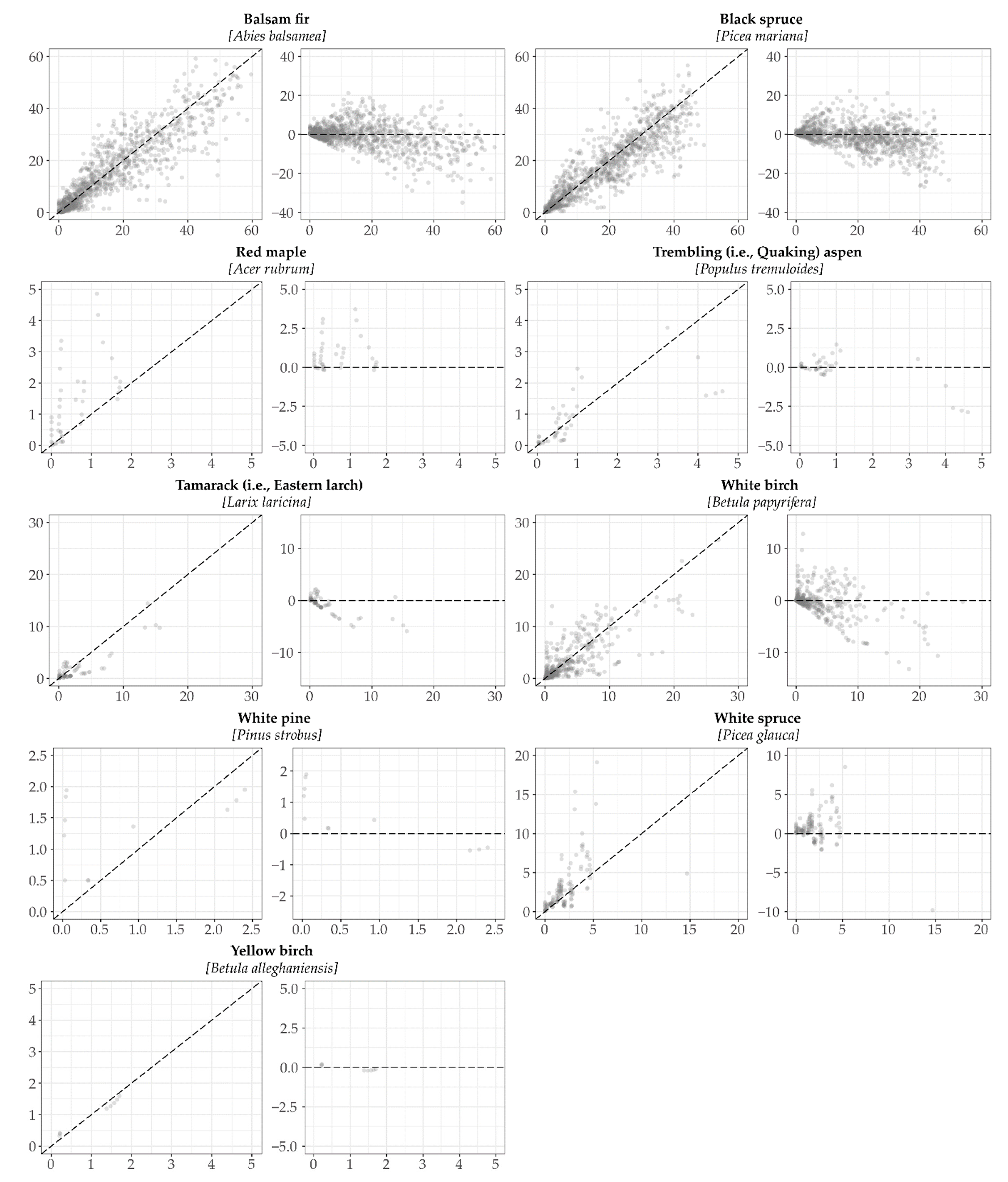
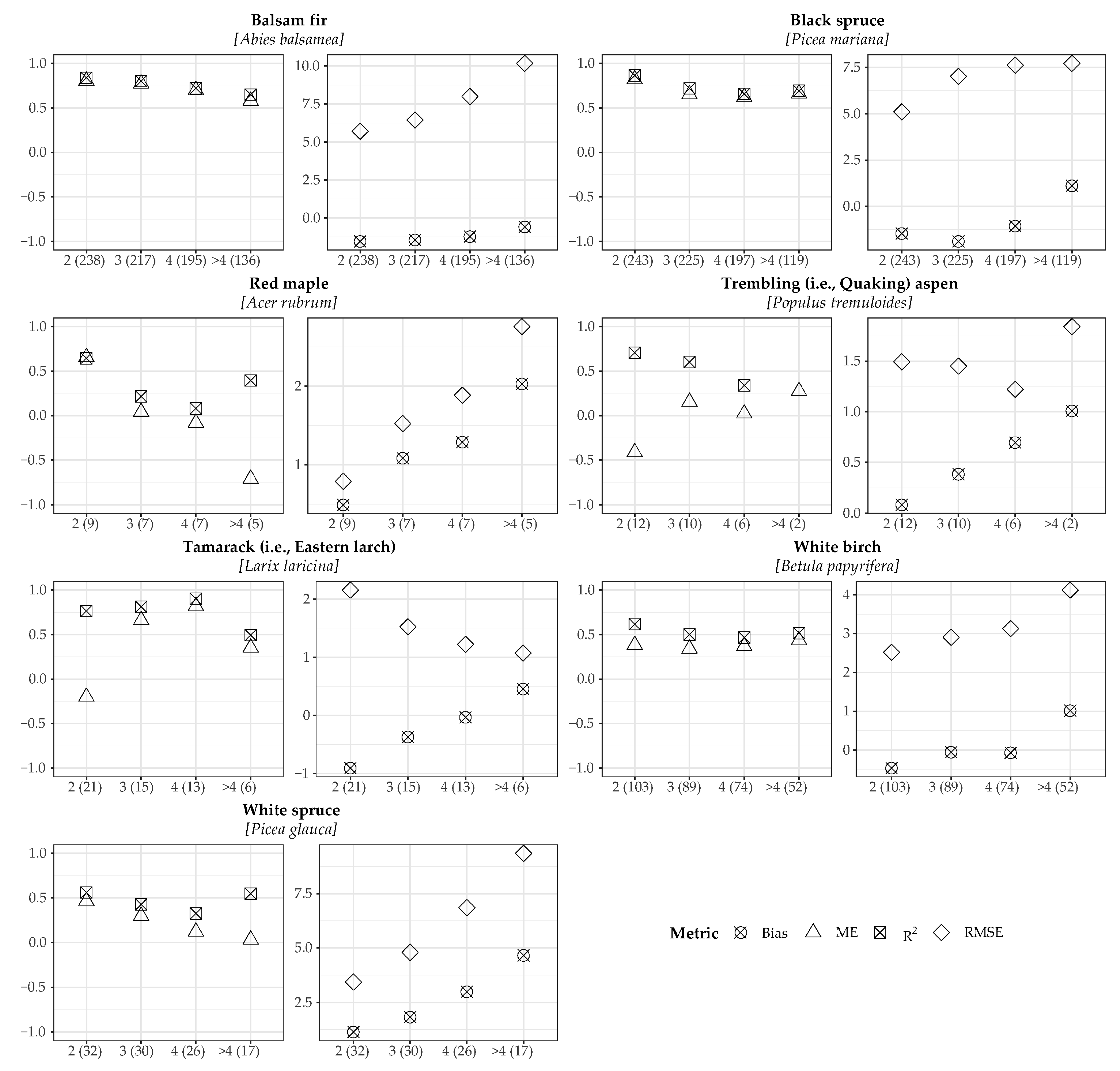
3.1. Model Validation

Separate t- and F-tests produced high p-values for each of the nine boreal species included in this study, demonstrating that in general, estimated slope and intercept were not significantly different from unity and zero (

Table 4. Overall evaluation of JABOWA-3 by species.

Species	n	Bias	R2	RMSE	ME	Regression Coefficients Y = (b0+b1X)		Slope (b1) = 1 and Intercept (b0) = 0 α = 0.05
								Separate t-Test (df = n-2)		Simultaneous F-Test (df = 2 and n-2)
								t	p	F	p
WB	437	−0.15	0.61	2.84	0.51	b0	0.80	5.09	< 0.001	57.14	< 0.001
						b1	0.71	26.14	< 0.001
BF	1057	−1.10	0.79	6.81	0.76	b0	2.23	7.83	< 0.001	93.05	< 0.001
						b1	0.83	63.80	< 0.001
TL	77	−0.52	0.78	1.73	0.39	b0	0.08	0.53	0.60	52.83	< 0.001
						b1	0.65	16.40	< 0.001
TA	46	0.03	0.62	2.76	−0.29	b0	0.42	3.83	< 0.001	95.29	< 0.001
						b1	0.40	8.67	< 0.001
BS	1063	−0.95	0.78	6.13	0.75	b0	2.19	6.99	< 0.001	95.03	< 0.001
						b1	0.83	61.36	< 0.001
WS	142	1.86	0.24	5.29	0.24	b0	0.72	1.33	0.19	10.79	< 0.001
						b1	1.40	6.82	< 0.001
RM	41	0.88	0.31	1.52	0.14	b0	0.66	2.99	0.005	12.87	< 0.001
						b1	1.22	4.36	< 0.001
YB	8	0.07	0.99	0.33	0.89	b0	0.21	5.16	0.002	30.38	< 0.001
						b1	0.76	23.29	< 0.001
WP	13	0.19	0.26	0.78	−0.41	b0	1.12	5.81	< 0.001	19.30	< 0.001
						b1	0.29	2.29	0.04
	2884	−0.67	0.83	5.79	0.80	b0	1.45	10.29	< 0.001	223.91	< 0.001
						b1	0.85	118.10	< 0.001

n: number of simulated and observed pairs; ME: model efficiency; RMSE: root mean square error.

). As notable exceptions to this, the intercepts of both tamarack and white spruce observed vs. modelled data showed significant deviation from both unity and zero (p < 0.05). Balsam fir (Abies balsamea (L.) Mill), black spruce (Picea mariana (Mill.) Britton et al.), and white birch (Picea glauca (Moench) Voss) were all found to have R² > 0.6, ME > 0.5, and RMSE < 7.0 m² ha⁻¹ (Table 4), indicating that the simulated BA generally agreed with the observation. For balsam fir, black spruce, and white birch (Figure 3), plotted simulated vs. observed data followed the diagonal whereas residual plots were generally dispersed along the horizontal; both distributions further suggested agreement between the simulated and observed BA. A heteroscedastic distribution was, however, present in the balsam fir, black spruce, and white birch plots (Figure 3), indicating that absolute model error for these species increased with BA. Observed plot BA values ranged up to 60 m² ha⁻¹ for black spruce and balsam fir, and up to 30 m² ha⁻¹ for white birch. Most observed BA values were below 30 m² ha⁻¹ for each of the three species. Residuals generally ranged between –20 and 20 m² ha⁻¹ for balsam fir and black spruce, and from –10 to 10 m² ha⁻¹ for white birch.

The validation process was not satisfactory for less abundant species, including tamarack (Larix laricina (Du Roi) K. Koch), trembling aspen (Populus tremuloides Michx.), white spruce (Picea glauca (Moench) Voss), red maple (Acer rubrum L. 1753), yellow birch (Betula alleghaniensisi Britt.), and white pine (Pinus strobus L.). For these species, R² ranged from 0.244 (white spruce) to 0.779 (tamarack) and ME from −0.413 (white pine) to 0.887 (yellow birch) (Table 4). Save for the exception of yellow birch (R² = 0.99, ME = 0.89, n = 8; Table 4), R² and ME would not both meet the threshold of 0.5 used as an indicator of good simulation agreement. The simulated vs. observed and residuals plots for these same species did not generally follow any pattern, leaving us to conclude that the JABOWA simulations in this study struggled to accurately forecast growth for these species. As an exception, white spruce did exhibit a simulated vs. observed plot that approximated a diagonal relationship, and residuals that approximated a horizontal (though highly heteroscedastic) distribution (Figure 3). Nonetheless, R² for white spruce was low compared to other conifers modelled (R² = 0.24), as was ME (ME = 0.24, Table 4). Analysis of these same metrics at specified remeasurement occasions (Figure 4) identified that agreement between simulated and observed white spruce BA tended to erode as the model progressed.

We evaluated model performance at specific points in time by extracting subsets of predicted and observed data pairs corresponding to specific observation re-measurements from the validation dataset and calculated RMSE, Bias, R², and ME indicators using the subsets (Figure 4). With respect to balsam fir and black spruce, we found ME and R² to be above 0.5 across all remeasurement occasions, confirming that agreement between simulated and observed black spruce and balsam fir BA values does not significantly degrade at remeasurement occasions further from the plot establishment measurement. With respect to white birch, ME and R² were found to both be between 0.4 and 0.5, depending on the remeasurement year, indicating reasonable agreement between simulated and observed BA values, but not as strong as those documented for balsam fir or black spruce. In general, the plots presented in Figure 4 offered further confirmation that simulated BA for red maple, trembling aspen, white spruce, and tamarack did not generally agree with observed BA values. Although modelled values were satisfactory for some of these species at specific remeasurement occasions (e.g., red maple at remeasurement 2 and tamarack at remeasurements 3 and 4; Figure 4), model settings yielded conflicting results at other intervals. Bias and RMSE for red maple, trembling aspen, white spruce, and tamarack seemed to identify that simulated values for these species became increasingly conservative (i.e., less simulated growth than observed) at years further from initialization. We observed time (i.e., remeasurement occasion) to influence BA simulation bias and RMSE in all species considered (Figure 4). The nature of RMSE and bias relationships to remeasurement occasion was species dependent. With respect to balsam fir, bias and RMSE appeared to compound while moving away from model initialization, increasing with remeasurement occasion. This characterization was not shared with observed bias and RMSE for black spruce, which appeared to better approximate a logarithmic relationship between RMSE and remeasurement occasion. Bias and RMSE for white birch BA were also found to approximate an exponential curve, as with balsam fir, albeit at a shallower slope (Figure 4).

3.2. Growth Scenarios and Modifiers

Simulated growth by model scenario, species, and ecoregion is provided in Table S6. GM are provided at an annual timestep by climate scenario, species, and ecoregion in Table S7. Figure 5 and Figure 6 are graphical representations of those large tabular datasets. The relative abundances of all nine tree species were generally held constant over the 80-year simulation period under each of the four growth scenarios (Figure 5). We observed average plot basal area to range between 20 m² ha⁻¹ and 30 m² ha⁻¹ across the province through to the 80-year simulation period (Figure 5). This range was consistent across the reference scenario and those associated with RCPs 2.6, 4.5, and 8.5. Accordingly, we found deviations in simulated BA growth to be relatively modest when comparing simulated BA under RCPs 2.6, 4.5, and 8.5 to simulated BA under the reference scenario (< 50% departure from the reference scenario, as measured at 2100; Figure 6). There were, however, instances where this generalization did not hold true: (i) In the Strait of Belle Isle ecoregion, a departure of > 100% for black spruce was observed under the RCP 2.6 and 4.5 scenarios and ± 50% under the RCP 8.5 scenario; (ii) in the Mecatina River, Paradise River, and Lake Melville ecoregions, a departure of > 100% for white birch BA was observed under the RCP 2.6 scenario; (iii) and in the Lake Melville ecoregion, this same departure of > 100% for white birch BA was also present in the RCP 4.5 and 8.5 model scenarios (Figure 6).

We observed increased conifer productivity (i.e., black spruce, balsam fir) in northerly ecoregions when comparing BA growth under the RCP 2.6, 4.5, and 8.5 scenarios to the reference scenario (i.e., the Mecatina River, Paradise River, Lake Melville, Strait of Belle Isle, and Northern Peninsula ecoregions). In these regions, black spruce BA was found to be 10 and 30% greater by 2100 under RCPs 2.6, 4.5 and 8.5 as compared to the reference scenario (Figure 6). Similarly, balsam fir BA in LD was observed to be between 10 and 80% greater by 2100 under RCPs 2.6, 4.5 and 8.5 as compared to the reference scenario (Figure 6). Conversely, in the study area’s more southerly ecoregions (i.e., the Long Range Mountains, Southwestern Newfoundland, Central Newfoundland, Northeastern Newfoundland, and the Maritime Barrens), conifer productivity was found to either be maintained or otherwise be slightly reduced through as simulated at 2100. In the Long Range Mountains and Maritime Barrens ecoregions, simulations for black spruce and balsam fir BA were found to be between 0 and 40% less and 5% more to 40% less by 2100, respectively. These departures in productivity were moderated to some extent by model scenario (Figure 6).

At the study area’s more southerly latitudes, growth simulations under the RCP high concentration pathway typically resulted in a notably lower average plot BA versus that simulated under the moderate, low, and reference scenarios; see, for instance, the simulations for the Central Newfoundland, Maritime Barrens, and Northeastern Newfoundland ecoregions. In contrast, in NL’s northmost PSPs, average plot BA under the high, moderate, and low concentration pathway each was higher than that of the reference scenario; see, for example, simulations for the Mecatina River, Paradise River, and Lake Melville ecoregions (Figure 5). We frequently observed average plot BA to increase over the short to mid term (5–40 years, Figure 5). This initial increase in mean productivity would generally be between 5 and 10 m² ha⁻¹ as compared to the reference scenario. The rate at which average BA would reach a maximum varied mostly by ecoregion rather than by model scenario. Some plots realized maximum average BA within the first 10 years of the simulation (e.g., the Paradise River and Long Range Mountains ecoregions), whereas in others maximum average BA would not be realized for 30 or more years (e.g., the Central and Northeastern Newfoundland ecoregions, Figure 5). After reaching maximum average plot BA, average plot BA tended to either plateau at the end of the simulation or otherwise face a very slight decline (Figure 5).

A comparison of scenario outcomes then informed the preparation of GM (Table S7). Although GM were calculated for each of the nine species in this study, only those for black spruce, balsam fir, and white birch were backed by good model validation results (Table 4, Figure 3 and Figure 4). GM for black spruce ranged from 0.6 to 2.3, generally falling between 0.8 and 1.3. For balsam fir, GM ranged from 0.7 to 1.8, generally falling between 0.9 and 1.2. For white birch, GM ranged from 0.2 to 3.0, generally falling between 0.9 and 1.4 (Table S7). GM can theoretically be used to adjust empirical G&Y predictions, making them more robust for use under scenarios of climate change.

4. Discussion

An evaluation of model predictive performance is an important step prior to application. Simulated BA largely agreed with observed BA for the three most abundant species components of NL boreal forests (Table 3); balsam fir, black spruce, and white birch were all found to have R² > 0.6, ME > 0.5, and RMSE < 7.0 m² ha⁻¹ (Table 4). Considering the entire PSP dataset (n = 2,884), validation held an R² and ME of 0.83 and 0.80, respectively (Table 4). Although there have been no applications of a PBM in Canada’s northeastern Atlantic region that predate this work, there have been recent applications of PBM in the New England–Acadian transitional forests of Canada’s maritime provinces that have had similar success in modelling forest dynamics through PBM methods [14,39].

In another application of JABOWA-3 in Nova Scotia, Canada, Ashraf et al. [39] reported an R² of 0.97 and ME 0.96. Our study is structurally different than most other applications of PBM, including that completed by Ashraf et al., in that it applies JABOWA-3 to each qualifying plot in the full inventory program, rather than use representative plots as the basis of inference on the full plot dataset. Ashraf et al. [39] used a representative plot study structure, which facilitated the plot-level adjustments to model settings necessary to attain excellent agreement between simulated and observed BA not only of boreal conifers, including black spruce and balsam fir, but also other important New England–Acadian species as well, such as red maple, red spruce (Picea rubens Sarg.), eastern hemlock (Tsuga canadensis (L.) Carrière), and red oak (Quercus rubra L.). The trade-off in achieving good model agreement in a select number of plots is that the identified model settings are less certain when applied elsewhere in the study area. In contrast, our study was only able to attain good model evaluation results for black spruce, balsam fir, and white birch. However, we had a high degree of confidence that the identified model settings were appropriate for use within the large study area. Furthermore, black spruce, balsam fir, and white birch constitute more than 96% of NL’s tree inventory and include the species of the greatest commercial significance to the province [58]. Although improved evaluation results for the less abundant species of NL’s PSP inventory would be ideal, it is likely that the relative scarcity of these species (i.e., red maple, trembling aspen, tamarack, and white spruce) and the consequent low number of observed and simulated pairs inhibited the identification of satisfactory model settings in this study. Ashraf et al. [39] also observed that the JABOWA-3 mortality subroutine appeared to underpredict mortality in some instances, particularly with respect to mature overstory. Our work corroborates these findings; we observed that maximum individual tree DBH and average individual tree DBH increased with stand age (Table S6). Two factors likely contributed to this anomaly: (i) the absence of large forest renewal events through stand-level disturbance, and (ii) JABOWA-3′s parameter values being based on tree dimensions observed in the transitional New England–Acadian forests of New Hampshire [41], rather than those observed in NL. Concerning the latter factor, we could have adjusted JABOWA-3′s H_Max, A_Max, and D_Max parameters (Table S1) to reflect conditions in NL, however, we observed that doing so resulted in undesirable effects on the rate of growth in simulations as JABOWA’s growth functions. Furthermore, the two factors are related, as it is difficult to decouple the role of disturbance on the maximum dimensions observed through NL’s PSP inventory.

The results from our simulations only partially agree with our hypothesis. Provincial-scale warming to 2100 [77] will generally have a modest, but positive effect on the northerly black spruce and balsam fir forests of NL. This characterization is not reflective of simulation outcomes for the province’s southernmost forests (Figure 6), where conifer BA under RCPs 2.6, 4.5, and 8.5 was often found to either be generally consistent with, or slightly less than, BAs observed under the reference scenario (Figure 6). This observation corroborates a growing library of empirical studies that propose that increased conifer productivity at northerly latitudes may well be one “positive” socio-economic externality attributed to contemporary climate projections [15,16,17]. Other recent applications of PBM in Atlantic Canada, such as that completed by Taylor et al. [14], have found that the transitional forests of the New England–Acadian forest region may begin to lose its boreal character as cornerstone boreal species fail to regenerate and survive beginning at the mid-point of the century under certain RCPs (i.e., RCP 8.5). It is crucial to recognize that the compositional shifts in transition zone forest makeup are generally thought to be driven by changes in competitive interactions attributed to climate change, rather than due to climate change itself [13,14,78,79]. Our study did identify that boreal forest growth may slow and even decline at lower latitudes within the study area under high RCPs, such as RCP 8.5, but found no evidence that the dominant conifer species of NL’s forests will be replaced within the 80-year horizon used in this study (i.e., 2100). The caveat to the foregoing is that species entry into a plot was restricted through model settings, and so our observation is based only on the lack of dramatic changes in current species proportions of plots through the simulation period. The markedly lower species diversity of the northeastern boreal forest as compared to that of the New England–Acadian forest region insulates NL’s cool-adapted boreal conifer forests from the excessive proliferation of warm adapted temperate tree species.

This study also sought to prepare an approach to modelling G&Y that would remain robust under the changing climate of the future. To achieve this, we derived a series of time-dependent forest GM that can be readily applied to empirical G&Y models through a simple multiplicative process [56,57]. The approach adjusts empirical projections based on the simulated influence of changing future climate as modelled through PBM methods. The GM method preserves the strengths of the empirical G&Y model, including the relatively simple parameterizations, high predictive accuracy, and alignment with operational demands, while leveraging the strengths of the PBM method in order to generate more reliable growth predictions for use under scenarios of climate change. The GM prepared (Table S7), although subject to a series of important caveats and limitations through this study, offer a viable theoretical approach through which forest response to changing climate can be readily integrated with sustainable forest management strategies.

4.1. Implications on Sustainable Forest Management

Our study indicates that under local warming trends anticipated for NL under scenarios 2.6, 4.5, and 8.5, the boreal forests of NL will experience an uneven response in terms of growth and establishment. Whereas in the northernmost reaches of the province conifer productivity may generally be bolstered, conifer productivity in the southern locations may only be maintained, and in some instances even erode under anticipated warming (Figure 6). In NL, conifers constituted 98% of the annual allowable cut between 2011 and 2015, with 88% of conifer volume originating from NF and 12% from LD [58]. Black spruce and balsam fir together make up an overwhelming majority of the province’s lumber and pulpwood harvest volume. Only 11% of the annual allowable cut between 2011 and 2015 originated from the Strait of Belle Isle and Northern Peninsula ecoregions. These are the only ecoregions in NF where black spruce and balsam fir productivity was identified to increase in response to the projected warming trends. In general, gains in productivity in the northern locations of NF and LD outpace productivity losses at the province’s southerly isotherms (Figure 6). Local warming trends may well warrant further consideration of NL’s allocation of annual allowable cut volumes considering the identified mixed regional productivity impacts on boreal conifers. Our results support a growing body of evidence that identifies that global taiga and boreal forests along northern isotherms may experience increased productivity under future climate projections, where growing degree days (GDD) have traditionally served as a limiting factor to tree growth.

4.2. Caveats and Limitations

Although our methods are themselves a source of certain limitations, other limitations were inherited through JABOWA-3, as well as the various datasets used in determining input parameters. Perhaps most significantly, we were not able to confirm the suitability of model settings for tamarack, trembling aspen, white spruce, red maple, yellow birch, and white pine that supported acceptable validation results (Table 4). This is most likely due to the relative scarcity of these species compared to the dominant species components of NL’s PSP inventory, i.e., balsam fir, black spruce, and white birch (Table 3). These species generally have a low number of occurrences in PSPs in NL’s inventory program; combined, tamarack, trembling aspen, white spruce, red maple, yellow birch, and white pine constitute less than 3% of the total PSP inventory. When attempting to evaluate model performance at the plot level using plots that typically only contain a small number of instances of certain species, real individual tree status effects (e.g., suppression, mortality, pests, etc.) not adequately reflected in the more generalized PBM can generate large discrepancies in simulated plot-level BA where individual specimens constitute a large portion of plot BA for a species in a plot. Put simply, it may be a matter of representing the population and mean successional processes generally well, but perhaps not the growth of the individual. Nevertheless, we included tamarack, trembling aspen, white spruce, red maple, yellow birch, and white pine in our simulations to preserve their competitive influence on those species in which agreement between observed and simulated BA values was observed. Simulations and GM for tamarack, trembling aspen, white spruce, red maple, yellow birch, and white pine are included in Table S7 for reference but are not supported by fair model validation results, as GM for black spruce, balsam fir, and white birch are.

None of the models or GM prepared herein account for the influence of most forest disturbances. Studies have found that the influence of these important regenerative events can be expected to evolve under a changing future climate [80,81]. JABOWA-3 is not structured to adequately consider a full spectrum of forest disturbance events, nor changes in the frequency and intensity of such events over time with changing climate. Consequently, the projections put forward in this study are insulated from stand-level events that serve to “reset” forest composition and structure to a point of lesser maturity. This is a particularly important consideration in certain regions of NL where windthrow and fire regimes are common drivers of forest successional processes [82,83,84].

We simulated BA growth based on individual plots across the province of NL. Through our simulations JABOWA’s species entry parameter was restricted to those species observed within the plot through any measurement taken as part of NL’s PSP inventory. This restriction was imposed to moderate the potential for erroneous species “migration” into plots through the simulation period. This same position also worked to artificially constrain species migration into a plot in instances where a species may exist in the local area, but outside the plot being simulated. Further related to the JABOWA parameterizations employed, we used the forest conditions present in PSP establishment records as the prevailing conditions in the base year for growth simulation (i.e., 2020). Plot establishment conditions were used as base-year conditions regardless of when establishment records were logged. Given that plot establishment records vary in their date of measure, the growth predictions herein are not to be considered as an explicit model of the composition and structure of the province’s forested areas over the study horizon. Rather, our scenarios offer a point of comparison from which the growth influence of RCPs 2.6, 4.5, and 8.5 can be compared both amongst themselves and against an additional scenario that utilizes a historical climate dataset. The GM prepared through our work are an operationalization of the comparative analysis facilitated.

Although we observed that the model settings remained robust at points as temporally distant as five plot remeasurements (± 15–25 years) from plot establishment record and model initialization, we were unable to confirm the model performance over longer time frames. The 80-year simulation horizon employed in this study is a considerably longer period than that used to evaluate model performance. Some uncertainty originates from using the model beyond the horizon used to evaluate, particularly with regard to deviations in simulated BA values from those observed, as discussed. This is particularly notable in this study with respect to balsam fir, where RMSE and bias seemed to compound over the simulation horizon. This is despite R² and ME remaining above the 0.5 threshold for the species, which was used in this study as an indicator of good model performance. Of course, the precise simulation of real-world BA is inherently challenging over long simulation horizons, as the influence of stochastic forest events is commonly a major contributor in forest growth trends over long growing horizons [41].

Further limitations and uncertainty were inherited by the SLC and climatic datasets used in setting key parameters in JABOWA-3. The former dataset, the SLC, is a series of GIS layers that contain the major characteristics of soil and land at a national scale, with national coverage (1:1,000,000) [61]. As such, the SLC tends to generalize soil conditions across large geographic space and can misrepresent the specific soil conditions at a site level. Despite this, no alternative soil information with full coverage of the study area was available to us for this work. With respect to the climate datasets used, limited station coverage in NL does influence the ability of the ANUSLPLIN-generated models to capture spatial and temporal variation in precipitation estimates at the site level. In both cases, the use of a large PSP dataset in both model evaluation and projection exercises reduces the influence of any one plot on the overall average where the conditions in the plot may be misrepresented at the site level through the datasets supplied.

Also related to model inputs, this study was inhibited by a lack of available fine-scale depth-to-water data. As such, JABOWA’s depth-to-water parameter (DT) was set to a uniform 1.25 m for every plot in the PSP inventory. For most boreal species in NL, this parameterization presents neither a constraint, nor optimal conditions for growth [41]. The implicit assumption in the use of such a constant is that growing environment moisture is not, at present, a limiting condition to growth in most of the plots in NL’s PSP inventory [17]. Further still, there would be an equal number of plots where surplus moisture is a limiting factor and moisture deficit is a limiting factor in a true census PSP inventory. Of course, we have no way of confirming either of the above, and so there is significant uncertainty in our simulations where the water balance is concerned and its relationship to actual conditions within a plot. This uncertainty becomes somewhat diluted where we use scales as coarse as ecoregions to evaluate the regional influence of climatic changes, rather than do so at the plot level, but uncertainty from a lack of real DT information nevertheless remains and would certainly bolster this analysis if made available. We are not the only study to cite data limitations as a key pitfall in applying PBM [14,56]. As discussed, demanding parameterizations have served as a key barrier to operational use of PBM for some time. As a consequence, there is developing scientific interest in supporting research that seeks to improve the quality environmental data used to parameterize PBM, which would strengthen the ability of researchers to quantify and understand the reliability of PBM simulations [85].

5. Conclusions

The study was carried out to determine the suitability of using a PBM as part of a method for attaining robust predictions of forest G&Y under scenarios of climate change in NL, Canada. Our model evaluation found JABOWA-3 to be suited for modelling the growth of black spruce, balsam fir, and white birch within the province, but less appropriate for modelling the growth of the less abundant components of NL’s forest make-up, such as red maple, white spruce, white pine, yellow birch, trembling aspen, and tamarack. A simulation of BA to 2100 under representative concentration pathways (RCPs) 2.6, 4.5, and 8.5 indicates that changing climate might stand to bolster BA within the study area that are cooler under present-day conditions (such as Labrador). Conversely, productivity was found to be at best maintained, and even decline, in the warmer present-day growing sites within the province. These projections then informed GM values, which can be used to adjust projections from empirical models for improved reliability under future climate regimes.

References

1. Intergovernmental Panel on Climate Change. Climate Change 2013: The Physical Science Basis; Climate Change 2013; Intergovernmental Panel on Climate Change: New York, NY, USA, 2014; p. 1552. [Google Scholar]
2. Morison, J.I.L.; Morecroft, M.D. (Eds.) Plant Growth and Climate Change; Blackwell Publishing Ltd.: Oxford, UK, 2006; ISBN 9780470988695. [Google Scholar]
3. Babst, F.; Bouriaud, O.; Poulter, B.; Trouet, V.; Girardin, M.P.; Frank, D.C. Twentieth Century Redistribution in Climatic Drivers of Global Tree Growth. Sci. Adv. 2019, 5, eaat4313. [Google Scholar] [CrossRef] [PubMed] [Green Version]
4. Oboite, F.O.; Comeau, P.G. Competition and Climate Influence Growth of Black Spruce in Western Boreal Forests. For. Ecol. Manag. 2019, 443, 84–94. [Google Scholar] [CrossRef]
5. van Vuuren, D.P.; Edmonds, J.; Kainuma, M.; Riahi, K.; Thomson, A.; Hibbard, K.; Hurtt, G.C.; Kram, T.; Krey, V.; Lamarque, J.-F.; et al. The Representative Concentration Pathways: An Overview. Clim. Chang. 2011, 109, 5–31. [Google Scholar] [CrossRef]
6. Charney, N.D.; Babst, F.; Poulter, B.; Record, S.; Trouet, V.M.; Frank, D.; Enquist, B.J.; Evans, M.E.K. Observed Forest Sensitivity to Climate Implies Large Changes in 21st Century North American Forest Growth. Ecol. Lett. 2016, 19, 1119–1128. [Google Scholar] [CrossRef] [PubMed]
7. Tremblay, G.D.; Boudreau, S. Black Spruce Regeneration at the Treeline Ecotone: Synergistic Impacts of Climate Change and Caribou Activity. Can. J. For. Res. 2011, 41, 460–468. [Google Scholar] [CrossRef]
8. Michaelian, M.; Hogg, E.H.; Hall, R.J.; Arsenault, E. Massive Mortality of Aspen Following Severe Drought along the Southern Edge of the Canadian Boreal Forest. Glob. Chang. Biol. 2011, 17, 2084–2094. [Google Scholar] [CrossRef] [Green Version]
9. Hogg, E.H.; Michaelian, M.; Hook, T.I.; Undershultz, M.E. Recent Climatic Drying Leads to Age-Independent Growth Reductions of White Spruce Stands in Western Canada. Glob. Chang. Biol. 2017, 23, 5297–5308. [Google Scholar] [CrossRef]
10. Esquivel-Muelbert, A.; Baker, T.R.; Dexter, K.G.; Lewis, S.L.; Brienen, R.J.W.; Feldpausch, T.R.; Lloyd, J.; Monteagudo-Mendoza, A.; Arroyo, L.; Álvarez-Dávila, E.; et al. Compositional Response of Amazon Forests to Climate Change. Glob. Chang. Biol. 2019, 25, 39–56. [Google Scholar] [CrossRef] [Green Version]
11. Klos, R.J.; Wang, G.G.; Bauerle, W.L.; Rieck, J.R. Drought Impact on Forest Growth and Mortality in the Southeast USA: An Analysis Using Forest Health and Monitoring Data. Ecol. Appl. 2009, 19, 699–708. [Google Scholar] [CrossRef]
12. Liu, H.; Park Williams, A.; Allen, C.D.; Guo, D.; Wu, X.; Anenkhonov, O.A.; Liang, E.; Sandanov, D.V.; Yin, Y.; Qi, Z.; et al. Rapid Warming Accelerates Tree Growth Decline in Semi-Arid Forests of Inner Asia. Glob. Chang. Biol. 2013, 19, 2500–2510. [Google Scholar] [CrossRef]
13. Boulanger, Y.; Taylor, A.R.; Price, D.T.; Cyr, D.; McGarrigle, E.; Rammer, W.; Sainte-Marie, G.; Beaudoin, A.; Guindon, L.; Mansuy, N. Climate Change Impacts on Forest Landscapes along the Canadian Southern Boreal Forest Transition Zone. Landsc. Ecol. 2017, 32, 1415–1431. [Google Scholar] [CrossRef]
14. Taylor, A.R.; Boulanger, Y.; Price, D.T.; Cyr, D.; McGarrigle, E.; Rammer, W.; Kershaw, J.A. Rapid 21st Century Climate Change Projected to Shift Composition and Growth of Canada’s Acadian Forest Region. For. Ecol. Manag. 2017, 405, 284–294. [Google Scholar] [CrossRef]
15. Berner, L.T.; Beck, P.S.A.; Bunn, A.G.; Goetz, S.J. Plant Response to Climate Change along the Forest-Tundra Ecotone in Northeastern Siberia. Glob. Change Biol. 2013, 3449–3462. [Google Scholar] [CrossRef]
16. Price, D.T.; Alfaro, R.I.; Brown, K.J.; Flannigan, M.D.; Fleming, R.A.; Hogg, E.H.; Girardin, M.P.; Lakusta, T.; Johnston, M.; McKenney, D.W.; et al. Anticipating the Consequences of Climate Change for Canada’s Boreal Forest Ecosystems. Environ. Rev. 2013, 21, 322–365. [Google Scholar] [CrossRef]
17. Searls, T.; Zhu, X.; McKenney, D.W.; Mazumder, R.; Steenberg, J.; Yan, G.; Meng, F.-R. Assessing the Influence of Climate on the Growth Rate of Boreal Tree Species in Northeastern Canada through Long Term Permanent Sample Plot Datasets. Can. J. For. Res. 2020. [Google Scholar] [CrossRef]
18. Noseworthy, J.; Beckley, T.M. Borealization of the New England—Acadian Forest: A Review of the Evidence. Environ. Rev. 2020, 28, 284–293. [Google Scholar] [CrossRef]
19. Bouchard, M.; Pothier, D.; Gauthier, S. Fire Return Intervals and Tree Species Succession in the North Shore Region of Eastern Quebec. Can. J. For. Res. 2008, 38, 1621–1633. [Google Scholar] [CrossRef]
20. Régnière, J.; St-Amant, R.; Duval, P. Predicting Insect Distributions under Climate Change from Physiological Responses: Spruce Budworm as an Example. Biol. Invasions 2012, 14, 1571–1586. [Google Scholar] [CrossRef]
21. Boulanger, Y.; Gauthier, S.; Burton, P.J. A Refinement of Models Projecting Future Canadian Fire Regimes Using Homogeneous Fire Regime Zones. Can. J. For. Res. 2014, 44, 365–376. [Google Scholar] [CrossRef]
22. Vanclay, J.K.; Skovsgaard, J.P. Evaluating Forest Growth Models. Ecol. Model. 1997, 98, 1–12. [Google Scholar] [CrossRef] [Green Version]
23. Porté, A.; Bartelink, H.H. Modelling Mixed Forest Growth: A Review of Models for Forest Management. Ecol. Model. 2002, 150, 141–188. [Google Scholar] [CrossRef]
24. Korzukhin, M.D.; Ter-Mikaelian, M.T.; Wagner, R.G. Process versus Empirical Models: Which Approach for Forest Ecosystem Management? Can. J. For. Res. 1996, 26, 879–887. [Google Scholar] [CrossRef]
25. Paulsen, J.C. Kurze Praktische Anleitung zun Forstwesen. Verfasst von Einem Forstmanne; Verfasst Von Einem Forstmanne: Detmold, Germany, 1795. [Google Scholar]
26. Von Cotta, H. Hülfstafeln für Forstwirte und Forsttaxatoren; Arnoldische Buchhandlung: Dresden, Germany, 1821. [Google Scholar]
27. Sullivan, A.D.; Clutter, J.L. A Simultaneous Growth and Yield Model for Loblolly Pine. For. Sci. 1972, 18, 76–86. [Google Scholar] [CrossRef]
28. Subedi, N.; Sharma, M. Individual-Tree Diameter Growth Models for Black Spruce and Jack Pine Plantations in Northern Ontario. For. Ecol. Manag. 2011, 261, 2140–2148. [Google Scholar] [CrossRef]
29. Battaglia, M.; Sands, P.J. Process-Based Forest Productivity Models and Their Application in Forest Management. For. Ecol. Manag. 1998, 102, 13–32. [Google Scholar] [CrossRef]
30. Johnsen, K.; Samuelson, L.; Teskey, R.; McNulty, S.; Fox, T. Process Models as Tools in Forestry Research and Management. For. Sci. 2001, 47, 2–8. [Google Scholar]
31. Vanclay, J.K. Modelling Forest Growth and Yield: Applications to Mixed Tropical Forests; CAB International: Wallingford, UK, 1994; ISBN 9780851989136. [Google Scholar]
32. Yaussy, D.A. Comparison of an Empirical Forest Growth and Yield Simulator and a Forest Gap Simulator Using Actual 30-Year Growth from Two Even-Aged Forests in Kentucky. For. Ecol. Manag. 2000, 126, 385–398. [Google Scholar] [CrossRef]
33. Kimmins, J.P. Forest Ecology: A Foundation for Sustainable Forest Management and Environmental Ethics in Forestry, 3rd ed.; Prentice Hall: Upper Saddle River, NJ, USA, 2004; ISBN 9780130662583. [Google Scholar]
34. Gustafson, E.J. When Relationships Estimated in the Past Cannot Be Used to Predict the Future: Using Mechanistic Models to Predict Landscape Ecological Dynamics in a Changing World. Landsc. Ecol. 2013, 28, 1429–1437. [Google Scholar] [CrossRef]
35. Kimmins, J.P. Modelling the Sustainability of Forest Production and Yield for a Changing and Uncertain Future. For. Chron. 1990, 66, 271–280. [Google Scholar] [CrossRef] [Green Version]
36. Monserud, R.A. Evaluating Forest Models in a Sustainable Forest Management Context. For. Biometry Model. Inf. Sci. 2003, 1, 35–47. [Google Scholar]
37. Pinjuv, G.; Mason, E.G.; Watt, M. Quantitative Validation and Comparison of a Range of Forest Growth Model Types. For. Ecol. Manag. 2006, 236, 37–46. [Google Scholar] [CrossRef]
38. Bugmann, H. A Review of Forest Gap Models. Clim. Chang. 2001, 51, 259–305. [Google Scholar] [CrossRef]
39. Ashraf, M.I.; Bourque, C.P.-A.; MacLean, D.A.; Erdle, T.; Meng, F.-R. Using JABOWA-3 for Forest Growth and Yield Predictions under Diverse Forest Conditions of Nova Scotia, Canada. For. Chron. 2012, 88, 708–721. [Google Scholar] [CrossRef]
40. Landsberg, J. Modelling Forest Ecosystems: State of the Art, Challenges, and Future Directions. Can. J. For. Res. 2003, 33, 385–397. [Google Scholar] [CrossRef]
41. Botkin, D.B. Forest Dynamics: An Ecological Model; Oxford University Press: Oxford, UK, 1993; ISBN 9780195065558. [Google Scholar]
42. Botkin, D.B.; Janak, J.F.; Wallis, J.R. Some Ecological Consequences of a Computer Model of Forest Growth. J. Ecol. 1972, 60, 849. [Google Scholar] [CrossRef] [Green Version]
43. Bossel, H.; Krieger, H. Simulation Model of Natural Tropical Forest Dynamics. Ecol. Model. 1991, 59, 37–71. [Google Scholar] [CrossRef]
44. Larocque, G.R.; Archambault, L.; Delisle, C. Development of the Gap Model ZELIG-CFS to Predict the Dynamics of North American Mixed Forest Types with Complex Structures. Ecol. Model. 2011, 222, 2570–2583. [Google Scholar] [CrossRef]
45. Shugart, H.H.; West, D.C. Development of an Appalachian Deciduous Forest Succession Model and Its Application to Assessment of the Impact of the Chestnut Blight. J. Environ. Manag. 1977, 5, 161–179. [Google Scholar]
46. Shugart, H.H. A Theory of Forest Dynamics: The Ecological Implications of Forest Succession Models; Blackburn Press: Caldwell, NJ, USA, 2003; ISBN 9781930665750. [Google Scholar]
47. Aber, J.D.; Botkin, D.B.; Melillo, J.M. Predicting the Effects of Different Harvesting Regimes on Forest Floor Dynamics in Northern Hardwoods. Can. J. For. Res. 1978, 8, 306–315. [Google Scholar] [CrossRef]
48. Urban, D.L.; Bonan, G.B.; Smith, T.M.; Shugart, H.H. Spatial Applications of Gap Models. For. Ecol. Manag. 1991, 42, 95–110. [Google Scholar] [CrossRef]
49. Lexer, M.J.; Hönninger, K. A Modified 3D-Patch Model for Spatially Explicit Simulation of Vegetation Composition in Heterogeneous Landscapes. For. Ecol. Manag. 2001, 144, 43–65. [Google Scholar] [CrossRef]
50. Bugmann, H.K.M. A Simplified Forest Model to Study Species Composition Along Climate Gradients. Ecology 1996, 77, 2055–2074. [Google Scholar] [CrossRef]
51. Pacala, S.W.; Canham, C.D.; Saponara, J.; Silander, J.A.; Kobe, R.K.; Ribbens, E. Forest Models Defined by Field Measurements: Estimation, Error Analysis and Dynamics. Ecol. Monogr. 1996, 66, 1–43. [Google Scholar] [CrossRef]
52. Köhler, P.; Ditzer, T.; Huth, A. Concepts for the Aggregation of Tropical Tree Species into Functional Types and the Application to Sabah’s Lowland Rain Forests. J. Trop. Ecol. 2000, 16, 591–602. [Google Scholar] [CrossRef]
53. Köhler, P.; Huth, A. The Effects of Tree Species Grouping in Tropical Rainforest Modelling: Simulations with the Individual-Based Model Formind. Ecol. Model. 1998, 109, 301–321. [Google Scholar] [CrossRef] [Green Version]
54. Ngugi, M.R.; Botkin, D.B. Validation of a Multispecies Forest Dynamics Model Using 50-Year Growth from Eucalyptus Forests in Eastern Australia. Ecol. Model. 2011, 222, 3261–3270. [Google Scholar] [CrossRef]
55. Ecological Stratification Working Group (Canada). A National Ecological Framework for Canada; The Group: Ottawa, ON, Canada, 1996; ISBN 9780662241072. [Google Scholar]
56. Ashraf, M.I. A Framework for Predicting Forest Growth and Yield under Projected Climate Change. Ph.D. Thesis, University of New Brunswick, Fredericton, NB, Canada, 2013. [Google Scholar]
57. Miao, Z.; Li, C. Predicting Tree Growth Dynamics of Boreal Forest in Response to Climate Change. In Landscape Ecology in Forest Management and Conservation; Li, C., Lafortezza, R., Chen, J., Eds.; Springer: Berlin/Heidelberg, Germany, 2011; pp. 176–205. ISBN 9783642127533. [Google Scholar]
58. Government of Newfoundland and Labrador, Department of Natural Resources. Growing Our Renewable and Sustainable Forest Economy: Provincial Sustainable Forest Management Strategy (2014–2024); Government of Newfoundland and Labrador, Department of Natural Resources: St. John’s, NL, Canada, 2014; p. 66.
59. Environment and Climate Change Canada. Canadian Climate Normals & Averages; Environment and Climate Change Canada: Ottawa, ON, Canada, 2019. [Google Scholar]
60. Environment and Climate Change Canada. Forest Land by Province and Territory; Environment and Climate Change Canada: Ottawa, ON, Canada, 2011. [Google Scholar]
61. Agriculture and Agri-Food Canada. National Soil DataBase; Agriculture and Agri-Food Canada, Government of Canada: Ottawa, ON, Canada, 2020.
62. Hutchinson, M.F. Interpolating Mean Rainfall Using Thin Plate Smoothing Splines. Int. J. Geogr. Inf. Syst. 1995, 9, 385–403. [Google Scholar] [CrossRef]
63. McKenney, D.W.; Hutchinson, M.F.; Papadopol, P.; Lawrence, K.; Pedlar, J.; Campbell, K.; Milewska, E.; Hopkinson, R.F.; Price, D.; Owen, T. Customized Spatial Climate Models for North America. Bull. Am. Meteorol. Soc. 2011, 92, 1611–1622. [Google Scholar] [CrossRef]
64. McKenney, D.; Pedlar, J.; Hutchinson, M.; Papadopol, P.; Lawrence, K.; Campbell, K.; Milewska, E.; Hopkinson, R.F.; Price, D. Spatial Climate Models for Canada’s Forestry Community. For. Chron. 2013, 89, 659–663. [Google Scholar] [CrossRef] [Green Version]
65. Chylek, P.; Li, J.; Dubey, M.K.; Wang, M.; Lesins, G. Observed and Model Simulated 20th Century Arctic Temperature Variability: Canadian Earth System Model CanESM2. Atmos. Chem. Phys. Discuss. 2011, 11, 22893–22907. [Google Scholar] [CrossRef]
66. Chiesi, M.; Maselli, F.; Moriondo, M.; Fibbi, L.; Bindi, M.; Running, S.W. Application of BIOME-BGC to Simulate Mediterranean Forest Processes. Ecol. Model. 2007, 206, 179–190. [Google Scholar] [CrossRef]
67. Lindner, M.; Sievänen, R.; Pretzsch, H. Improving the Simulation of Stand Structure in a Forest Gap Model. For. Ecol. Manag. 1997, 95, 183–195. [Google Scholar] [CrossRef]
68. Pabst, R.J.; Goslin, M.N.; Garman, S.L.; Spies, T.A. Calibrating and Testing a Gap Model for Simulating Forest Management in the Oregon Coast Range. For. Ecol. Manag. 2008, 256, 958–972. [Google Scholar] [CrossRef]
69. Risch, A.C.; Heiri, C.; Bugmann, H. Simulating Structural Forest Patterns with a Forest Gap Model: A Model Evaluation. Ecol. Model. 2005, 181, 161–172. [Google Scholar] [CrossRef]
70. Huang, S.; Price, D.; Morgan, D.; Titus, S. Validation of Ecoregion-Based Taper Equations for White Spruce in Alberta. For. Chron. 1999, 75, 281–292. [Google Scholar] [CrossRef]
71. Yang, Y.; Monserud, R.A.; Huang, S. An Evaluation of Diagnostic Tests and Their Roles in Validating Forest Biometric Models. Can. J. Forest Res. 2004, 34, 11. [Google Scholar] [CrossRef]
72. Moore, D.S.; Notz, W.; Fligner, M.A. The Basic Practice of Statistics, 6th ed.; W.H. Freeman: New York, NY, USA, 2013; ISBN 9781464102547. [Google Scholar]
73. Nash, J.E.; Sutcliffe, J.V. River Flow Forecasting through Conceptual Models Part I—A Discussion of Principles. J. Hydrol. 1970, 10, 282–290. [Google Scholar] [CrossRef]
74. Soares, P.; Tomé, M.; Skovsgaard, J.P.; Vanclay, J.K. Evaluating a Growth Model for Forest Management Using Continuous Forest Inventory Data. For. Ecol. Manag. 1995, 71, 251–265. [Google Scholar] [CrossRef]
75. Moriasi, D.N.; Arnold, J.G.; Van Liew, M.W.; Bingner, R.L.; Harmel, R.D.; Veith, T.L. Model Evaluation Guidelines for Systematic Quantification of Accuracy in Watershed Simulations. Trans. ASABE 2007, 50, 885–900. [Google Scholar] [CrossRef]
76. Ritter, A.; Muñoz-Carpena, R. Performance Evaluation of Hydrological Models: Statistical Significance for Reducing Subjectivity in Goodness-of-Fit Assessments. J. Hydrol. 2013, 480, 33–45. [Google Scholar] [CrossRef]
77. Finnis, J.; Daraio, J. Projected Impacts of Climate Change for the Province of Newfoundland & Labrador: 2018 Update; Memorial University of Newfoundland: St. John’s, NL, Canada, 2018; p. 134. [Google Scholar]
78. Rogers, B.M.; Jantz, P.; Goetz, S.J. Vulnerability of Eastern US Tree Species to Climate Change. Glob. Chang. Biol. 2017, 23, 3302–3320. [Google Scholar] [CrossRef]
79. Steenberg, J.W.N.; Duinker, P.N.; Bush, P.G. Exploring Adaptation to Climate Change in the Forests of Central Nova Scotia, Canada. For. Ecol. Manag. 2011, 262, 2316–2327. [Google Scholar] [CrossRef]
80. Burlando, P.; Rosso, R. Extreme Storm Rainfall and Climatic Change. Atmos. Res. 1991, 27, 169–189. [Google Scholar] [CrossRef]
81. Dash, C.B.; Fraterrigo, J.M.; Hu, F.S. Land Cover Influences Boreal-Forest Fire Responses to Climate Change: Geospatial Analysis of Historical Records from Alaska. Landsc. Ecol. 2016, 31, 1781–1793. [Google Scholar] [CrossRef]
82. Robertson, A. The Centroid of Tree Crowns as an Indicator of Abiotic Processes in a Balsam Fir Wave Forest. Can. J. For. Res. 1987, 17, 746–755. [Google Scholar]
83. Ruel, J.-C. Understanding Windthrow: Silvicultural Implications. For. Chron. 1995, 71, 434–445. [Google Scholar]
84. Arsenault, A.; LeBlanc, R.; Earle, E.; Brooks, D.; Clarke, B.; Lavigne, D.; Royer, L. Unravelling the Past to Manage Newfoundland’s Forests for the Future. For. Chron. 2016, 92, 487–502. [Google Scholar]
85. Urban, M.C.; Bocedi, G.; Hendry, A.P.; Mihoub, J.-B.; Peer, G.; Singer, A.; Bridle, J.R.; Crozier, L.G.; De Meester, L.; Godsoe, W.; et al. Improving the Forecast for Biodiversity under Climate Change. Science 2016, 353, aad8466. [Google Scholar] [CrossRef] [Green Version]
Figure 1. Permanent sample plot distribution and ecoregion map of Newfoundland and Labrador. The numbers are associated with the individual ecoregions identified in Table 1.
Forests 12 00248 g001
Figure 2. A conceptual summary of JABOWA’s parameterizations, processes, and outputs, as well as the datasets or constants used as inputs in this study.
Forests 12 00248 g002
Figure 3. Simulated basal area (X, m2 ha−1) and observed BA (Y, m2 ha−1) plots (left), as well as simulated BA (X, m2 ha−1) and residual (Y, m2 ha−1) plots (right) by species.
Forests 12 00248 g003
Figure 4. Model efficiency (ME) and R2 metrics by plot remeasurement occasion (left) as well as bias (m2 ha−1) and root mean square error (RMSE, m2 ha−1) metrics (right) by plot remeasurement occasion. Metrics are measured along the y-axis, whereas plot remeasurement is along the x-axis; the number of observations associated with each remeasurement is denoted by brackets ().
Forests 12 00248 g004
Figure 5. Simulated average individual plot basal area (m2 ha−1) disambiguated by species between 2020 and 2100 by ecoregion and climate scenario. Maximum and minimum individual plot basal area by scenario and ecoregion is also plotted.
Forests 12 00248 g005
Figure 6. Percentage deviation in simulated growth from the reference scenario by species, climate projection, and ecoregion.
Forests 12 00248 g006