Abstract
Percent tree cover maps derived from Landsat imagery provide a useful data source for monitoring changes in tree cover over time. Urban trees are a special group of trees outside forests (TOFs) and occur often as solitary trees, in roadside alleys and in small groups, exhibiting a wide range of crown shapes. Framed by house walls and with impervious surfaces as background and in the immediate neighborhood, they are difficult to assess from Landsat imagery with a 30 m pixel size. In fact, global maps based on Landsat partly failed to detect a considerable portion of urban trees. This study presents a neural network approach applied to the urban trees in the metropolitan area of Bengaluru, India, resulting in a new map of estimated tree cover (MAE = 13.04%); this approach has the potential to also detect smaller trees within cities. Our model was trained with ground truth data from WorldView-3 very high resolution imagery, which allows to assess tree cover per pixel from 0% to 100%. The results of this study may be used to improve the accuracy of Landsat-based time series of tree cover in urban environments.
1. Introduction
Trees, especially when of larger dimensions, are considered key ecological elements in many non-forest land use systems, including urban areas [1,2]. There they serve manifold functions including ecological, environmental and economic. Urban trees are one type of what has been termed “trees outside forests” (TOF; e.g., [3,4,5]), a concept that is currently receiving increasing attention when devising measures for mitigation of climate change, for conservation of biodiversity and for Forest Landscape Restoration (FLR) [6]. India is among the earliest countries, if not the first, that has integrated the assessment of TOF and urban trees into its National Forest Monitoring Program [7].
The assessment of tree cover, including the generation of maps [8], yields basic information that supports the monitoring of ecosystem services provided by trees [9]. In this context, remote sensing data are essential components of large area tree monitoring systems, as they can provide observations on a spatially continuous scale over larger areas. Rapid developments in computational performance have made it possible to observe tree cover and forest changes [10,11], even at a global level. When it comes to mapping individual TOF, however, these global maps are often not sufficient, as the highly fragmented pattern of tree cover is hardly captured, and this holds also for urban trees which mainly come in three basic spatial patterns: (1) solitary and scattered trees (for example, in home gardens), (2) groups of trees (patches) that may form closed canopies (for example, in parks) and (3) alleys along streets whose crowns, depending on the development stage, can cover large areas.
In and around emerging megacities, rapid changes in land-use and land-cover are taking place, which result in a highly diverse and fragmented landscape [12] and a dramatic change in tree density and tree crown cover [13]. With a comparatively coarse resolution of 30 m, Landsat images over such urban landscapes contain a high proportion of mixed pixels so that, per pixel, the spectral response of more than one class is recorded, and this reduces the chance of accurate classification in the resulting maps. To nevertheless produce satisfactorily accurate results, additional pre-processing steps are required on a sub-pixel level, such as spectral unmixing techniques (e.g., spectral mixture analysis) [14,15,16] or the use of soft or fuzzy classification methods [17]. Although classification accuracy increased in the studies utilizing sub-pixel analyses, there is still a gap when it comes to the detection of isolated, individual tree crowns below the Landsat pixel size of 900 m2. Then, the spectral response of tree crowns is mixed with the spectral response of various other objects and usually spread over more than one pixel. This is of particular relevance in complex urban environments, where objects with very different reflection characteristics are close together. The very frequent occurrence of mixed pixels makes classification and mapping of scattered urban tree covers challenging. Systematic over– and underestimation of tree crown cover are reported in the literature [11].
Advances in machine learning, and particularly deep neural networks, have recently attracted much attention and already have a high impact on remote sensing in general because of their performance in image classification [18,19]. The often-reported superiority of machine learning based image classification has to do with the ability of these approaches to learn complex relationships with a high level of abstraction. Such complexity is also what we encounter in this study, where it comes from the large variability in spectral reflectance when tree cover of isolated trees in a Landsat pixel shall be predicted while a large proportion of the pixels are mixed pixels.
This study seeks to contribute to the further development of approaches to produce continuous tree cover maps on a regional scale from Landsat-type satellite imagery using a deep learning approach, where the focus is on urban tree cover. We compared the prediction of tree cover per pixel in the complex urban environment of the emerging megacity Bengaluru (India) with tree cover derived from the published Global Tree Canopy Cover Version 4 product [11]. We scrutinized whether our neural network approach provides a more accurate estimation of urban tree cover. Our study may also contribute to improving the accuracy of remote sensing based urban tree monitoring. It may thus support city planning and help raise public awareness for urban tree cover and loss.
2. Materials and Methods
2.1. Study Area
Bengaluru, the capital of the Indian State of Karnataka, is located at 12°58′ N, 77°35′ E, and lies on Southern India’s Deccan plateau at about 920 m above sea level [20]. Founded around the year 890, Bengaluru has recently become a rapidly growing megapolis with concomitant increases in population (e.g., from 6,537,124 in 2001 to 12,326,532 in 2020) [21]. Before this expansion, Bengaluru was considered the “Garden City” of India, widely known for its beautiful, roadside, large-canopied flowering trees as well as for two large historic parks and botanical gardens [22,23]. Today, Bengaluru has India’s second-fastest growing economy [24], and such economic development triggers a significant influx of population into Bengaluru, which in turn results in comprehensive construction activities. The rapid urban expansion into transition and rural areas has already caused significant losses of tree and vegetation cover in the Bengaluru Metropolitan Region [22,25].
In the framework of a larger Indian-German collaborative research project (FOR2432/2), a 5 km × 50 km research transect was defined in the northern part of Bengaluru (Figure 1). This transect contains different land-use categories; it extends over rural, transition and urban areas and is representative for the urban–rural gradient of the emerged megacity Bengaluru.
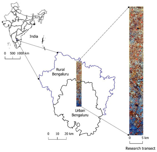
Figure 1.
Location of the study area in the northern part of Bengaluru District, Karnataka, India, showing a 5 km × 50 km transect. The transect is enlarged here as a WorldView-3 false-color composite.
2.2. Satellite Imagery
Remote sensing data from WorldView-3 and Landsat 8 from November 2016 were used. Both image sets were cloud-free and covered the same extent of 250 km2 (Figure 1). The high-resolution, pan-sharpened WorldView-3 imagery with 30 cm spatial resolution was used as the reference data set and served as a substitute for wall-to-wall “ground truthing.” Landsat 8 Surface Reflectance Tier 1 with a spatial resolution of 30 m served as input for the pixelwise tree cover prediction. To ensure the best possible spatial alignment, an image-to-image co-registration was done by automatic tie point extraction in PCI Geomatica® Banff (PCI Geomatics Enterprises, Inc., Markham, ON, Canada).
In addition, tree canopy coverage data were retrieved from the NASA Land-Cover/Land-Use Change Program. The ready-to-use Global Tree Canopy Cover product [11] with 30 m resolution was announced in May 2019 in Version 4 and was processed from the Landsat image archive. It shows the tree canopy coverage per pixel in the range between 0% and 100%.
2.3. Training Data
The training data were collected as values between 0% and 100% tree cover per pixel (Table 1). A systematic sample of n = 108 square plots of 1 ha area was established on the WorldView-3 imagery within the research transect to generate reference data as “ground truth.” In these square plots, only Landsat pixels completely inside the plot boundary were collected. The total of 970 training pixels constituted a good balance between time taken for collecting the training data and the large number of training data required as input for neural network based image classification. The systematic sampling approach ensured that the variability in tree cover within the study region was well represented. The systematic sample also produced an estimate of tree cover.

Table 1.
Distribution of training pixels over the 10% tree cover classes.
On each square plot, tree crowns were visually identified and delineated in the WorldView-3 imagery. Then, the tree crown shapefile was overlaid onto the vectorized Landsat-8 imagery. The latter step transformed each 30 m × 30 m Landsat pixel into a 30 m × 30 m single polygon. Using the geoprocessing tool “intersection” in Quantum GIS 3.10, the tree crown polygons within the borders of each pixel were cut out. For each pixel polygon, the corresponding percent tree cover was then calculated from this overlay. To complete the training data set, the spectral reflectance values from six Landsat 8 bands were assigned to each tree cover polygon. An overview of the variables of the training data set is given in Table 2.
Table 2.
List of variables used for the training data set.
2.4. Tree Cover Prediction
To predict continuous tree cover between 0 and 1 (corresponding to 0–100%), we used a Multilayer Perceptron (MLP) network; the workflow was implemented in Python using the TensorFlow package. MLP is a simple deep learning model that is trained via backpropagation and used for classification. In addition to the advantage that such neural networks can handle complexity well [26], the main reasons for using it were (1) the great variations in spectral reflectance for the tree cover per pixel, particularly for a tree cover smaller than 30%; and (2) the fact that we faced a non-linearity problem.
The structure of our fully connected network model consisted of two hidden layers with 16 neurons each. As we faced a regression problem, we used the root-mean-square error (RMSE) as a loss function together with the Adam optimizer [27] and the mean absolute error (MAE) as an accuracy metric. To monitor the performance and evaluate the model, we split our data into a training and validation dataset with 880 samples for the training, and we performed a 10-fold cross-validation. In each run, the network was fed another combination of training samples and was trained for 600 epochs, wherein a machine learning epoch means the number of cycles through the full training dataset.
3. Results
3.1. Spectral Reflectance Values
At first, we analyzed the range of spectral values and their relationship to tree cover percentage per pixel. Figure 2 shows the Pearson correlation coefficient for each one of the Landsat bands that were used as predictors. On the first visual assessment, the spread of spectral values (Figure 2) very well illustrated the inherent challenge we face when predicting continuous tree cover, particularly when it comes to lower tree cover percentage per pixel. Here, depending on the Landsat band, the ranges of spectral values varied, for example, between 200 to 800 (Band 2) and 1000 to 3000 (Band 6). For tree cover per pixel larger than 50%, however, the range of the spectral reflectance decreased more and more, as the land cover type “Trees” is the cover type that predominantly determines the spectral response. Landsat band 5 (the near-infrared band commonly used in vegetation analyses) showed the highest spectral variability over all values of tree cover percentage per pixel and no noticeable correlation (r = −0.01, p > 0.5). The highest correlation (r > 0.75) with tree cover percentage can be found for Landsat bands 3, 4 and 7.
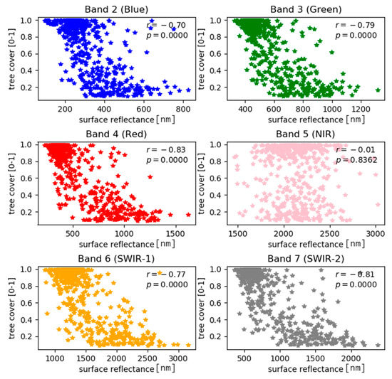
Figure 2.
Scatterplot of band-wise Landsat surface reflectance values (scale factor 0.001) against tree cover per pixel, where 0 equals 0% and 1 equals 100%.
Figure 3 illustrates the variation in the spectral response for a single Landsat pixel. Upon comparing the high-resolution WorldView-3 subsets (Figure 3a–c), we found that what all three examples had in common is that the percentage tree cover for the overlaid 30 m × 30 m Landsat pixel was within a range of 40–50%, in contrast with the surrounding landscape, which can cover impervious surfaces, agricultural land, barren land, etc. The resulting mixed pixels were strongly influenced by the varying land-cover conditions and led to different spectral signatures (Figure 3), which still had a similar percentage tree cover, a challenging situation for the classifier.
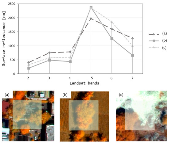
Figure 3.
(a–c) WorldView-3 imagery with overlaying 30 m × 30 m Landsat pixel with 40% to 50% tree cover and (on top) the corresponding spectral signature.
3.2. Continuous Map of Tree Cover
To produce the continuous tree cover map, the Landsat 8 satellite image was classified using a fully connected neural network classifier. Figure 4 shows the high-resolution WorldView-3 reference image, the tree cover density from the Global 30 m Landsat Tree Canopy Version 4, the predicted tree cover and the difference map side by side, and thus allows for a visual examination of the differences. We did a preliminary visual assessment of the map (Figure 4c), which suggested the densest tree cover mapped per pixel, for example, was in the historical Lalbagh Botanical Garden (Figure 4; red arrow). At the other end, the lowest tree cover was found in purely built-up areas. The 10-fold cross-validation indicated a mean absolute error (MAE) of 13.04% (±0.87%) as a measure of matching accuracy of the observed tree cover with the predicted tree cover.
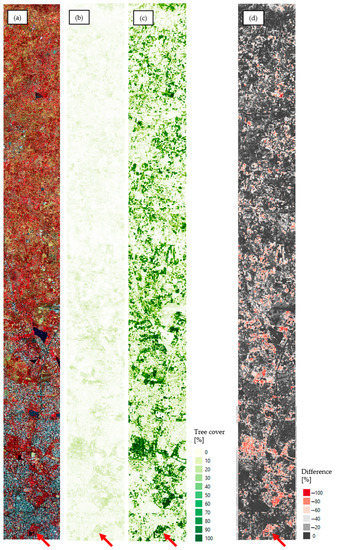
Figure 4.
(a) WorldView-3 false color composite (near infrared-red-green) from a subset of the study area. (b) Percent tree cover per pixel from the Global 30 m Landsat Tree Canopy Version 4 [13]. (c) Percent tree cover per pixel from Landsat-8 in our study. Legend is the same for (b,c). (d) Difference map: “global tree cover” (b) minus “our predicted product” (c).
Differences in tree cover become particularly visible when the saturation of greenness is compared. Results from the difference map (Figure 4d) show that there was an average underestimation of about 17.16% for the whole research transect. Areas which are characterized by solitary trees, roadside trees and groups of trees showed an underestimation of around 20–30%. A deviation in the range of 0 to 10% compared to our prediction was found in purely built-up areas where there was hardly any tree cover.
The overall systematic underestimation can be observed over the whole study area. The subset in Figure 5 gives a more detailed view of the differences. If focus is on the solitary and roadside trees, the global map that we used for comparison failed to predict low tree covers per pixel, so that these quite-abundant urban trees are not represented in the global map (Figure 5b). The neural network model, however, detected and predicted these types of urban trees, as well, which is indicated in Figure 5a by the white to light green pixels; the darker green pixels point to a higher percentage of tree cover, which indicates the presence of larger alley trees. The global tree canopy map predicted either no tree cover or an extremely small tree cover per pixel for the same area. Thus, the resulting map predicted by the neural network classifier also exhibited a much better local accuracy when applied at a regional level than the global map with which we compared our results.
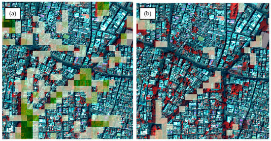
Figure 5.
600 m × 600 m subset of the WorldView-3 image from the urban parts of our study area, with alleys and solitary trees of varying crown size overlaid with (a) our predicted Landsat tree cover per pixel and (b) the Global 30 m Landsat Tree Canopy Version 4. The bright green pixels in (b) show a very low canopy cover, which obviously should be much higher when looking at the WorldView-3 image. Our prediction (a) shows a more reasonable canopy cover.
4. Discussion
We use and present an easy-to-implement neural network model to predict continuous tree cover percentage per pixel on Landsat imagery of urban tree cover. With the ability of neural networks to generalize well on the input data source, one can use the pretrained weights and fine-tune one’s own neural network model to predict urban tree cover from Landsat imagery in another region. Fine-tuning is an approach to transfer learning where a developed model is reused for a similar task: here, tree cover estimation in a different region. This method allows one to take advantage of what the model has already learned, which would considerably reduce the need to generate one’s own large training data set based on high-resolution images and to train a network from scratch.
The results show that there is considerable difference between the global product (Global 30 m Landsat Tree Canopy Version 4) and the predicted tree cover map from the neural network model, which outperforms the global map in terms of isolated trees, at least for our example of the study area of Bangalore (Figure 5). The global product, though also based on Landsat imagery, systematically and considerably underestimated the tree cover in this urban environment. Previous studies [11,28] have already shown that Landsat-derived tree cover estimates tend to systematically produce underestimations, particularly in areas with sparse tree cover. Even large parks with a closed canopy layer are not accurately predicted, with an actual tree cover per pixel of about 100%. The Global Forest Change data of Hansen et al. [10] for Bengaluru also seem to leave out a lot of areas (formerly) covered by trees despite offering canopy categories down to 10%. Only some scattered pixels are displayed within the city. It is obvious that there is still research as well as method development to be done in order to reliably map the urban tree cover of entire cities based on Landsat imagery.
The extreme differences found for the densely treed parks in Bangalore may be explained by the image selection used for creating the global map and hence the seasonal and phenological effects that cause the trees to be recognized differently. Because both our data sets were acquired in the same month, we did not need to consider this aspect further. Besides technical and processing reasons, the focus of the global maps tends to be on clusters of trees and patches of tree cover, like large forest areas, and takes less account of individually occurring trees that are typical in many rapidly urbanizing regions.
One aspect briefly mentioned in this study (Figure 3) is the object composition of a pixel and how this affects its spectral values. The same tree cover area might have very different spectral values depending on the distribution of the contained trees and their distances to each other and other objects. It is furthermore conceivable that neighboring buildings affect the spectral signature of trees differently compared to lower vegetation. That lower vegetation can influence the top-of-canopy reflectance was shown in a study looking at canopy cover estimation and the impact of understory reflectance [29]. In turn, a similar finding can be anticipated for urban trees, but with the difference that an overexposure from strongly reflecting roof materials can be expected. Further research should be conducted here to better understand how this influences the tree cover estimation.
An intrinsic problem, of course, with the use of images of different data sets and spatial resolutions is their geometrical misalignment [30]. Although the data sets have the same projection and coordinate reference system, misalignments between the Landsat-8 and WorldView-3 imagery are still to be expected and affect the accuracy of the model [31]. The problem is pervasive and hard to solve even though we used state-of-the-art processing in PCI Geomatica® Banff in this study. Consequently, we may still expect a systematic deviation of unknown size in the spectral values assigned to the tree cover per pixel. Such deviation will then also be reflected in the predicted tree cover. Without perfect co-registration, the location of the digitized canopies does not exactly match the extent of the pixel, and in turn, erroneous spectral values will be assigned.
5. Conclusions
Our continuous tree cover assessment from a fully connected network yielded a more plausible tree cover product for our study area on a regional scale (250 km2 in the Northern parts of the Bangalore Metropolitan Region) than a global map with which we compared our results. The new map of tree cover may provide a starting point for further research on larger area assessment and mapping of non-forest tree cover, as required, for example, for modelling biodiversity or researching the role of urban trees for mitigation of climate change. Among the immediately emerging topics for further research are (1) to compare the Landsat classification with WorldView-3 imagery and then derive a kind of “calibration function”; and (2) to apply our approach to historical Landsat imagery with the aim to monitor long-term changes of tree cover in urban environments and thus enhance data sets in monitoring programs.
Author Contributions
Conceptualization, methodology and writing—original draft, N.N. The author has read and agreed to the published version of the manuscript.
Funding
This research funded by the German Research Foundation, DFG, through grant number KL 894/23-2 and NO 1444/1-2 as part of the Research Unit FOR2432/2.
Acknowledgments
The author gratefully acknowledges the financial support provided by the German Research Foundation, DFG, through grant number KL 894/23-2 and NO 1444/1-2 as part of the Research Unit FOR2432/2. Great thanks go to the former student Marco Sendner, University of Göttingen, for his comprehensive support to the training data collection.
Conflicts of Interest
The author declares no conflict of interest.
References
- Lindenmayer, D.B.; Laurance, W.F.; Franklin, J.F. Global Decline in Large Old Trees. Science 2012, 338, 1305–1306. [Google Scholar] [CrossRef]
- Stagoll, K.; Lindenmayer, D.B.; Knight, E.; Fischer, J.; Manning, A.D. Large trees are keystone structures in urban parks. Conserv. Lett. 2012, 5, 115–122. [Google Scholar] [CrossRef]
- Holmgren, P.; Masakha, E.J.; Sjoholm, H. Not all African land is being degraded: A recent survey of trees on farms in Kenya reveals rapidly increasing forest resources. Ambio 1994, 23, 390–395. [Google Scholar]
- Kleinn, C. On large area inventory and assessment of trees outside forests. Unasylva 2000, 51, 3–10. [Google Scholar]
- Plieninger, T.; Hartel, T.; Martín-López, B.; Beaufoy, G.; Bergmeier, E.; Kirby, K.; Montero, M.J.; Moreno, G.; Oteros-Rozas, E.; Van Uytvanck, J. Wood-pastures of Europe: Geographic coverage, social–ecological values, conservation management, and policy implications. Biol. Conserv. 2015, 190, 70–79. [Google Scholar] [CrossRef]
- Lamb, D.; Stanturf, J.A.; Madsen, P. What Is Forest Landscape Restoration? In World Forests; Springer: Berlin/Heidelberg, Germany, 2012; Volume 15, pp. 3–23. [Google Scholar]
- Pandey, D. Trees outside the forest (TOF) resources in India. Int. For. Rev. 2008, 10, 125–133. [Google Scholar] [CrossRef]
- Karlson, M.; Ostwald, M.; Reese, H.; Sanou, J.; Tankoano, B.; Mattsson, E. Mapping Tree Canopy Cover and Aboveground Biomass in Sudano-Sahelian Woodlands Using Landsat 8 and Random Forest. Remote Sens. 2015, 7, 10017–10041. [Google Scholar] [CrossRef]
- Hunsinger, T.; Moskal, L.M. Half a Century of Spatial & Temporal Landscape Changes in the Finley River Basin, Missouri. In Proceedings of the Association of American Geographers Annual Conference, Denver, CO, USA, 5–9 April 2005. [Google Scholar]
- Hansen, M.C.; Potapov, P.V.; Moore, R.; Hancher, M.; Turubanova, S.A.; Tyukavina, A.; Thau, D.; Stehman, S.V.; Goetz, S.J.; Loveland, T.R.; et al. High-resolution global maps of 21st-century forest cover change. Science 2013, 342, 850–853. [Google Scholar] [CrossRef]
- Sexton, J.O.; Song, X.-P.; Feng, M.; Noojipady, P.; Anand, A.; Huang, C.; Kim, D.-H.; Collins, K.M.; Channan, S.; DiMiceli, C.; et al. Global, 30-m resolution continuous fields of tree cover: Landsat-based rescaling of MODIS vegetation continuous fields with lidar-based estimates of error. Int. J. Digit. Earth 2013, 6, 427–448. [Google Scholar] [CrossRef]
- Awuah, K.; Nölke, N.; Freudenberg, M.; Diwakara, B.; Tewari, V.P.; Kleinn, C. Spatial resolution and landscape structure along an urban-rural gradient: Do they relate to remote sensing classification accuracy?—A case study in the megacity of Bengaluru, India. Remote Sens. Appl. Soc. Environ. 2018, 12, 89–98. [Google Scholar] [CrossRef]
- Zhang, D.; Zheng, H.; Ren, Z.; Zhai, C.; Shen, G.; Mao, Z.; Wang, P.; He, X. Effects of forest type and urbanization on carbon storage of urban forests in Changchun, Northeast China. Chin. Geogr. Sci. 2015, 25, 147–158. [Google Scholar] [CrossRef]
- Alberti, M.; Weeks, R.; Coe, S. Urban Land-Cover Change Analysis in Central Puget Sound. Photogramm. Eng. Remote Sens. 2004, 70, 1043–1052. [Google Scholar] [CrossRef]
- Dopido, I.; Zortea, M.; Villa, A.; Plaza, A.; Gamba, P. Unmixing Prior to Supervised Classification of Remotely Sensed Hyperspectral Images. IEEE Geosci. Remote Sens. Lett. 2011, 8, 760–764. [Google Scholar] [CrossRef]
- Small, C. Estimation of urban vegetation abundance by spectral mixture analysis. Int. J. Remote Sens. 2001, 22, 1305–1334. [Google Scholar] [CrossRef]
- Zhang, J.; Foody, G.M. Fully-fuzzy supervised classification of sub-urban land cover from remotely sensed imagery: Statistical and artificial neural network approaches. Int. J. Remote Sens. 2001, 22, 615–628. [Google Scholar] [CrossRef]
- Zhu, X.X.; Tuia, D.; Mou, L.; Xia, G.-S.; Zhang, L.; Xu, F.; Fraundorfer, F. Deep Learning in Remote Sensing: A Comprehensive Review and List of Resources. IEEE Geosci. Remote Sens. Mag. 2017, 5, 8–36. [Google Scholar] [CrossRef]
- Ma, L.; Liu, Y.; Zhang, X.; Ye, Y.; Yin, G.; Johnson, B.A. Deep learning in remote sensing applications: A meta-analysis and review. ISPRS J. Photogramm. Remote Sens. 2019, 152, 166–177. [Google Scholar] [CrossRef]
- Sudhira, H.; Nagendra, H. Local assessment of Bangalore: Graying and greening in Bangalore—Impacts of ur-banization on ecosystems, ecosystem services and biodiversity. In Urbanization, Biodiversity and Ecosystem Services: Challenges and Opportunities; Elmqvist, T., Fragkias, M., Goodness, J., Güneralp, B., Marcotullio, P.J., McDonald, R.I., Parnell, S., Schewenius, M., Sendstad, M., Seto, K.C., et al., Eds.; Springer: Berlin/Heidelberg, Germany, 2013; pp. 75–91. [Google Scholar]
- World Population Review. Bangalore Population 2020 (Demographics, Maps, Graphs). 2020. Available online: http://worldpopulationreview.com/world-cities/bangalore-population (accessed on 2 November 2020).
- Nagendra, H.; Gopal, D. Street trees in Bangalore: Density, diversity, composition and distribution. Urban For. Urban Green. 2010, 9, 129–137. [Google Scholar] [CrossRef]
- Nair, J. The Promise of the Metropolis: Bangalore’s Twentieth Century; Oxford University Press: New Delhi, India, 2005. [Google Scholar]
- Sudhira, H.; Ramachandra, T.; Subrahmanya, M.B. Bangalore. Cities 2007, 24, 379–390. [Google Scholar] [CrossRef]
- Nagendra, H.; Nagendran, S.; Somajita, P.; Pareeth, S. Graying, greening and fragmentation in the rapidly expand-ing Indian city of Bangalore. Landsc. Urban Plan. 2012, 105, 400–406. [Google Scholar] [CrossRef]
- Venkatesh, Y.; Raja, S.K. On the classification of multispectral satellite images using the multilayer perceptron. Pattern Recognit. 2003, 36, 2161–2175. [Google Scholar] [CrossRef]
- Kingma, D.P.; Ba, J. Adam: A method for stochastic optimization. In Proceedings of the International Conference Learn. Represent. (ICLR), San Diego, CA, USA, 5–8 May 2015. [Google Scholar]
- Hansen, M.C.; DeFries, R.S.; Townshend, J.R.G.; Marufu, L.; Sohlberg, R. Development of a MODIS tree cover vali-dation data set for Western Province, Zambia. Remote Sens. Environ. 2002, 83, 320–335. [Google Scholar] [CrossRef]
- Landry, S.; St-Laurent, M.-H.; Nelson, P.R.; Pelletier, G.; Villard, M.-A. Canopy Cover Estimation from Landsat Images: Understory Impact onTop-of-canopy Reflectance in a Northern Hardwood Forest. Can. J. Remote Sens. 2018, 44, 435–446. [Google Scholar] [CrossRef]
- Dawn, S.; Saxena, V.; Sharma, B. Remote Sensing Image Registration Techniques: A Survey. In Abderrahim Elmoataz, Olivier Lezoray, Fathallah Nouboud, Driss Mammass und Jean Meunier (Hg.): Image and Signal Processing, 4th International Conference, ICISP 2010, Trois-Rivières, QC, Canada, 30 June–2 July 2010; Lecture Notes in Computer Science; Springer: Berlin, Germany, 2010; Volume 6134, pp. S103–S112. [Google Scholar]
- Pohl, C. Tools and methods for fusion of images of different spatial resolution. Int. Arch. Photogramm. Remote Sens. 1999, 32. Available online: www.researchgate.net/publication/228832484_Tools_and_Methods_for_Fusion_of_Images_of_Different_Spatial_Resolution (accessed on 8 October 2020). [CrossRef]
Publisher’s Note: MDPI stays neutral with regard to jurisdictional claims in published maps and institutional affiliations. |
© 2021 by the author. Licensee MDPI, Basel, Switzerland. This article is an open access article distributed under the terms and conditions of the Creative Commons Attribution (CC BY) license (http://creativecommons.org/licenses/by/4.0/).