Meeting Challenges in Forestry: Improving Performance and Competitiveness

Abstract

Improving the efficiency of the forestry sector will have an important impact on our possibility to attain long-term sustainability and mitigate climate change. In this study, attainable, and sustainable, efficiency improvements in the harvesting of forest products are analyzed using Data Envelopment Analysis (DEA). The price impacts of the efficient harvesting volumes are evaluated in a second step using a spatial forest sector model. The results indicate that the harvested volumes of forest products, both for the industry and energy sectors, can be significantly increased if a more efficient forest management is adopted. This supply-side effect will also result in general price decreases for sawlogs, pulpwood, fuelwood and harvesting residues. However, in certain counties, and for specific forest products, the estimated decreasing price effect from a more efficient forest management cannot fully offset the increasing price effect of the energy sector expanding its use of forest products. More forest biomass enters the market, which is needed in the transition towards a bioeconomy, and the increased availability of forest biomass will restrict the price effect making investments in the bioeconomy more likely to be profitable.

1. Introduction

The forest sector is usually an economically important sector in forest endowed countries [1]. As such, it is important to evaluate the performance of the sector to ensure a high efficiency and competitiveness as well as to provide knowledge for continuous improvements. In addition, climate change mitigation, provision of ecosystem services, recreation and renewable energy as well as suppling feedstocks to a growing bioeconomy are but a few of the challenges facing the forest sector today, while surrounded by stringent sustainability issues. The success of the forest sector to meet these challenges depends on improving its performance and competitiveness, as well as on developing new products, developing new or improved technologies and on the ability to adapt to changing market conditions (e.g., [2]).

The purpose of this study is to evaluate price impacts of attainable, and sustainable, efficiency improvements in the harvesting of forest products. To achieve this purpose, an integrated approach of two forest models is proposed. The first model explicitly addresses the efficiency issues in the forestry sector using a Data Envelopment Analysis (DEA) approach. The second model exploits the obtained results in a partial equilibrium forest sector model to estimate price effects with the improved performances. This paper is the first one analyzing effects from an improved performance in the forestry sector by integrating these two methodologies.

There are several methods available to evaluate the performance and competitiveness of the forest sector. Performance is commonly measured as efficiency using different DEA techniques. This approach, applied to forestry, has received some attention in the scientific literature (for a review see [3]). Commonly, the efficiency of geographical delimited areas is analyzed based on the argument that they exhibit differences in e.g., timber production, soil conservation and forest recreation. In a series of papers, the regional efficiency of Taiwanese forest districts is evaluated. This includes reorganization issues [4,5,6], forest management [7], multiple-output [8], parallel production units [9] and physical and organizational congestion [10]. For China, the efficiency of implementing forest protection programs in ten regions in Western China is analyzed [11] and the forest resources efficiency of 31 inland Chinese provinces is evaluated [12]. The latter study is expanded [13] by including carbon sequestration as a desirable output. The efficiency scores for 19 regional Forestry Boards in Finland are computed [14] and on a larger geographical scale, the efficiency for European member states is evaluated [15]. A comparison of efficiency between the Slovak forestry sector with other European countries is made [16]. For British Columbia (Canada), the efficiency of timber allocation to sawmills from 58 stewardship units (i.e., forested areas) is assessed [17]. Non-provisional ecosystem services as output variables are included in the analyses of three management systems at stand level in Finland to illustrate trade-offs between timber products and ecosystem services [18]. Eco-efficiency has been studied in terms of undesirable outputs [19]. The efficiency of logging operations in New Zealand has been investigated using data on unique forest harvest operations [20,21]. The efficiency of planted forest plots in Florida (USA) in providing timber, carbon sequestration and tree species richness has been evaluated [22]. In addition, managerial issues have been studied addressing the relationship between institutional and managerial practices and efficiency [23].

Competitiveness is a vaguer concept and thus harder to measure. However, price effects and changing resource allocation patterns are ways to measure relative changes in competitiveness. This approach can be implemented in Forest Sectors Models (FSM) using a partial equilibrium framework (for reviews see [2,24,25]). Most FSM rely on the modelling framework developed by the Global Forest Sector Model [26,27,28] and have been applied on a global dimension (e.g., [26]), national dimension (e.g., [29]), national multi-spatial dimension (e.g., [30,31]) and multi-spatial transnational dimension (e.g., [32]). They have also been used to analyze the effects of increased forest conservation and general environmental considerations (e.g., [33]), increased energy production utilizing forest biomass (e.g., [34]), forecasting future price developments (e.g., [35]), changing trade conditions (e.g., [36]), changes to the forest inventory (e.g., [37]), and the optimal location for the establishment of new industries/mills (e.g., [38]).

In this paper, the performance and competitiveness of the forest sector is evaluated by combing these approaches (i.e., DEA and FSM). As such, our study contributes to the literature on sector-level impacts of improved forest harvesting efficiencies by analyzing the performance of the Swedish forest sector, by specifically evaluating the market impacts from an improved efficiency of forest biofuel production, and by integrating two methodological approach.

2. Materials and Methods

The methodological approach is based on an integrated two-step process. In the first step, the performance of the Swedish forest sector on county level is estimated using a novel Data Envelopment Analysis (DEA) technique. DEA is a linear programming, non-parametric analytical technique that measures the relative efficiency of comparable organizational units (decision-making unit or DMU) in transforming certain inputs into certain outputs. In this setting, the objective is to evaluate by how much the individual counties can be expected to increase their harvesting volumes of forest products by using the same volume of inputs more efficiently. This is especially important in the management of scarce natural resources. In the second step, the estimated efficient harvesting volumes are used in a partial equilibrium Forest Sector Model (FSM). This approach is used to analyze competitiveness of the forest sector in terms of price and resource allocation effects. The model results provide a comprehensive account on how the forest sector is affected by a change to base-line situation (business-as-usual). The FSM is solved as a non-linear optimization problem under several restrictions. In our case, the aim is to maximize the economic welfare from the utilization of available forest resources before and after a more efficient forestry.

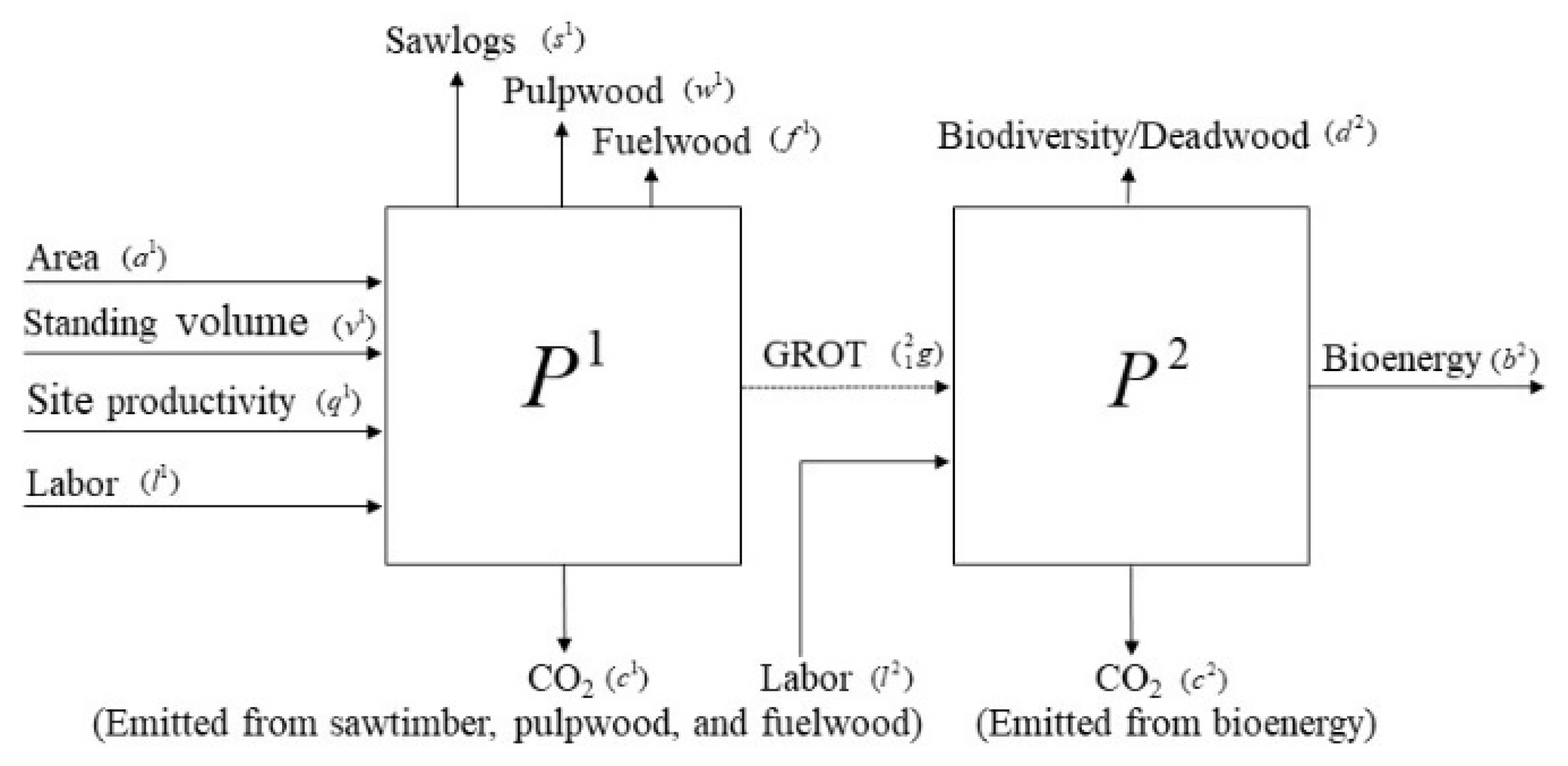
2.1. Efficiency Estimation (Network DEA)

A network DEA approach is applied to measure the forest bioenergy production efficiency (for more details on the production technology modelling see [39]). In the Appendix A, detailed descriptions of the two production technologies, the DEA model specification, variable definitions and unit of measurement are presented. In this section, we briefly explain the methodological framework. The DEA approach is suitable for our purposes in this study since it can capture the multi-production technology which underlies forest management decisions. It can also take into account both good and bad outputs (desirables and undesirables). In our case we can allow the technology to include biodiversity (deadwood as proxy), carbon sequestration and carbon emissions from bioenergy combustion. The approach is conceptually outlined in Figure 1, and below we describe the technology and our assumptions.

It is assumed that there are two production technologies: primary production $\left(P^1\right)$ and bioenergy production $\left(P^2\right)$. Let $x^1=\left(a^1,q^1,v^1,l^1\right)$ denote inputs into primary production, which include land area $\left(a^1\right)$, standing volume $\left(v^1\right)$, site productivity $\left(q^1\right)$ and labor $\left(l^1\right)$. Let $y^1=\left(s^1,w^1,f^1\right)$ denote primary production outputs, which include sawlogs $\left(s^1\right)$, pulpwood $\left(w^1\right)$ and fuelwood $\left(f^1\right).$ In addition, as the link between the two production technologies, harvetsing residues (GROT) is included and denoted by $g^1$. Finally, the primary production also generates undesirable CO₂ emissions $\left(c^1\right)$. The primary production technology $\left(P^1\right)$ is defined as:

$$P^1\left(x^1\right)=\left\{\left(y^1,g^1,c^1\right):x^1 \mathrm{can} \mathrm{produce} y^1,g^1 \mathrm{and} c^1\right\}$$

(1)

The harvesting residue output $\left(g^1\right)$ from primary prodiction $\left(P^1\right)$ enters as an input into the bioenergy production $\left(P^2\right)$. Thus, let $x^2=\left(g^1,l^2\right)$ denote inputs for the bioenergy production $\left(P^2\right)$ and $y^2=\left(b^2,d^2\right)$ its output, where $b^2$ is the bioenergy output and $d^2$ is a biodiversity measure (proxied by the amount of deadwood). Finally, the bioenergy production also have CO₂ emissions $\left(c^2\right).$ The bioenergy production technology $\left(P^2\right)$ as:

$$P^2\left(x^2\right)=\left\{\left(y^2,c^2\right):x^2 \mathrm{can} \mathrm{produce} y^2 \mathrm{and} c^2\right\}$$

(2)

The observed revenue for decision-making unit $k$ is expressed as:

$$R_k={\displaystyle \sum }{p}_k^f{y}_k^1+p_k^b{b}_k^2+p_c{C}_a^k-p_c\left(c^1+c^2\right)$$

(3)

where $C_a$ is amount of carbon sequestered in annual growth, vector $p^y$denotes prices associated with sawtimber, pulpwood and fuelwood, $p^b$ denotes the price associated with biofuel and $p^c$ is CO₂ price.

The revenue efficiency is defined as $\beta =R_k^{*}/R_k$, where $R_k$ and $R_k^{*}$ denotes the observed and the optimal revenue from forestry outputs, respectively. If ${\beta }_k=1$, then the harvesting operation is efficient and inefficient if ${\beta }_k>1$. The revenue efficiency measure is output oriented and includes both technical and allocative inefficiency. We are not interested in separating these two types of inefficiencies in the present study as we are mostly concerned with overall ineffiency and how resolving these inefficiencies would affect market conditions (e.g., prices of forest products) and sustainability (biodiversity and carbon sequestration).

The empirical implementation is based on estimating an efficiency score for each county by solving a linear programming maximization problem. The objective is to maximize the net revenue from outputs, including sawlogs $\left(s^1\right)$, pulpwood $\left(w^1\right)$, fuelwood $\left(f^1\right)$ and carbon sequestration $\left(C_a\right)$, minus the payment to carbon emissions $\left(c^1 \mathrm{and} c^2\right)$. The inputs, including land area $\left(a^1\right)$ and standing volume $\left(v^1\right)$, are specified to be no more than the observed values (see Appendix A).

The primary production technology $\left(P^1\right)$ is assumed to have variable returns to scale (VRS) since there is a limit to scaling up the site productivity. The bioenergy production technology $\left(P^2\right)$ is assumed to have non-deceasing returns to scale (NRS), which implies nonnegative profits [40]. In addition, constraints are added to both technologies specifying strong disposability for desirable outputs and weak disposability for CO₂ emissions. In other words, producers can always harvest less biomass and produce fewer primary outputs but reducing CO₂ emissions is costly in the sense that it can only be done by simultaneously reducing $y^1$ proportionally, while holding the inputs fixed [40].

Finally, two more restrictions are added. A maximum of 80 percent of the harvesting residues can be harvested as bioenergy (a formal regulation in Sweden) and that the amount of deadwood is not allowed to decline. Deadwood output is not required to follow the feature of weak disposability. Reducing CO₂ emissions (from combustion of bioenergy) require reducing the volume of harvesting residues being extracted, as such, the amount of deadwood may not certainly decrease.

2.2. Partial Equilibrium Forest Model

The FSM developed is a static, one-period optimization model, where the objective function is to maximize the total economic well-being (i.e., economic welfare) across the counties, given several constraints (for a detailed outline and description of the model see [31,41]). For competitive markets, this is equivalent to maximizing the sum of the consumer and producer surpluses, minus the total cost of inter-regional trade (cf. Equation (4)). The model is built on the assumption that industries use a Leontief production function (e.g., [26]). The model is implemented in General Algebraic Model System (GAMS) and solved using the CONOPT solver.

The model is expressed as:

$$\begin{gathered} \max {\displaystyle \sum }_{i,o}{{\displaystyle \int }}_l^Q\left(p_{i,o}{\left(\frac{Q_{i,o}}{q_{i,o}}\right)}^{\frac{1}{{\xi }_{i,o}}}\right)d{Q}_{i,o} \\ -{\displaystyle \sum }_{i,RW}{{\displaystyle \int }}_0^H\left(a_{i,RW}+{\omega }_{i,RW}{H}_{i,RW}^{{\epsilon }_{i,RW}}\right)d{H}_{i,RW} \\ -{\displaystyle \sum }_{i,HR}{{\displaystyle \int }}_0^R\left(b_{i,HR}+\frac{{{\displaystyle \sum }}_{RW}{h}_{i,RW}}{{{\displaystyle \sum }}_{i,RW}{H}_{i,RW}}{\rho }_{i,HR}{R}_{i,HR}^{{\mu }_{i,HR}}\right)d{R}_{i,HR} \\ -{\displaystyle \sum }_{IM,EX,T}\left(t{c}_{IM,EX,T}T{R}_{IM,EX,T}\right) \end{gathered}$$

(4)

s.t.

$$Q_{i,o}-{\displaystyle \sum }_{AC}\left({\theta }_{i,AC,o}{X}_{i,AC}\right)+{\displaystyle \sum }_{IM}T{R}_{i,IM,o}-{\displaystyle \sum }_{EX}T{R}_{i,EX,o}=0$$

(5)

$$-{\displaystyle \sum }_{AC}\left({\theta }_{i,AC,RW}{X}_{i,AC}\right)-H_{i,RW}+{\displaystyle \sum }_{IM}T{R}_{i,IM,RW}-{\displaystyle \sum }_{EX}T{R}_{i,EX,RW}=0$$

(6)

$$-{\displaystyle \sum }_{AC}\left({\theta }_{i,AC,HR}{X}_{i,AC}\right)-R_{i,HR}+{\displaystyle \sum }_{IM}T{R}_{i,IM,HR}-{\displaystyle \sum }_{EX}T{R}_{i,EX,HR}=0$$

(7)

$$-{\displaystyle \sum }_{ByC}\left({\theta }_{i,ByC}{X}_{i,ByC}\right)+{\displaystyle \sum }_{IM}T{R}_{i,IM,BP}-{\displaystyle \sum }_{EX}T{R}_{i,EX,BP}\ge {\displaystyle \sum }_{ByP}\left({\theta }_{i,ByP,BP}{X}_{i,ByP}\right)$$

(8)

$$Q_{i,o}\le q_{i,o}; H_{i,RW}\le h_{i,RW}; R_{i,RW}\le r_{i,RW}; X_{i,AC}\le k_{i,AC}$$

(9)

where $i$ denotes county, $o$ is end-product, $RW$ is roundwood assortment, $HR$ is harvesting residues, $BP$ is by-products (intermediate products), $T$ is tradable goods, and $l$ is the lower integral value for the end-products. $IM$ and $EX$ are subsets of $i$ and denote importing and exporting county, respectively. The set $AC$ denotes production activity (i.e., production technology) while $ByC$, and $ByP$ denote by-products consumers and producers as subsets of $AC$. The variable notation $H$ is roundwood harvesting rate, $R$ is extraction rate of harvesting residues, $Q$ is consumption of end-products, $X$ is utilization of woody inputs, and $TR$ is traded volumes. The parameter notation $a$ and $b$ are the reservation prices for roundwood and harvesting residues, respectively. Observed harvesting rate of roundwood is denoted by $h$, observed prices by $p$, observed consumption of end-products by $q$, and observed extraction rate of harvesting residues by $r$. The unit transportation cost is denoted by $tc$, and $k$ is the forest industry capacity constraint. $\xi$ is the own-price elasticity of end- product, $\epsilon$ is the inverse supply elasticity of roundwood supply, and $\mu$ inverse supply elasticity of harvesting residues (see Appendix A for an elaborate notation description and parameter values).

The inverse supply elasticities of roundwood $\left(\epsilon \right)$ and the harvesting residues $\left(\mu \right)$ are adjusted with respect to the observed regional price $\left(p\right)$ and the regional reservation price $\left(a \mathrm{or} b\right)$, thereby allowing for the possibility to calculate county specific elasticities (e.g., [26,30,42]).

$${\epsilon }_{i,RW}=\frac{1}{{\eta }_{i,RW}}\left(\frac{p_{i,RW}}{p_{i,RW}-a_{i,RW}}\right)$$

(10)

$${\mu }_{i,HR}=\frac{1}{{\nu }_{i,HR}}\left(\frac{p_{i,HR}}{p_{i,HR}-b_{i,HR}}\right)$$

(11)

In Equation (4), the first term is the sum of consumer surpluses from the end-products and the second term is the sum of producer surpluses from roundwood assortments, this includes sawlogs, pulpwood and fuelwood. The third term is the sum of producer surpluses from harvesting residues and the fourth term captures the reduced welfare from the costs associated with inter-regional trade.

Equation (5) states that consumption in each county must equal production net of trade. This constraint also ensure that all produced products will be consumed. Equation (6) states that roundwood demand is satisfied through county roundwood harvest or trade. Equation (7) states the same but for harvesting residues. Equation (8) states that by-product demand is less or equal to its supply, thus allowing for surplus supply but not surplus demand. Finally, Equation (9) states that there exists an upper limit (constraint) for end-product demand, roundwood harvest, extraction of harvesting residues and an upper capacity constraint for production units (i.e., activities).

The marginal effect of the balance constraints for roundwood (Equation (6)), for harvesting residues (Equation (7)) and for by-products (Equation (8)) gives the shadow price for the feedstock in each county [43]. The derived shadow prices from a more efficient forestry sector are assessed in comparison to a business-as-usual scenario (BAU), i.e., with current efficiency levels.

2.3. Data

Sweden has about 22.4 million hectare of productive forest land; the average annual standing volume is about 3.0 billion m³ standing volume; the average annual growth is about 116 million m³ standing volume. The average annual growth per hectare of the productive forest land, i.e., site quality, is about 6.9 m³ standing volume, with the lowest 2.9 m³ in the county of Norrbotten (far north) and the highest 11.2 m³ in county of Skåne (far south). The total removals of harvesting residues over the years 2008–2014 is 57.8 million m³s, with an average annual removal of about 8.3 million m³s.

The main output from the forestry sector is sawtimber, pulpwood, fuelwood and harvesting residues. These are the integrating variables for the two-step method outlined. In addition, the FSM includes woodchips, dry chips, sawdust and bark as by-products (intermediate products). The integrated models are implemented on 20 counties in Sweden (the island and county of Gotland is not included). Descriptive statistics and unit of measurement are outlined in the Appendix A.

The data used is obtained from the statistical database from the Swedish Forest Agency (SFA) [44], and the database of the Swedish National Forest Inventory (NFI) [45]. The data covers the years 2008 to 2014. The volumes of sawtimber, pulpwood and fuelwood produced in a county are obtained by multiplying the final felling volume in the county by the share of sawtimber, pulpwood and fuelwood of gross final felling, respectively. The shares of the three outputs are calculated using data on gross felling by region, assortment of stem wood and year. The volume of harvesting residues is obtained by multiplying the final felling volume in the county by the share of harvesting residues of gross final felling. The share of harvesting residues is calculated using data on annual total amount of harvesting residues distributed by felling and data on annual gross final felling, which is used by the national forest impact assessment by SFA [46]. The share of by-products of sawtimber and pulpwood used as energy is calculated using data from Biometria [47]. The biomass of pulpwood that is used as energy includes the bark of pulpwood, and the black liquor generated in chemical pulp process. It is estimated that 50% wood in weight would be burned as black liquor. Data on the cost of extracting harvesting residues comes from Skogforsk [48]. Prices for sawtimber and pulpwood are the annual volume weight average prices for delivery sawtimber and pulpwood [44]. Prices for fuelwood and prices for bioenergy (extracted harvesting residues) are wood chips price in SEK/MWh delivered to district heating [44]. In addition, the social cost of carbon is used as CO₂ price and set to 200 SEK per ton CO₂ [49]. All prices and costs are in 2015 SEK.

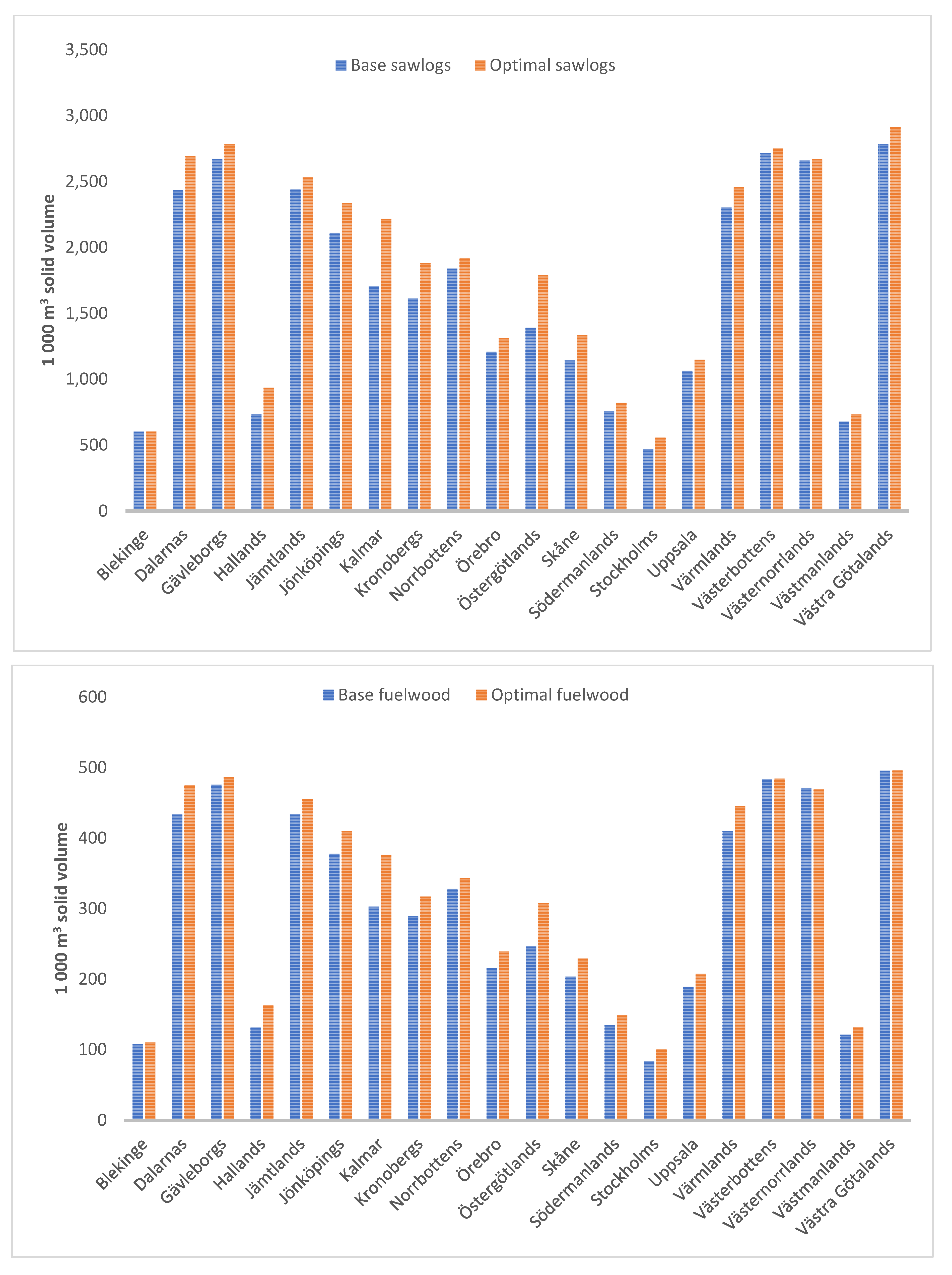
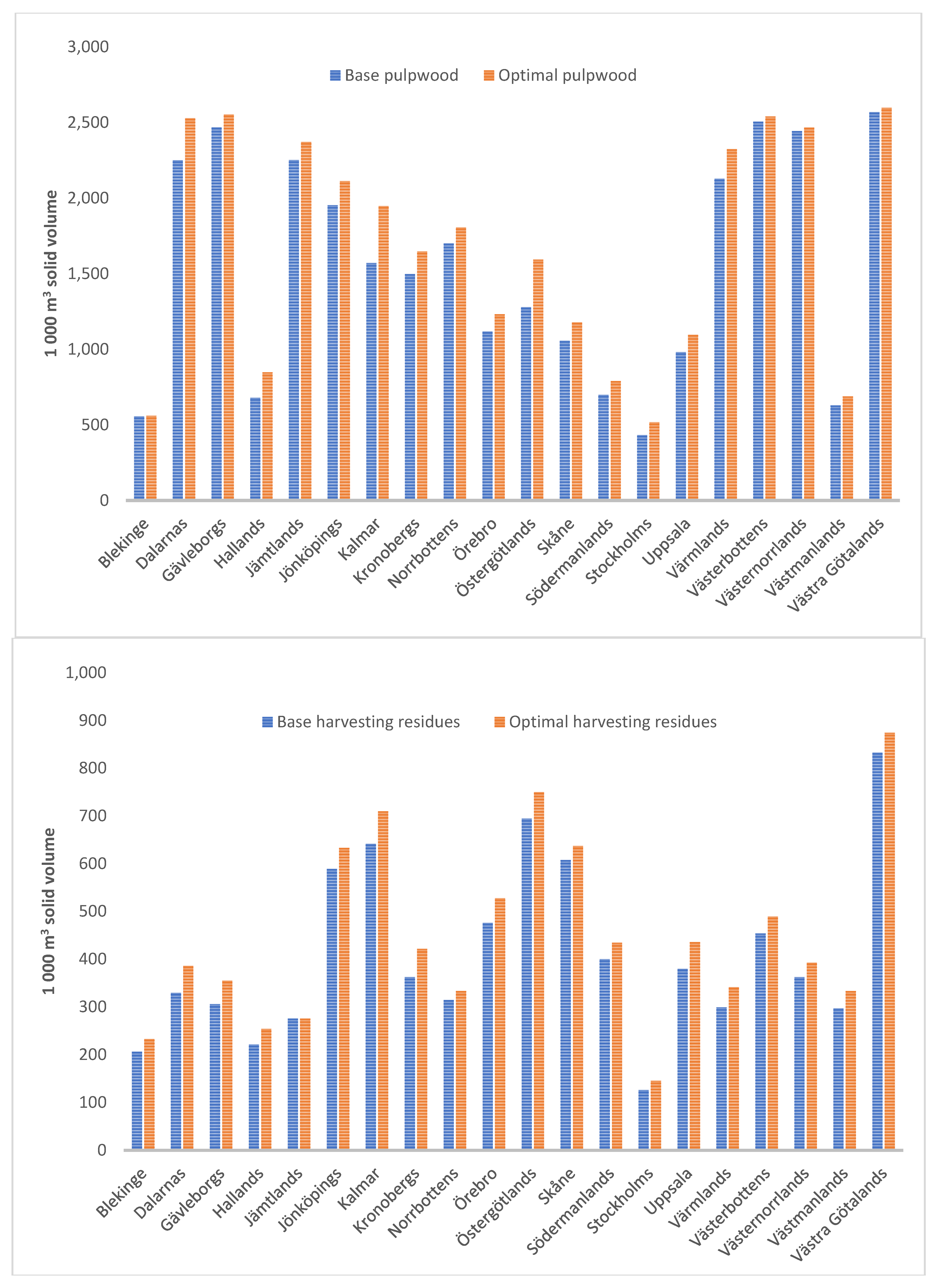
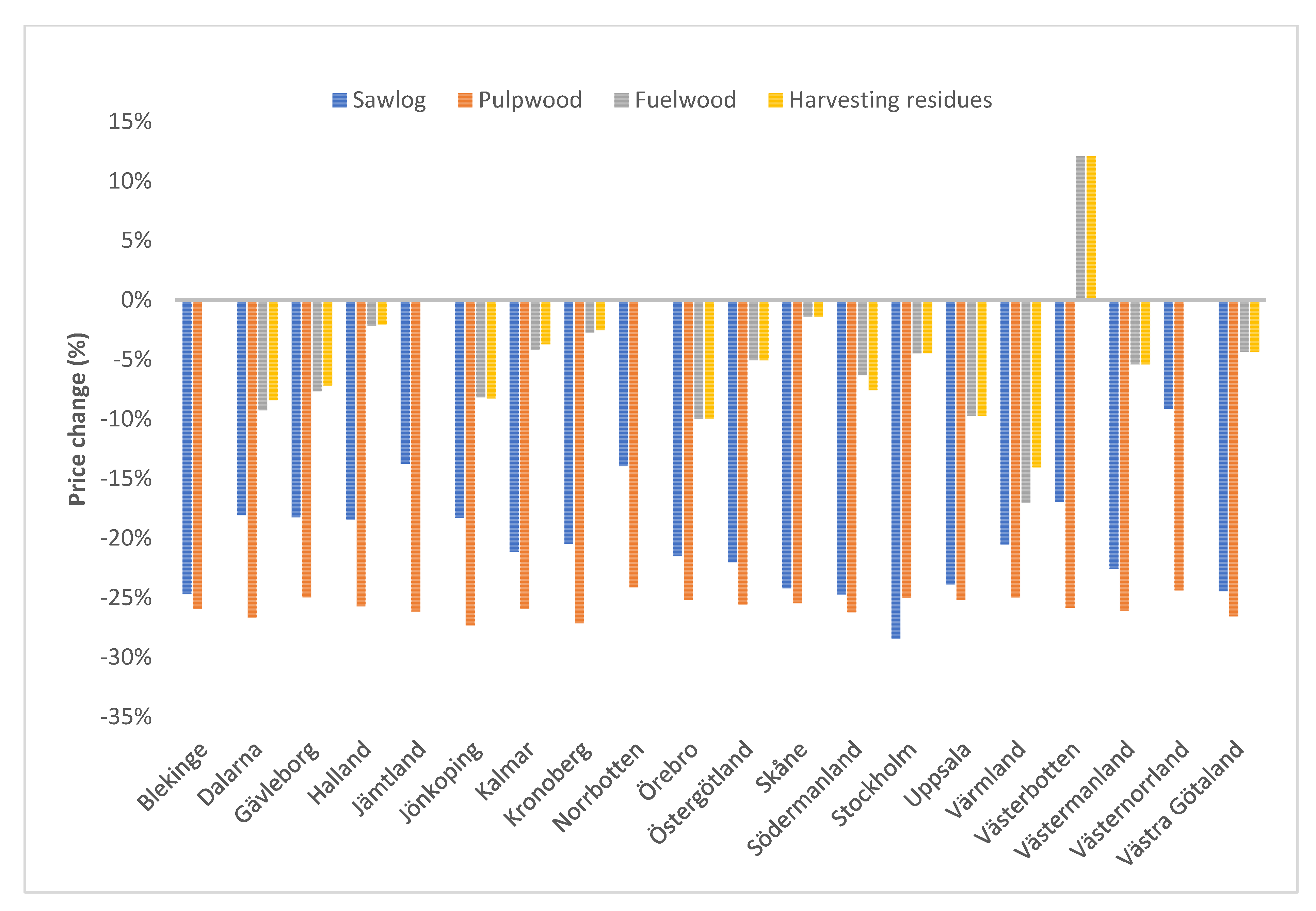
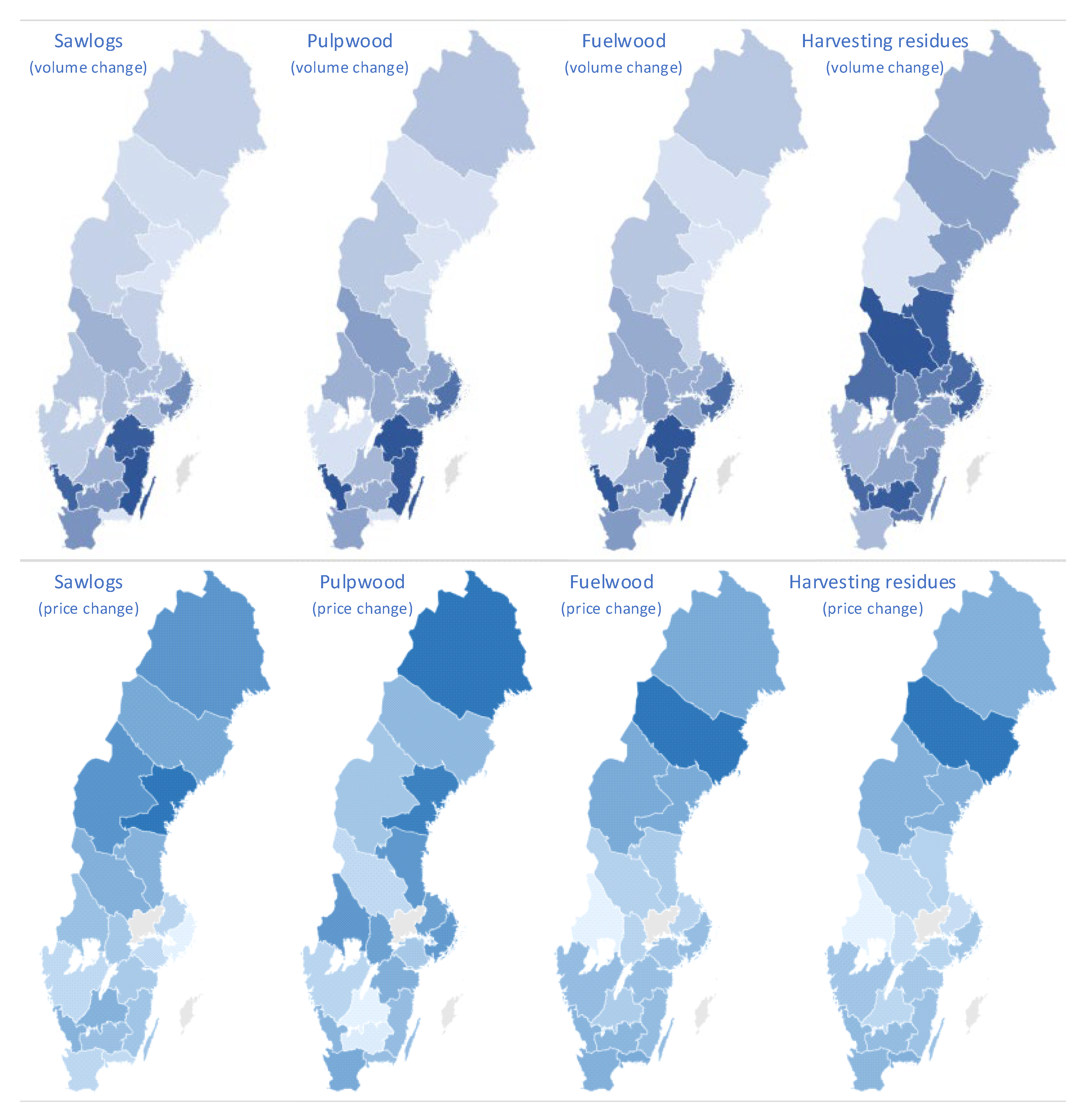
3. Results and Discussion

In a first step, the network DEA model is solved to estimated efficient harvesting levels and in a second step the FSM model is solved to estimate the price effects, using the average efficient volumes estimated by the network DEA model.

The revenue efficiency of bioenergy production is estimated for each county by solving the network DEA model and by using observations separately by year. As indicated in

Table 1. Average volume and price changes due to more efficient harvesting operations

Forest Product	Average Volume Change (DEA)	Average Price Change (FSM)
Sawlogs	9.2	−20.3
Pulpwood	8.5	−25.8
Fuelwood	7.8	−4.3
Harvesting residues	9.7	−4.1

, the overall results suggest that by improving the efficiency of the Swedish forestry sector, the harvesting of sawlogs can, on average over counties and over the studied time-period, increase by 9.2 percent (or by 152,878 m³ solid volume). The corresponding result for pulpwood is 8.5 percent (131,116 m³ solid volume), for fuelwood 7.8 percent (23,195 m³ solid volume) and for harvesting residues 9.7 percent (39,473 m³ solid volume).

By using the estimated efficient (optimal) harvesting volumes in the FSM, the implied price changes can be derived. These price changes are in relation to the business-as-usual, i.e., observed (inefficient) level of harvesting. Moreover, the results should be interpreted as a single effect analysis (ceteris paribus), i.e., how the price of the forest products would be affected if their supply would increase as suggested by the results of the network DEA model without any other changes. Thus, the results are not to be interpreted as a price forecast. As indicated in Table 1, the results suggest that the average price of sawlogs across counties would decrease by 20.3 percent because of more efficient harvesting operations. The corresponding price change for pulpwood is 25.8 percent, for fuelwood 4.3 percent and for harvesting residues 4.1 percent.

Results are also available on county level. Figure 2 presents the observed (base value) and efficient (optimal value) harvesting levels for the four wood assortments by county (average over the time-period) (the complete data for the results is presented in the Appendix A). For sawlogs, the largest (lowest) percentage increase in harvesting is achievable in the county of Kalmar (Blekinge) where the sawlog harvest can increase by more than 30 percent (0.2 percent) if the most efficient practice is used. In addition to Blekinge, the counties of Västernorrland and Västerbotten also show small increase potentials (i.e., the harvesting level of sawlogs are already close to the efficient level). For pulpwood, the corresponding largest (lowest) increase can be achieved in the county of Östergötland (Blekinge) where the pulpwood harvest can increase by approximately 24.5 percent (0.7 percent). The counties of Västra Götaland, Västernorrland and Västerbotten also have low increase potentials. Östergötland is also the county that can increase their harvest of fuelwood the most, by almost 25 percent. On the other hand, the results indicate that the county of Västernorrland need to reduce their harvest of fuelwood by 0.3 percent to become efficient. Thus, the fuelwood resources are currently slightly overexploited in Västernorrland. However, this result is well within the margin of error. The counties of Västra Götaland and Västerbotten also have a harvesting level of fuelwood that is close to the efficient level. Finally, the extraction of harvesting residues can increase by 17 percent in the county of Dalarna while the results suggest that the extraction level in Jämtland county is already efficient. However, harvesting residues is the product that has the potential to have the highest increase in most counties.

Figure 3 illustrate the price effect on county level from more efficient harvesting operations, i.e., if estimated increases in harvesting volumes becomes available. For sawlogs, the largest price decrease can be observed in Stockholm county (28 percent) followed by two cluster of counties that will experience price reduction around 22 and 16 percent. The smallest price decrease will occur in Västernorrland (9 percent). For pulpwood, the price effect is more constant around 25 percent for all counties. The price effect for fuelwood exhibits a larger dispersion between counties. For instance, the counties of Västernorrland, Norrbotten, Jämtland and Blekinge will not see any price effects on fuelwood from more efficient harvesting operations, while the county of Värmland will exhibit a 17 percent price effect. The other counties will have a price effect between two and ten percent, except for Västerbotten. The results for the county of Västerbotten suggest that the price of fuelwood and harvesting residues would increase as a consequence of more efficient harvesting operations. This results can be explained partly by relatively low observed price levels (starting price values) and partly by the changes in the allocation of use of forest products in neighboruring counties. That is, the price level in Västerbotten county is alligning with the price level in neighbouring counties. Finally, the increase in extraction level of harvesting residues suggest price effect like that of fuelwood but on a general lower level, e.g., the price effect on harvesting residues in the county of Värmland is 14 percent.

As indicated in Figure 4, the spatial variations in harvesting levels and price effects are high. However, some spatial clusters can be identified. For instance, the largest harvesting increases of stem wood (sawlogs, pulpwood and fuelwood) can be achieved in the coastal counties southeast and southwest of Sweden while the potential to increase the extraction of harvesting residues can be achieved further north and inlands.

Interestingly, the estimated price effects exhibit a different spatial pattern. The results suggest that the largest price effects will occur in the northern parts of Sweden for all four products (with some exceptions). This could be an indication that increasing harvesting volumes in northern Sweden is not meet by increasing demand to the same extent as in the southern parts of the county. That is, the results suggest a unilateral change on the supply side of the products markets.

To our knowledge, there are no similar studies directly comparable to ours. However, [4,5,6,7,8] analyze efficiency in Taiwan forest management, but with very different objectives. Our study is mainly focused on the market effects from reducing profit inefficiency. In actuality, [4,5,6,7,8] mainly focus on the technical efficiency without considering bad outputs or sustainability issues. However, in line with [4,5,6,7,8], we also find that there are significant inefficiencies in the production of conventional forest products.

4. Conclusions

This study estimates price impacts of attainable, and sustainable, efficiency improvements in the harvesting of forest products by developing and integrating two commonly used methods, namely data envelopment analysis (DEA) and partial equilibrium forest sector model (FSM). The DEA explicitly addresses the efficiency issues in the forestry sector while the FSM uses the DEA results to estimate the price effects an improved efficiency would result in.

Three positive effects can be identified. Firstly, more forest biomass enters the market, which is needed in the transition towards a bioeconomy, and secondly the increased availability of forest biomass will restrict the price effect making investments in the bioeconomy more likely to be profitable. Finally, by improving the efficiency, it is also possible to increase the harvested volumes without the need to increase the land area harvested, thus having a positive effect on several other ecosystem services provided by the forests.

A continuously increasing demand for forest resources, including ecosystem services such as carbon sequestration and recreation, coupled with the insight that it is not possible to increase the harvesting levels without jeopardizing long-run sustainability, will unintentionally only result in price increases and the same amount of forest resources is simply reallocated between different areas of utilization. However, the main conclusion based on the results in this paper is that the harvested volumes of forest products, both for the industry and energy sectors, can be significantly increased if a more efficient forest management is adopted. This supply-side effect will also result in general price decreases for sawlogs, pulpwood, fuelwood and harvesting residues. However, in certain counties, and for specific forest products, the estimated decreasing price effect from a more efficient forest management cannot fully offset the increasing price effect of the energy sector expanding its use of forest products. This suggests that spatial considerations are important to make appropriate conclusions regarding the price effect.

Measures should be taken to improve the efficiency of harvesting operations. This will not only improve the economics of the forest industry and bioenergy sector, but it will also facilitate the possibility to increase biodiversity and other ecosystem services without increasing the resource competition. The potential for expanding the use of the forest products is most beneficial in the Northern part of Sweden. This part of the Sweden will experience the largest price effect (a downward pressure on the forest product prices) suggesting untapped reserves of forest products. However, based on the average price changes, a more efficient forest management will generate larger price effects in traditional forest products (sawlogs and pulpwood used in the forest industry) compared to biofuels (fuelwood and harvesting residues) used for energy. Consequently, especially pulpwood will become a more interesting fuel option for the energy sector, increasing the feed-stock competition.

References

1. Li, Y.; Mei, B.; Linhares-Juvenal, T. The economic contribution of the worldߣs forest sector. For. Policy Econ. 2019, 100, 236–253. [Google Scholar] [CrossRef]
2. Hurmekoski, E.; Hetemäki, L. Studying the future of the forest sector: Review and implications for long-term outlook studies. For. Policy Econ. 2013, 34, 17–29. [Google Scholar] [CrossRef]
3. Sowlati, T. Efficiency studies in forestry using data envelopment analysis. For. Prod. J. 2005, 55, 49–57. [Google Scholar]
4. Kao, C.; Yang, Y.C. Reorganization of forest districts via efficiency measurement. Eur. J. Oper. Res. 1992, 58, 356–362. [Google Scholar] [CrossRef]
5. Kao, C. Measuring the performance improvement of Taiwan forests after reorganization. For. Sci. 2000, 46, 577–584. [Google Scholar]
6. Kao, C. Malmquist productivity index based on common-weights DEA: The case of Taiwan forests after reorganization. Omega—Int. J. Manag. Sci. 2010, 38, 484–491. [Google Scholar] [CrossRef]
7. Kao, C.; Chang, P.L.; Hwang, S.N. Data envelopment analysis in measuring the efficiency of forest management. J. Environ. Manag. 1993, 38, 73–83. [Google Scholar] [CrossRef]
8. Kao, C. Measuring the efficiency of forest districts with multiple working circles. J. Oper. Res. Soc. 1998, 49, 583–590. [Google Scholar] [CrossRef]
9. Kao, C. Efficiency measurement for parallel production systems. Eur. J. Oper. Res. 2009, 196, 1107–1112. [Google Scholar] [CrossRef]
10. Kao, C. Congestion measurement and elimination under the framework of data envelopment analysis. Int. J. Prod. Econ. 2010, 123, 257–265. [Google Scholar] [CrossRef]
11. Ke, S.F.; Chen, Z.C.; Robson, M.; Wen, Y.L.; Tian, X.H. Evaluating the implementation efficiency of the Natural Forest Protection Program in ten provinces of western China by using Data Envelopment Analysis (DEA). Int. For. Rev. 2015, 17, 469–476. [Google Scholar] [CrossRef]
12. Li, L.; Hao, T.; Chi, T. Evaluation on China’s forestry resources efficiency based on big data. J. Clean. Prod. 2017, 142, 513–523. [Google Scholar] [CrossRef]
13. Lin, B.; Ge, J. Carbon sinks and output of China’s forestry sector: An ecological economic development perspective. Sci. Total. Environ. 2019, 655, 1169–1180. [Google Scholar] [CrossRef] [PubMed]
14. Viitala, E.J.; Hänninen, H. Measuring the efficiency of public forestry organizations. For. Sci. 1998, 44, 298–307. [Google Scholar]
15. Gutiérrez, E.; Lozano, S. Avoidable damage assessment of forest fires in European countries: An efficient frontier approach. Eur. J. For. Res. 2013, 132, 9–21. [Google Scholar]
16. Kovalcik, M. Efficiency of the Slovak forestry in comparison to other European countries: An application of Data Envelopment Analysis. Cent. Eur. For. J. 2018, 64, 46–54. [Google Scholar]
17. Marinescu, M.V.; Sowlati, T.; Maness, T.C. The development of a timber allocation model using data envelopment analysis. Can. J. For. Res. 2005, 35, 2304–2315. [Google Scholar] [CrossRef]
18. Pukkala, T. Which type of forest management provides most ecosystem services? For. Ecosyst. 2016, 3, 9. [Google Scholar] [CrossRef] [Green Version]
19. Ning, Y.; Liu, Z.; Ning, Z.; Zhang, H. Measuring Eco-Efficiency of State-Owned Forestry Enterprises in Northeast China. Forests 2018, 9, 455. [Google Scholar] [CrossRef] [Green Version]
20. Obi, O.F.; Visser, R. Operational efficiency analysis of New Zealand timber harvesting contractors using data envelopment analysis. Int. J. For. Eng. 2017, 28, 85–93. [Google Scholar] [CrossRef]
21. Obi, O.F.; Visser, R. Including Exogenous Factors in the Evaluation of Harvesting Crew Technical Efficiency using a Multi-Step Data Envelopment Analysis Procedure. Croat. J. For. Eng. 2018, 39, 153–162. [Google Scholar]
22. Susaeta, A.; Adams, D.C.; Carter, D.R.; Gonzalez-Benecke, C.; Dwivedi, P. Technical, allocative, and total profit efficiency of loblolly pine forests under changing climatic conditions. For. Policy Econ. 2016, 72, 106–114. [Google Scholar] [CrossRef] [Green Version]
23. He, H.; Weng, Q. Ownership, autonomy, incentives and efficiency: Evidence from the forest product processing industry in China. J. For. Econ. 2012, 18, 177–193. [Google Scholar] [CrossRef]
24. Buongiorno, J. Forest sector modeling: A synthesis of econometrics, mathematical programming, and system dynamics methods. Int. J. Forecast. 1996, 12, 329–343. [Google Scholar] [CrossRef]
25. Latta, G.S.; Sjolie, H.K.; Solberg, B. A review of recent developments and applications of partial equilibrium models of the forest sector. J. For. Econ. 2013, 19, 350–360. [Google Scholar] [CrossRef]
26. Kallio, A.M.; Dykstra, D.P.; Binkley, C.S. The Global Forest Sector: An Analytical Perspective; John Wiley & Sons: Chichester, UK, 1987. [Google Scholar]
27. Buongiorno, J.; Zhu, S.; Zhang, D.; Turner, J.; Tomberlin, D. The Global Forest Products Model: Structure, Estimation and Applications; Academic Press: San Diego, CA, USA, 2003. [Google Scholar]
28. Toppinen, A.; Kuuluvainen, J. Forest sector modelling in Europe: The state of the art and future research directions. For. Policy Econ. 2010, 12, 2–8. [Google Scholar] [CrossRef]
29. Olsson, A.; Lundmark, R. Modelling the competition for forest resources: The case of Sweden. J. Energy Nat. Resour. 2014, 3, 11–19. [Google Scholar] [CrossRef] [Green Version]
30. Bolkesjø, T.F. Modeling Supply, Demand and Trade in the Norwegian Forest Sector. Ph.D. Thesis, Agricultural University of Norway, Ås, Norway, 2004. [Google Scholar]
31. Olofsson, E. Regional effects of a green steel industry: Fuel substitution and feedstock competition. Scand. J. For. Res. 2019, 34, 29–52. [Google Scholar] [CrossRef] [Green Version]
32. Mustapha, W. The Nordic Forest Sector Model (NFSM): Data and Model Structure; INA Fagrapport 38; Norwegian University of Life Sciences: Ås, Norway, 2016. [Google Scholar]
33. Kallio, A.M.; Moiseyev, A.; Solberg, B. Economic impacts of increased forest conservation in Europe: A forest sector model analysis. Environ. Sci. Policy 2006, 9, 457–465. [Google Scholar] [CrossRef]
34. Trømborg, E.; Bolkesjø, T.F.; Solberg, B. Second-generation biofuels: Impacts on bioheat production and forest products markets. Int. J. Energy Sect. Manag. 2013, 7, 383–402. [Google Scholar] [CrossRef]
35. Bolkesjø, T.F. Projecting pulpwood prices under different assumptions on future capacities in the pulp and paper industry. Silva Fenn. 2005, 39, 103–116. [Google Scholar] [CrossRef] [Green Version]
36. Turner, J.; Buongiorno, J.; Zhu, S. Effects of the Free Trade Area of the Americas on Forest Resources. Agric. Resour. Econ. Rev. 2005, 34, 1–15. [Google Scholar] [CrossRef] [Green Version]
37. Trømborg, E.; Buongiorno, J.; Solberg, B. The global timber market: Implications of changes in economic growth, timber supply, and technological trends. For. Policy Econ. 2000, 1, 53–69. [Google Scholar] [CrossRef]
38. Mustapha, W.; Trømborg, E.; Bolkesjø, T.F. Forest-based biofuel production in the Nordic countries: Modelling of optimal allocation. For. Policy Econ. 2019, 103, 45–54. [Google Scholar] [CrossRef]
39. Wenchao, Z.; Bostian, M.; Färe, R.; Grosskopf, S.; Lundgren, T. Efficient and Sustainable Bioenergy Production in Swedish Forests—A Network DEA Approach. The Data Envelopment Analysis Journal. Forthcoming Theme Issue on the Measurement of Environmental Efficiency. See pre-print in CERE Working Paper Series 2019:12. 2020. Available online: www.cere.se (accessed on 4 May 2020).
40. Färe, R.; Grosskopf, S. New Directions: Efficiency and Productivity; Springer Science & Business Media Inc.: New York, NY, USA, 2004. [Google Scholar]
41. Olofsson, E. An Introduction to the Norrbotten County Forest Sector Model. Technical Report for a Regional Partial Equilibrium Model. 2018. Available online: http://ltu.divaportal.org/smash/get/diva2:1198792/FULLTEXT01.pdf (accessed on 17 September 2019).
42. Carlsson, M. Bioenergy from the Swedish Forest Sector. (Licentiate thesis), Swedish University of Agricultural Sciences. 2012. Available online: https://pub.epsilon.slu.se/9117/ (accessed on 17 September 2019).
43. Hazell, P.B.R.; Norton, R.D. Mathematical Programming for Economic Analysis in Agriculture; Macmillan: New York, NY, USA, 1986. [Google Scholar]
44. SFA. Swedish Forest Agency—Statistics. Online Database. 2018. Available online: https://www.skogsstyrelsen.se/en/statistics/ (accessed on 10 February 2020).
45. NFI. Swedish National Forest Inventory—Official Statistics about the Status and Changes in Sweden´s Forests. 2018. Available online: https://www.slu.se/en/Collaborative-Centres-and-Projects/the-swedish-national-forest-inventory/ (accessed on 10 February 2020).
46. Claesson, S.; Duvemo, K.; Lundström, A.; Wikberg, P.E. Skogliga Konsekvensanalyser 2015—SKA15 (Forest Impact Analysis); (In Swedish (No. 10)); Skogsstyrelsen and SLU: Jönköping, Sweden, 2015. [Google Scholar]
47. SDC. Biometria. Online Database. 2018. Available online: https://www.sdc.se/default.asp?id=1107&ptid= (accessed on 10 February 2020).
48. Skogforsk. 2018. Available online: https://www.skogforsk.se/english/ (accessed on 10 February 2020).
49. Nordzell, H. Costs and Benefits of Reducing Greenhouse Gas Emissions Through Conversion of Wetlands into Forest; Avancerad nivå, A2E; SLU Institutionen för Ekonomi: Uppsala, Sweden, 2015. [Google Scholar]
50. Skogsindustrierna Här Finns våra Medlemmar (“Here are Our Members”). 2018. Available online: https://www.skogsindustrierna.se/skogsindustrin/vara-medlemmar/karta/ (accessed on 10 February 2020).
51. Bioenergi. Pellets i Sverige (Pellets in Sweden). 2018. Available online: https://bioenergitidningen.se/e-tidning-kartor/pelletskartan (accessed on 10 February 2020).
52. SCB. Fjärrvärmeproduktion Och Bränsleanvändning (MWh), Efter län Och Kommun, Produktionssätt Samt bränsletyp (”District Heating Production and Fuel Use (MWh), by County and Municipality, Mode of Production and Fuel Type”). 2018. Available online: http://www.statistikdatabasen.scb.se/pxweb/sv/ssd/START__EN__EN0203/?rxid=de3bc7a4-823a-4041-84aa-bbb0fd86d7bf (accessed on 10 February 2020).
53. Swedish Energy Agency. Trädbränsle- Och Torvpriser (“Tree Fuel and Peat Prices”). Number 1/2018. Available online: http://www.energimyndigheten.se/globalassets/statistik/priser/tradbransle_och_torvpriser_en0307_2018-03-05.pdf (accessed on 10 February 2020).
54. Skogskunskap. Kostnader för skogsbränsle (“Costs for Forest Fuel”). 2018. Available online: https://www.skogskunskap.se/aga-skog/priser--kostnader/kostnader-for-skogsbransle/ (accessed on 10 February 2020).
55. Energiföretagen. Fjärrvärmepriser (“District Heating Prices”). 2018. Available online: https://www.energiforetagen.se/statistik/fjarrvarmestatistik/fjarrvarmepriser/ (accessed on 10 February 2020).
56. Geijer, E.; Andersson, J.; Bostedt, G.; Brännlund, R.; Hjältén, J. Safeguarding species richness vs. increasing the use of renewable energy—The effect of stump harvesting on two environmental goals. J. For. Econ. 2014, 20, 111–125. [Google Scholar] [CrossRef]
Figure 1. Two-technology network framework for the Data Envelopment Analysis (DEA) model. Note: GROT is harvesting residues.
Forests 12 00208 g001
Figure 2. Average optimal extraction of sawlogs, pulpwood, harvesting residues and fuelwood between 2008 and 2014 by county in Sweden.
Forests 12 00208 g002aForests 12 00208 g002b
Figure 3. Price effects from more efficient harvesting operations by county.
Forests 12 00208 g003
Figure 4. Spatial variation in harvesting increases and price changes. Note: Darker color indicate larger effect relative to the other counties (scaling is different between the maps).
Forests 12 00208 g004