Abstract
Return of wood ash from power plants to plantations makes it possible to recycle nutrients, counteract acidification, and to reduce economically costly waste deposition of the wood ash. However, current legislation restricts the amount of wood ash that can be applied and it is desirable to increase the allowed application dose, if possible, without negative effects on the plantation ecosystems. Here, we applied wood ash in levels corresponding to 0, 3, 9, 15, 30, and 90 t ash ha−1 and monitored the effect of the different ash doses on bryophytes in a Norway spruce (Picea abies) plantation with a dense bryophyte cover dominated by Hypnum jutlandicum, Dicranum scoparium, and Pleurozium schreberi. We used two complementary methods, image analysis, and pinpoint registration during a three-year period. To our knowledge, we are the first to apply this combined effort, which provides a much more exhaustive description of the effects than the use of each method separately. Moreover, the inclusion of a wide range of different wood ash levels enabled us to establish detailed dose-response relationships, which previous authors have not presented. The bryophyte cover decreased with increasing ash level with concomitant changes in species composition. At ash doses above the currently allowed 3 t ha−1, the ash significantly reduced the bryophyte cover, which only re-established very slowly. With increasing wood ash dose, the dominating species changed to Brachythecium rutabulum, Ceratodon purpureus, and Funaria hygrometrica. We conclude that application of more wood ash in spruce plantations than currently allowed will reduce total cover of bryophytes and cause a pronounced change in bryophyte species composition. These changes will in particular harm bryophyte species with specific environmental requirements and generally impair the bryophyte cover as habitat for invertebrates and its economic value for moss harvesting.
1. Introduction
Burning of fossil fuels is a serious threat to the global environment due to its climate changing effects. Hence, wood from energy plantations is increasingly used in power plants as a renewable alternative to fossil fuels. However, the removal of wood from the plantations results in net export of nutrients and causes acidification of the forest floor [1]. Thus, recycling the wood ash to the plantations may solve both problems, as wood ash has a high pH and retains most of the plant nutrients, except N [2]. Furthermore, deposition of ash from the power plants as waste is expensive. Wood ash contains potentially harmful heavy metals [2] and most countries have implemented legislation that restricts the amount of ash to be recycled. In Denmark, the maximum amount of wood ash that may be legally applied to a forest is 3 t ha−1 per 10 years, with an upper limit of three applications of 3 t ha−1 per 75 years [3]. The recommendations in Sweden, Finland, and Lithuania are very similar with respect to wood ash dose and frequency of ash application [4].
Bryophytes are the main photosynthetic organisms on the forest floor in many, especially nutrient poor, plantations and forests [5]. Therefore, negative consequences of ash application on the bryophytes may affect the forest ecosystem, including its recreational and economic value; collection of mosses for decorations is a major source of income for forest owners in some areas. Wood ash application affects the forest ecosystem in multiple ways [6,7]. The plant nutrients, the oxides, and the heavy metals in the ash may all contribute to these effects, but increased pH due to alkaline metal oxides is probably the most important [7,8]. Hence, wood ash affects soil properties, soil organisms and vegetation structure most pronouncedly in ecosystems with acidic soil [2].
Application of wood ash may reduce total bryophyte cover, and the effect increases with increasing ash doses. Jacobson and Gustafsson [9] found that five years after ash application in a pine stand, a dose of 3 t ha−1 caused no detectable reduction in bryophyte cover, whereas 6 t ha−1 caused a weak, though not significant, reduction, and 9 t ha−1 caused a significant 25 percentage points reduction in cover. Ozolinčius et al. [10] reported a significant decrease in cover in plots treated with 1.25, 2.5, and 5.0 t ha−1 two years after application of raw wood ash. The largest reduction in moss cover was only 7.6 percentage points, which is consistent with the lower ash doses used in this study compared to the study by Jacobson and Gustafsson [9].
Different bryophyte species respond differently to ash application. Jacobson and Gustafsson [9] reported that Pleurozium schreberi had a decreased relative cover five years after treatment with 9 t ash ha−1, while its cover increased in treatments with 3 t ha−1 and 6 t ha−1. The relative cover of Dicranum polysetum was unaffected by 3 t ha−1, while 6 t ha−1 and 9 t ha−1 decreased its cover. Also, when analysing visible damage, Jacobson and Gustafsson [9] found more detrimental effects on D. polysetum than on P. schreberi and Hylocomium splendens. Kellner and Weibull [11] likewise found P. schreberi to be less negatively affected by ash than D. polysetum, in terms of cover and visible damage. The effect of wood ash diminishes with time. Jacobson and Gustafsson [9] detected a visible damage (“burning”) one year after application of 3–9 t ash ha−1, but this effect was already reduced after two years, and no detectable visible damage could be observed after five years. Similarly, Arvidsson et al. [12] concluded that bryophytes were unaffected five years after application of 3 t ash ha−1. Furthermore, different wood ash types and different preparations of the ash influence the effect [2,12,13].
The pH increase is probably a major reason for ash effects on bryophytes. In a study of 28 moss- and 17 liverwort-species in Swedish spruce-dominated stands, Dynesius [14] measured visible damage and growth response two months after treatment with 2 t ash ha−1, and found bryophyte responses to be predictable from their pH-ecology. Bryophyte species that normally grow in environments with relatively low pH showed a reduction in growth after ash application, while those from environments with higher pH showed no change in growth compared to controls. The effects on bryophytes of pH increase have similarly been demonstrated in liming experiments. Duliere et al. [15] found a change in bryophyte species composition after application of 5 t lime ha−1. In particular, dominant species of Dicranaceae responded negatively, a response which corresponds to the high susceptibility to ash in Dicranum spp. found by Dynesius [14]. Also, the mineral nutrients in the wood ash likely have an effect on the bryophytes. Jäppinen and Hotanen [16] treated peatlands planted with pine or spruce with different fertilizers containing N, P and K. Sphagnum species were particularly sensitive to fertilizers, whereas Polytrichum commune benefitted from the fertilization (measured as production/biomass ratio), but only where the shoots had not been in direct contact with the fertilizer, in which case the shoots suffered from “burning”.
Previous studies concerning wood ash effects on bryophytes have included only few different levels of wood ash close to the legally allowed limit, which makes it difficult to establish more detailed dose-response relationships. Here, we included a wide range of different wood ash levels including some well above the legally allowed limit. In dose response experiments, such an approach will provide a more complete picture of the effects [17]. Moreover, an experimental setup with application of high ash doses provides a unique opportunity to study recolonization and succession in a bryophyte community; subjects that are much less studied for bryophytes than for vascular plants. In this study, we analysed the changes in the bryophyte community after application of doses corresponding to 0, 3, 9, 15, 30, and 90 t wood ash ha−1. We followed the bryophyte community during a three-year experimental period, where we regularly estimated total bryophyte cover using image analysis and species composition using pinpoint analyses. We expected (1) that harmful effects on the bryophyte cover would increase with increasing ash doses, (2) that the ash treatments would replace the persistent K-strategists with ephemeral r-strategists with higher Ellenberg R and N values, and (3) that the bryophyte community would recover, at least partly, with time.
2. Materials and Methods
2.1. Study Site
We performed the study in a 57-year-old second-generation Norway spruce (Picea abies) plantation (Gedhus, Central Jutland, Denmark, 56°16.65′ N 9°5.10′ E). Gedhus Plantation, of about 300 ha, is part of a larger plantation area of about 1500 ha planted on old heathland. The soil is a podzol with a high organic matter content in the O horizon (TOC = 422 g kg−1), few available nutrients and a pH (w) of 3.2. More details on the soil characteristics at the site can be found in [18]. Mean annual temperature and precipitation are 8.4 °C and 0.850 m3 m−2 [19]. Regarding tree species, soil type and precipitation, the plantation is representative for plantation areas in Western Denmark [20]. Due to the soil conditions, there are only few vascular plants, mostly Vaccinium vitis-idaea and Deschampsia flexuosa (see also Supplementary Table S1), and the ground vegetation is dominated by mosses, in particular Hypnum jutlandicum, Dicranum scoparium and Pleurozium schreberi, and a few liverworts, mostly Lophocolea bidentata.
In April 2014, we established the experiment as a randomized block design with six levels of wood ash application in five regularly distributed replicate rows, i.e., in total 30 2 m × 2 m plots, within a 25 m × 30 m area, with 2–3 m distance between plots. The wood ash was a mixture of bottom and fly ash originating from the burning of spruce bark chips at the nearby Brande heating plant. We applied the equivalent of 0, 3, 9, 15, 30, or 90 t wood ash ha−1 to the individual plots, where 3 t ha−1 represents the currently maximum allowed dose, thus each treatment was applied in five replicates. The ash had not been exposed to any stabilization treatment. Table 1 provides details of the wood ash. The ash contained high amounts of the plant nutrients P and K and small amounts of some heavy metals.

Table 1.
Composition of the wood ash. Analyses are made by AnalyTech Miljølaboratorium A/S, March 2014.
2.2. Bryophyte Cover: Image Analysis
We estimated the bryophyte cover of the plots six times using image analysis. We took photos of all plots just prior to application of wood ash (April 2014), and again 6 months (October 2014), 1.5 years (October 2015), 2 years (April 2016), 2.5 years (October 2016), and 3 years (April 2017) after ash application (Figure 1). We used the “Color Threshold” function in the program ImageJ (imagej.net) to quantify the areas covered by moss vegetation. In each photo we first excluded areas outside the plots by coloring these areas black and marked all green areas inside the plots, while areas with other colors than green were left unmarked. The marked areas were then colored red (Supplementary Materials Figure S1). We adjusted the threshold for brightness to include only the area of the plot, by excluding the black-colored area outside the plot. For half of the photos, prior to ash application, we assessed thresholds manually for each photo, while an adjusted threshold of intervals of 24–128, 6–255 for hue and saturation respectively, were used for remaining photos prior to ash application and all the photos after ash application. Using a combination of thresholds for hue and saturation, we then used the program ImageJ to quantify the number of pixels representing the marked areas and the total number of pixels in each plot. Based on these data, we estimated the percentage of coverage of green vegetation, which was almost entirely constituted by bryophytes.
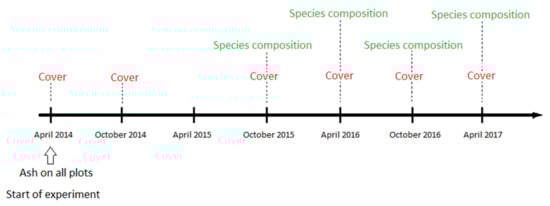
Figure 1.
Timeline for a field experiment where bryophytes on a Norway spruce forest floor treated with wood ash were monitored over a period of three years. At experimental onset in April 2014, we applied six levels of ash to 2 m x 2 m plots, with five replicates of each treatment, i.e., 30 plots in total. Image analysis of bryophyte cover was performed in April 2014, October 2014, October 2015, April 2015, October 2016, and April 2017. Pinpoint registration of species composition was performed in October 2015, April 2016, October 2016, and April 2017.
2.3. Species Composition: Pinpoint Analysis
We used pinpoint analysis to determine the species composition in the 30 plots 1.5, 2, 2.5, and 3 years after ash application (October 2015, April 2016, October 2016, and April 2017). We applied pinpoints for every 20 cm, 11 pinpoints per row in 11 columns; i.e., a total of 121 pinpoints covering the plot completely (Supplementary Materials Figure S2). For each of the 121 pinpoints in each of the 30 plots, we recorded all bryophyte (i.e., mosses and liverworts) species and bare soil; hence, one pinpoint might result in several registrations depending on the number of species underneath it.
2.4. Soil pH vs. Ellenberg Reaction Values
In October 2016, 2.5 years after ash application, we collected three soil cores (diameter 6 cm, depth 3 cm) from each of the 30 plots to measure pH in the top organic layer. We removed the living moss, and used material from the top 1 cm of the remaining soil core. We measured pH (H2O) on a pH meter 240 (Radiometer Copenhagen). Concomitantly, we calculated the Ellenberg Reaction values weighted by abundance, i.e., for each plot, for each particular species, we multiplied its frequency with the Ellenberg values given by [21].
3. Results
3.1. Soil pH and Ellenberg Reaction Values
The soil pH increased with increasing wood ash doses in an asymptotic fashion up to a value of about 8 (Figure 2A). Weighted Ellenberg reaction values for the bryophytes, 2.5 years after ash application, correlated significantly with pH, but with a much steeper slope for the high (15–90 t ha−1) than for the low (0–9 t ha−1) ash doses (Figure 2B).
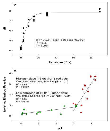
Figure 2.
(A) Correlation between wood ash dose and soil pH 2.5 years after ash application in 30 plots treated with six different levels of ash. Soil pH values are based on mean values for three samples in each of the 30 plots. (B) The relationship between pH and weighted Ellenberg reaction (R) values 2.5 years after ash application. We used Ellenberg values from Hill et al. (2007) and calculated the weighted Ellenberg reaction value in each plot by multiplying the Ellenberg reaction value with the species frequencies in each plot. We divided the values into two groups, those corresponding to the low ash doses (0–9 t ha−1) and those corresponding to the high ash doses (15–90 t ha−1). In both cases, simple linear models showed a positive correlation between pH and Ellenberg reaction (R) values, but for the higher values, the slope was steeper, which suggest that direct ash effect was more prominent than the pH shift.
3.2. Total Bryophyte Cover: Image Analysis
In April 2014, before the ash was applied, the bryophyte cover did not differ significantly between plot types (p = 0.997) with an average cover of (64.6% +/− 1.7, mean +/− SE) (Figure 3, Supplementary Table S2). The effect of ash was most pronounced six months after ash application, here 90 t ash ha−1 reduced the total bryophyte cover to c. 5% compared to c. 90% in the 0 t ha−1 treatment (Figure 3, October 2014). This corresponds to 93.9% decrease in cover. At the following analyses, the cover had started to re-establish, and amounted to 54.3%, 55.5%, 45.8%, and 36.8% reductions, 1.5, 2, 2.5, and 3 years after application of 90 t ash ha−1, respectively (Supplementary Table S2). We observed a higher amount of dead bryophytes six months after application of 3 t ash ha−1 compared to 12 months after ash application while we observed almost no dead bryophytes 18 months after application of 3 and 9 t ash ha−1 (data not shown). Still, all analyses, 0.5–3 years after ash application showed significant correlations between bryophyte cover and ash application (Figure 3, Supplementary Table S2). We notice that apparently bryophyte cover varied between years independently of ash application, and in particular between seasons. Thus, the cover in the 0 t ha−1 plots was significantly lower in spring (April, 0, 2, and 3 years after ash application) compared to autumn (October 0.5, 1.5, and 2.5 years after ash application) (one way ANOVA, p = 0.013).
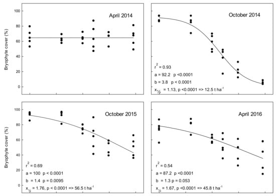
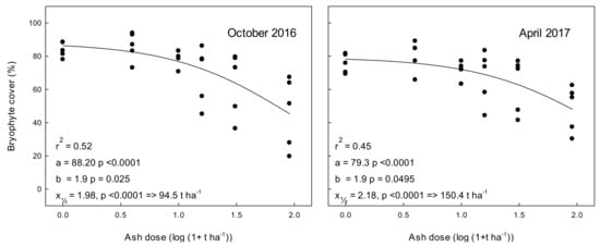
Figure 3.
Total bryophyte cover (%) in experimental 2 m × 2 m plots treated with different levels of wood ash in April 2014 and subsequently evaluated by photo image analysis. Ash doses corresponded to application of 0–90 t ha−1. Note that, in addition to the strong negative relation between ash application and bryophyte cover, moss cover was significantly more developed in autumn than in spring. Time 0 (April 2014) corresponds to bryophyte cover prior to ash application. Dots represent individual measurements and the solid lines show data modelled by the simple three-parameter logistic equation y = a [1 + exp(b(x − x½))]−1 often used for dose response relationships [22]. Here, “a” is the cover in untreated plots (as suggested by the model), “b” indicates how strongly bryophyte cover decreases with ash dose, and “x½“is the value suggested by the model that reduces cover by 50%. Thus, the ash dose predicted by the model to reduce cover by 50% will be 10x½ + 1.
3.3. Species Composition: Pinpoint Analysis
We registered in total 28 moss species and three liverwort species in the sample area, 22 moss species and two liverwort species were recorded in the pinpoint analyses of the 30 plots (Table 2). Some bryophyte species dominated entire plots while others were only found a couple of times. A few species were not recorded at every sampling. The species composition changed gradually with increasing ash application, whereas total species number remained almost constant for the different treatments, with a slight tendency for increased species number at intermediate ash levels. (Figure 4). Although some species were significantly affected by ash dose, species composition differed only slightly between the four sampling times, and time and interaction between time and ash dose had no significant effect (Table 3). Plots without ash were dominated by H. jutlandicum, D. scoparium and P. schreberi, whereas F. hygrometrica, C. purpureus, and B. rutabulum dominated in the 90 t ash ha−1 treatments. H. jutlandicum decreased when ash was applied (Figure 4). The abundance of D. scoparium and L. bidentata also decreased with increasing ash application from doses higher than 3 t ha−1. By contrast, F. hygrometrica and C. purpureus were absent in the 0 t ha−1 plots but increased in abundance with increasing ash application. P. schreberi was present in all treatments, but with the highest abundance in plots treated with 3–15 t ash ha−1. B. rutabulum was most abundant in treatments with 9–90 t ash ha−1.
Table 2.
List of mosses and liverworts recorded during a three-year period in 2 m × 2 m plots treated with wood ash in doses corresponding to 0, 3, 9, 15, 30, and 90 t ha−1. Species marked with an asterisk (*) were registered in the sample area but not recorded in the pinpoint analyses.
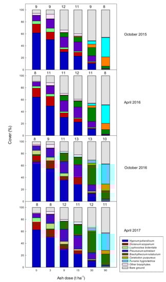
Figure 4.
Cover of the seven most abundant bryophytes and a compound group with the remaining species after treatment with 0, 3, 9, 15, 30, and 90 t ash ha−1. The analyses were made 1.5 (October 2015), 2.0 (April 2016), 2.5 (October 2016), and 3.0 (April 2017) years after ash application. The cover of each species was obtained using a pinpoint analysis with 121 pinpoints covering the 2 m × 2 m plots. For each pinpoint we recorded all bryophyte species. Numbers above the columns indicate how many species occurred in the particular treatments.
Table 3.
ANOVA table presenting F and p values from two-way analysis of variance (time, ash dose and their interaction), of number of observations of the seven most abundant species, other bryophytes and bare soil from pinpoint analyses. Ash dose (t ha−1) and time after ash application (months) were considered quantitative variables. “Model” indicates the complete model (number of observation = time + ash dose + time *ash dose) and “Ash dose” indicates the relationship between observation and ash dose. The number of observations for each species were log(1 + obs.) transformed. Time and time*ash dose were not significant for any of the tested species/parameters and are not included.
4. Discussion
4.1. Investigation of Harmful Effects on Bryophytes in the Field
We used two different methods to assess the ash effect on the bryophytes, (1) photos taken of the plots and subsequent image analysis to measure total cover of bryophytes and (2) in situ pinpoint analysis to obtain detailed information on the species composition. Each of these two methods has advantages and drawbacks.
The image analysis method makes it possible to obtain data in a relatively easy manner, also for persons without detailed knowledge on bryophyte identification. Thus, we could analyse the bryophyte community from early on in the project. Moreover, the method is quick and images gained in the field can be stored for later analysis. This is a great advantage, especially in long-term studies, compared to direct estimation of cover in the field. Total bryophyte cover is often estimated by eye [9,11,12]. This method however, is highly subjective, and often difficult, especially for large plots with a patchy cover.
Pinpoint analysis yields more thorough knowledge of the bryophyte response than the image analysis, as it provides estimates of total cover as well as the cover of each particular species. However, it requires specialist knowledge and experience regarding bryophyte identification, therefore we were unable to perform this analysis at the first time points. In particular, measurements before ash application would have been desirable. However, we consider this less important as the control plots were rather similar and changed little with time. Even though pinpoint analysis is very time-consuming, it yields more exact results, than semi-quantitative evaluation of individual bryophyte species cover by eye [9,10,11], and it increases the chance of recording small species covered by larger species.
The combination of image analysis of total cover and analysis of species composition provides a more complete picture of the moss cover than the two methods would do alone. The pinpoint analysis of species composition is a necessity in more thorough investigations, and in principle it also estimates the total cover. This is, however, less precise as the number of data points reflects the number of pinpoints, while the analysis of total cover in ImageJ depends on the number of pixels in the photo, which is much larger than the number of pinpoints. We observed a large change in species composition especially in plots treated with 30 t and 90 t ash ha−1, with new species appearing. This aspect could not be covered with the image analysis.
4.2. Ash Effects on Bryophytes
The ash effects on bryophytes fall into two categories. The first is the immediate, direct effect on the bryophyte shoots exposed to ash. This effect, caused by the strongly alkaline and osmotic properties of the ash, is described as visible damage or “burning” of bryophytes [9]. The second response is the long-term effect on species composition caused by a change in the physicochemical environment.
Depending on the ash dose, immediate ash effects include discoloration or death of the bryophyte shoots. We observed burning effects on bryophytes after ash application in all ash treatments, which resulted in lower cover and the effect increased with increasing ash doses (Figure 3). At small ash doses the visible damage was mainly discoloration, and the shoots recover within a few months to five years depending on the ash dose and type of ash [9,11,13]. The differences in the total moss cover’s response to ash in different studies also reflect the differences in species composition in the studied forests, as different species respond differently to wood ash (as discussed below).
A limited period of discoloration followed by no visible damage may seem a non-harmful effect, but Kellner and Weibull [11] found a decrease in photosynthetic activity with increasing degree of visible damage. They found similar burning effects caused by liming. Three years after liming, the shoots had fully recovered from visible damage, but Dicranum polysetum still produced a reduced number of sporophytes. This decreased fertility could affect the long-term persistence of a species, especially if large areas are treated.
The pinpoint analyses demonstrated a change in bryophyte species composition after wood ash application (Figure 4). Most prominent was the decrease in Hypnum jutlandicum with increasing ash dose and the appearance and dominance of Brachythecium rutabulum, Ceratodon purpureus, and Funaria hygrometrica at high doses. The total cover of bryophytes in the plots treated with high ash doses (9–90 t ha−1) increased from the analysis 6 months after ash application to the subsequent analyses (Figure 3). This reestablishment of bryophyte cover is partly due to recovery of initial species and partly due to emergence of new species, with the new species being the main source of cover recovery at 30 and 90 t ha−1 (Figure 4).
It is obvious that the different bryophyte species respond differently to ash application, with some species decreasing with increasing ash dose (H. jutlandicum, Dicranum scoparium, Lophocolea bidentata), some increasing with increasing ash dose (C. purpureus, F. hygrometrica), and some having optimum at intermediate ash doses (Pleurozium schreberi, B. rutabulum) (Figure 4). Former studies also report a difference in response to ash for different bryophyte species. This difference is mainly reported as D. polysetum being more susceptible to ash than P. schreberi [9,11]. Equivalent to our study, Silfverberg [23] observed an appearance of F. hygrometrica after application of ash (5 t ha−1), while it was not present in control plots.
The exact wood ash dose that causes increase/decrease in different species varies between studies. This difference is most likely explained by the different properties of ashes due to differences in wood type, combustion and physical form, which result in difference in pH, neutral salts, nutrient composition and concentration, and the rate of release of the chemical components in the ash to the soil [13,24,25]. Further, differences in properties of the specific soil may also influence the bryophyte response.
4.3. pH
In line with Dynesius [14], we found that the bryophyte response to wood ash application related to their pH ecology, i.e., their Ellenberg R-values (Figure 2B). Duliere et al. [15] showed that lime application (5 t ha−1) to Pine and Oak stands both reduced the bryophyte cover and changed the bryophyte species composition. Dicranaceae (Campylopus flexuosus, Dicranum montanum, and Dicranella heteromalla) declined and B. rutabulum, C. purpureus, and F. hygrometrica emerged or expanded. These changes are in line with our finding of bryophyte response to ash application. Thus, increased soil pH is probably an important reason for the change in species composition after ash application with an overall shift in bryophyte community from dominance of acidophilic to alkaliphilic species after ash application.
However, this was more apparent for the higher ash levels (15–90 t ash ha−1). For the lower, 0–9 t ha−1, the effect was slighter, despite the soil pH increase already at 3 t ha−1 (Figure 2A), which illustrates that the combination of pH effects and the immediate “burning” paves the way for the ephemeral species with higher Ellenberg-R values. At intermediate ash levels, (3–15 t ha−1) Hypnum jutlandicum was replaced by Pleurozium schreberi (Figure 4), which both have Ellenberg R values of 2 [21]. Thus, the species list provides a more detailed picture than the Ellenberg values alone. The weighted Ellenberg R value increased conspicuously when Brachythecium rutabulum, Ceratodon purpureus, and Funaria hygrometrica became abundant in the plots, as these species have high Ellenberg reaction values (6, 5, and 6, respectively).
4.4. Nutrients
Wood ash contains the essential plant nutrients (Table 1 and [2]), except nitrogen. However, wood ash stimulates microbial activity, which also increases soil nitrogen availability [7]. Ozolinčius et al. [10] measured the concentration of nutrients in Pleurozium schreberi, and found a significant increase in P, Ca and Mg two years after application of 5 t ash ha−1. The increase in nutrients will affect different species differently, as some bryophytes (just like tracheophytes) are adapted to nutrient rich conditions while others are adapted to nutrient poor habitats. This is reflected in their Ellenberg-N values, which is a general indicator of fertility [21]. Considering their response to ash application, P. schreberi and C. purpureus have remarkably low Ellenberg N values (2 and 3, respectively), which again illustrates that these values do not provide the full picture. The Ellenberg N values for H. jutlandicum, D. scoparium, D. polysetum, B. rutabulum, and F. hygrometrica (2, 2, 2, 6, and 7, respectively) correspond to their response to the increase in nutrients due to ash application.
4.5. Reestablishment and Succession of Bryophytes after Ash Application
Treatment with wood ash resembles fire in terms of removal of vegetation, increase in mineral nutrients and other metal ions and increase in pH. For example, Paquette et al. [24] found a decreased cover of perennial bryophyte species and increased cover of ephemeral colonists after forest fires. Likewise, Calabria et al. [26] found a greater biomass of colonist mosses after fires on prairies, while the biomass of all other functional groups of bryophytes decreased. Further, Rees and Juday [27] reported an almost complete shift in bryophyte species composition from early successional stages (c. 10 years after fire) to later stages (c. 40 years after fire). This shift in species composition was also observed by Rydgren et al. [28] after removal of the vegetation and top soil. They predicted that the reestablishment of the pre-disturbance community would take up to 30 years.
The increased soil pH after wood ash application may prevail for many years. Saarsalmi et al. [29] found a higher soil pH even 16 years after application of 3 t ash ha−1. As pH is a major driver of the changes in species composition following ash application, reestablishment of the initial species composition may be slow. Furthermore, in forestry, application of ash as fertilizer will be repeated up to three applications of 3 t ha−1 during 75 years [3]. Hence, the soil pH is likely to increase further with every ash application. Thus, a more alkaliphilic bryophyte community will establish in plantations treated with ash. The shift in bryophyte species composition after application of especially high doses of ash may be explained by successional patterns as well as pH-ecology. When the ground vegetation has been cleared by the ash, small opportunistic colonisers, e.g., the acrocarpous C. purpureus and F. hygrometrica get a chance to establish.
4.6. Effects on Diversity and Ecosystem Services
At the currently allowed maximum dose for wood ash application in Danish forests of 3 t ash ha−1, and overall similar recommendations in Sweden, Finland, and Lithuania [4], we found only minor changes in total bryophyte cover compared to the untreated plots, when assessed 0.5−3 years after ash application (Figure 3). The composition of the bryophyte community, though, was more susceptible to even small doses of ash and changed, resulting in a lower abundance of H. jutlandicum and a higher abundance of P. schreberi (Figure 4, Table 3). At ash doses ≥30 t ha−1, we observed a complete change in bryophyte composition, where F. hygrometrica, C. purpureus, and B. rutabulum dominated the plots.
The vegetation in production plantations in Central Jutland is usually not associated with high conservation value. Still, we found one species in our experimental area, Dicranum spurium, which is categorised as Vulnerable (VU) in the Danish Red List [30], though it occurred in low numbers and was not registered in the pinpoint analyses (Table 2). D. spurium normally occurs in heathland and is presently known from less than 10 locations in Denmark. It prefers acidic conditions with an Ellenberg reaction value of 2 [21]. Thus, extensive wood ash application will most likely eliminate this, and possibly other, vulnerable species.
The dominating species in the plots without ash (H. jutlandicum, P. schreberi, and D. scoparium) make dense carpets (H. jutlandicum and P. schreberi) and/or are up to 15 cm tall (P. schreberi and D. scoparium), resulting in a thick continuous and persistent moss layer covering the ground. F. hygrometrica and C. purpureus on the other hand are small and slender acrocarps that barely cover the ground and do not grow taller than a couple of cm. A huge number of different invertebrates, collembolans, mites, earthworms, spiders etc. that inhabit the bryosphere [25], will be affected by the change in species composition. Furthermore, the thick bryophyte layer insulates the soil and retains humidity. Even at relatively low ash applications (≤9 t ha−1), we observed a larger abundance of B. rutabulum, which forms flatter and loser carpets, and thus makes up a poorer habitat for moss dwellers. Still, if ash is only applied in plantations with regular clear-cuts and where especially slash harvest affects the bryophytes [31,32], application of even relatively high (e.g., 9 t ha−1 or 15 t ha−1) ash doses will have minor effects compared to these radical actions.
Finally, the change in bryophyte species composition is a potential problem for commercial harvesting of moss. In Denmark, most of the spruce plantations are on cultivated heathland, where export of moss represents a large proportion of the income. Hypnum jutlandicum is the key species when it comes to export of mosses from Denmark [33], and the application of ash could be a problem in forests used for moss collection.
5. Conclusions
We used two complementary methods, image analysis and pinpoint registration, to study the impact on the bryophyte biota of a wide range of levels of wood ash in a Danish Norway spruce (Picea abies) plantation. To our knowledge, this is the first investigation of such a combined effort, which provides a much more exhaustive description of the effects that if the methods were used separately, and only few levels were tested. We found that the maximum ash dose can be raised above the current legislation limits of 3 t ha−1 to between 3 t ha−1 and 9 t ha−1 without major impacts on the total bryophyte cover. However, even the 3 t ha−1 dose affected species composition, and may likely harm vulnerable species like Dicranum spurium. The change in species composition may also affect the fauna living in the bryosphere. Finally, even application of ash in small doses reduced H. jutlandicum, which is used commercially in some plantations.
Supplementary Materials
The following are available online at https://www.mdpi.com/1999-4907/12/2/178/s1, Figure S1: Measurement of total bryophyte cover, using the program ImageJ. Left: picture of a 2 m × 2 m plot, two years after receiving 15 t ash ha−1. Right: The same picture, where the area outside the plot is cut away and green areas are marked red, by adjusting saturation and hue in the program ImageJ. The percentage of green (red) area is based on the marked pixels, Figure S2: Pinpoint analysis of a plot 1.5 years after receiving 90 t ash ha−1. On each string 11 knots, with a mutual distance of 20 cm, mark the pinpoints. A total of 11 strings covered the plot, with 20 cm between each string. The vegetation was recorded under each of the 121 knots. Registrations included mosses, liverworts, and bare ground. For one pinpoint, several registrations were possible, hence the total number of registrations exceeded 121, Table S1: Vascular plants recorded in the experimental area. No vascular plants were detected by the pinpoint analysis, Table S2: Total cover of bryophytes (%), based on image analysis of photos, before (t = 0), and 0.5, 1.5, 2, 2.5, and 3 years after ash application. Mean values, standard errors in brackets. N = 5. Values followed by similar letters do not differ significantly (one way ANOVA on the particular years, Tukey two-way comparison).
Author Contributions
All authors contributed to planning, processing of data, and writing. All authors have read and agreed to the published version of the manuscript.
Funding
The research formed part of Center for Energy Recycling, ASHBACK, funded by the Danish Council of Strategic Research (DSF-12-132655). RR and FE were funded by Danish Council for Independent Research (DFF-4002-00274 and 9040-00314B).
Data Availability Statement
Data available on request due to restrictions eg privacy or ethical.
Acknowledgments
We sincerely thank Ditte Frydensberg and Jeppe Ethelberg-Findsen who assisted during the field work.
Conflicts of Interest
The authors declare no conflict of interest.
References
- Olsson, M.; Rosén, K.; Melkerud, P.-A. Regional modelling of base cation losses from Swedish forest soils due to whole-tree harvesting. Appl. Geochem. 1993, 2, 189–194. [Google Scholar] [CrossRef]
- Pitman, R.M. Wood ash use in forestry—A review of the environmental impacts. Forestry 2006, 79, 563–588. [Google Scholar] [CrossRef]
- Poulsen, T.L. Bekendtgørelse om Anvendelse af Bioaske til Jordbrugsformål (Bioaskebekendtgørelsen). BEK nr 818 af 21/07/2008. 2008. Available online: https://www.retsinformation.dk/eli/lta/2008/818 (accessed on 6 December 2020).
- Karltun, E.; Saarsalmi, A.; Ingerslev, M.; Mandre, M.; Andersson, S.; Gaitnieks, T.; Ozolinčius, R.; Varnagiryte-Kabasinskiene, I. Wood Ash Recycling-Possibilities and Risks. In Sustainable Use of Forest Biomass for Energy; Managing Forest Ecosystems; Röser, D., Asikainen, A., Raulund-Rasmussen, K., Stupak, I., Eds.; Springer: Dordrecht, The Netherlands, 2008; Volume 12, pp. 79–108. [Google Scholar]
- Jean, M.; Alexander, H.D.; Mack, M.C.; Johnstone, J.F. Patterns of bryophyte succession in a 160-year chronosequence in deciduous and coniferous forests of boreal Alaska. Can. J. For. Res. 2017, 47, 1021–1032. [Google Scholar] [CrossRef]
- Kindtler, N.L.; Ekelund, F.; Rønn, R.; Kjøller, R.; Hovmand, M.F.; Madsen, M.V.; Christensen, S.; Johansen, J.L. Wood ash effects on growth and cadmium uptake in Deschampsia flexuosa (Wavy hair-grass). Environ. Pollut. 2019, 249, 886–893. [Google Scholar] [CrossRef] [PubMed]
- Vestergård, M.; Bang-Andreasen, T.; Buss, S.B.; Cruz-Paredes, C.; Bentzon-Tilia, S.; Ekelund, F.; Kjøller, R.; Mortensen, L.H.; Rønn, R. The relative importance of the bacterial pathway and soil inorganic nitrogen increase across an extreme wood ash application gradient. Glob. Chang. Biol. Bioenergy 2018, 10, 320–334. [Google Scholar] [CrossRef]
- Bang-Andreasen, T.; Nielsen, J.T.; Voriskova, J.; Heise, J.; Rønn, R.; Kjøller, R.; Bruun Hansen, H.C.; Jacobsen, C.S. Wood ash induced pH changes strongly affect soil bacterial numbers and community composition. Front. Microbiol. 2017, 8, 1400. [Google Scholar] [CrossRef]
- Jacobson, S.; Gustafsson, L. Effects on ground vegetation of the aplication of wood ash to a Swedish Scots pine stand. Basic Appl. Ecol. 2001, 2, 223–241. [Google Scholar] [CrossRef]
- Ozolinčius, R.; Buožyte, R.; Varnagiryte-Kabašinskiene, I. Wood ash and nitrogen influence on ground vegetation cover and chemical composition. Biomass Bioenergy 2007, 31, 710–716. [Google Scholar] [CrossRef]
- Kellner, O.; Weibull, H. Effects of Wood Ash on Bryophytes and Lichens in a Swedish Pine Forest.pdf. Scand. J. For. Res. 1998, 2, 76–85. [Google Scholar]
- Arvidsson, H.; Vestin, T.; Lundkvist, H. Effects of crushed wood ash on soil chemistry in young Norway spruce stands. For. Ecol. Manag. 2002, 161, 75–87. [Google Scholar] [CrossRef]
- Skov, S.; Ingerslev, M. Biologisk Respons på Flisaske i Skove; Institut for Geovidenskab og Naturforvaltning, Københavns Universitet: Frederiksberg, Denmark, 2014. [Google Scholar]
- Dynesius, M. Responses of bryophytes to wood-ash recycling are related to their phylogeny and pH ecology. Perspect. Plant Ecol. Evol. Syst. 2012, 14, 21–31. [Google Scholar] [CrossRef]
- Duliere, J.F.; Carnol, M.; Dalem, S.; Remacle, J.; Malaisse, F. Impact of dolomite lime on the ground vegetation and on potential net N transformations in Norway spruce (Picea abies (L.) Karst.) and sessile oak (Quercus petraea (Matt.) Lieb.) stands in the Belgian Ardenne. Ann. For. Sci. 1999, 56, 361–370. [Google Scholar] [CrossRef]
- Jäppinen, J.P.; Hotanen, J.P. Effect of fertilization on the abundance of bryophytes in two drained peatland forests in Eastern Finland. Ann. Bot. Fenn. 1990, 27, 93–108. [Google Scholar]
- Yang, W.; Magid, J.; Christensen, S.; Rønn, R.; Ambus, P.; Ekelund, F. Biological fractionation of 13C increases with increasing biodiversity. Soil Biol. Biochem. 2014, 69, 197–201. [Google Scholar] [CrossRef]
- Hansen, M.; Kepfer-Rojas, S.; Bjerager, P.E.R.; Holm, P.E.; Skov, S.; Ingerslev, M. Effects of ash application on nutrient and heavy metal fluxes in the soil and soil solution in a Norway spruce plantation in Denmark. For. Ecol. Manag. 2018, 424, 494–504. [Google Scholar] [CrossRef]
- Wang, P.R. Klimagrid Danmark- Referenceværdier 2001–2010; Teknisk Rapport 13-09; Danmarks Meterologiske Institut, Klima- og Energiministeriet: København, Danmark, 2013. [Google Scholar]
- Maresca, A.; Hansen, M.; Ingerslev, M.; Astrup, T.F. Column leaching from a Danish forest soil amended with wood ashes: Fate of major and trace elements. Biomass Bioenergy 2018, 109, 91–99. [Google Scholar] [CrossRef]
- Hill, M.O.; Preston, C.D.; Bosanquet, S.D.S.; Roy, D.B. BRYOATT. In Attributes of British and Irish Mosses, Liverworts and Hornworts; NERC Centre for Ecology and Hydrology and Countryside Council for Wales: Huntingdon, UK, 2007. [Google Scholar]
- Johansen, J.L.; Rønn, R.; Ekelund, F. Toxicity of cadmium and zinc to small soil protists. Environ. Pollut. 2018, 242, 1510–1517. [Google Scholar] [CrossRef]
- Silfverberg, K. Forest regeneration on nutrient-poor peatlands: Effects of fertilization, mounding and sowing. Silva Fennica 1995, 29, 205–215. [Google Scholar] [CrossRef][Green Version]
- Paquette, M.; Boudreault, C.; Fenton, N.; Pothier, D.; Bergeron, Y. Bryophyte species assemblages in fire and clear-cut origin boreal forests. Forest Ecol. Manag. 2016, 359, 99–108. [Google Scholar] [CrossRef]
- Glime, J.M. Bryophyte Ecology, Volume 2: Bryological Interaction. 2017. Available online: https://digitalcommons.mtu.edu/bryophyte-ecology2/ (accessed on 5 August 2020).
- Calabria, L.M.; Petersen, K.; Hamman, S.T.; Smith, R.J. Prescribed Fire Decreases Lichen and Bryophyte Biomass and Alters Functional Group Composition in Pacific Northwest Prairies. Northwest Sci. 2016, 90, 470–483. [Google Scholar] [CrossRef]
- Rees, D.C.; Juday, G.P. Plant species diversity and forest structure on logged and burned sites in central Alaska. For. Ecol. Manag. 2002, 155, 291–302. [Google Scholar] [CrossRef]
- Rydgren, A.K.; Økland, R.H.; Hestmark, G. Disturbance Severity and Community Resilience in a Boreal Forest. Ecology 2004, 85, 1906–1915. [Google Scholar] [CrossRef]
- Saarsalmi, A.; Mälkönen, E.; Piirainen, S. Effects of Wood Ash Fertilization on Forest Soil Chemical Properties. Silva Fennica 2001, 35, 355–368. [Google Scholar] [CrossRef]
- Goldberg, I. Mosser. In The Danish Red list (Den danske Rødliste in Danish) 2019; Moeslund, J.E., Nygaard, B., Ejrnæs, R., Bell, N., Bruun, L.D., Bygebjerg, R., Carl, H., Damgaard, J., Dylmer, E., Elmeros, M., et al., Eds.; Aarhus Universitet: Aarhus, Denmark, 2019; Available online: https://bios.au.dk/forskningraadgivning/temasider/redlistframe/artsgrupperne/planter/mosser/ (accessed on 24 July 2020).
- Åström, M.; Dynesius, M.; Hylander, K.; Nilsson, C. Effects of slash harvest on bryophytes and vascular plants in southern boreal forest clear-cuts. J. Appl. Ecol. 2005, 42, 1194–1202. [Google Scholar] [CrossRef]
- Dynesius, M.; Astrom, M.; Nilsson, C. Microclimatic buffering by logging residues and forest edges reduces clear-cutting impacts on forest bryophytes. Appl. Veg. Sci. 2008, 11, 345–354. [Google Scholar] [CrossRef]
- Hansen, H.; (“JYSK MOS APS”, Brande, Denmark). Personal communication, 2019.


Publisher’s Note: MDPI stays neutral with regard to jurisdictional claims in published maps and institutional affiliations. |
© 2021 by the authors. Licensee MDPI, Basel, Switzerland. This article is an open access article distributed under the terms and conditions of the Creative Commons Attribution (CC BY) license (http://creativecommons.org/licenses/by/4.0/).