
Exploring the Potential Distribution of Relic Trochodendron aralioides: An Approach Using Open-Access Resources and Free Software


Abstract
:
1. Introduction
2. Materials and Methods
2.1. Target Species
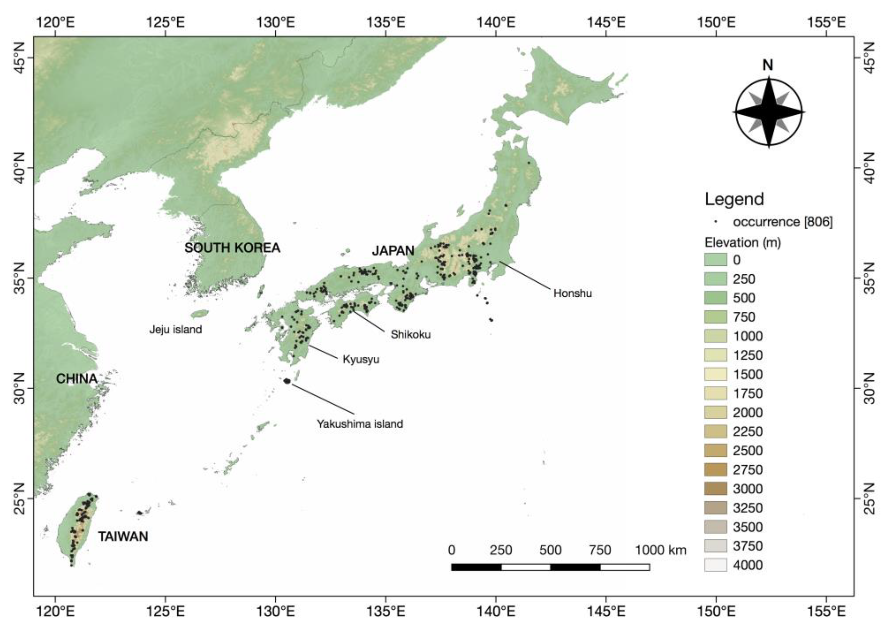
2.2. Target Area
2.3. Open-Access Resources and Free Software
2.3.1. Species Occurrences
2.3.2. Environmental Variables
2.3.3. GIS: GRASS GIS and QGIS
2.3.4. MaxEnt
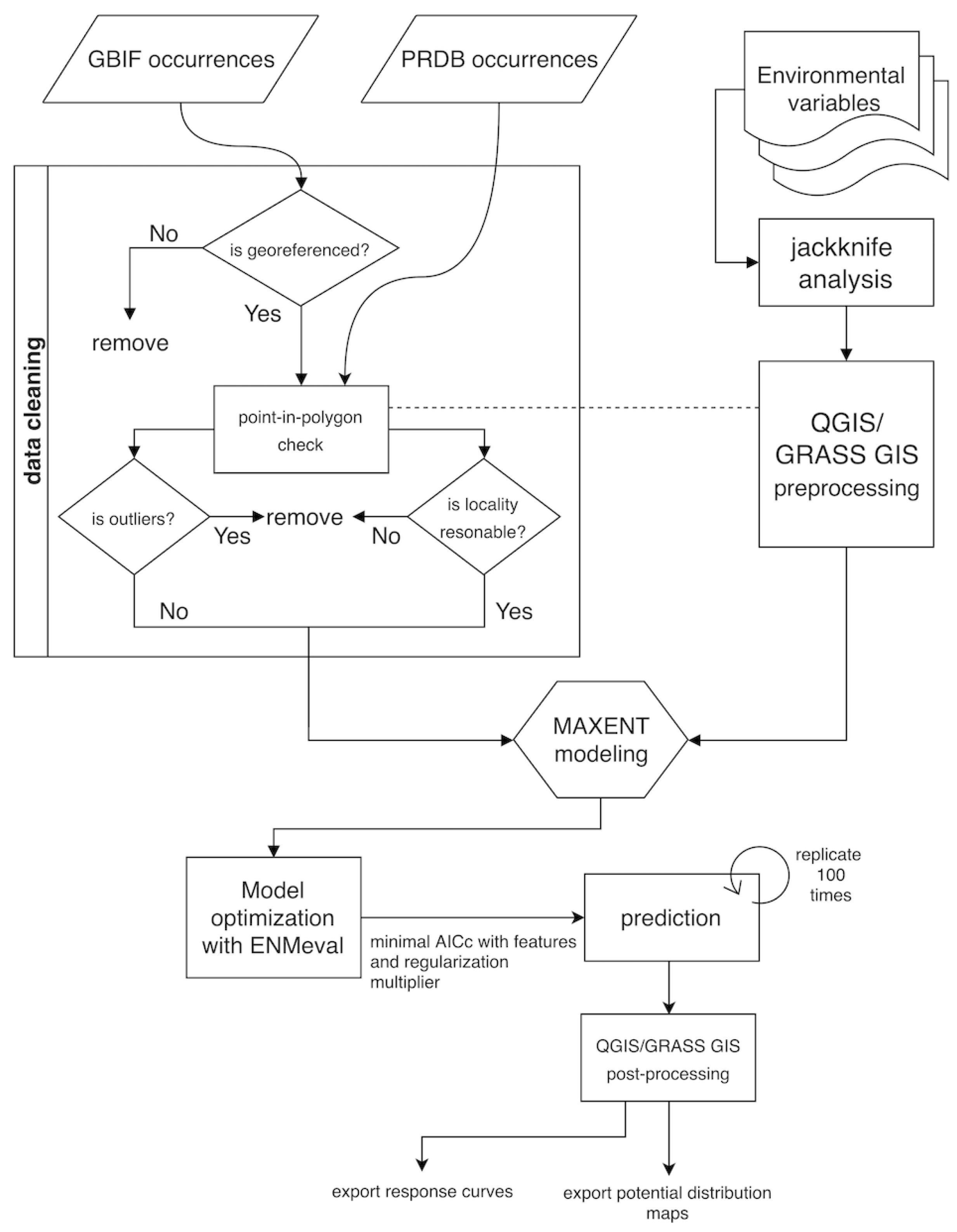
2.4. Model Building and Validation
3. Results
3.1. Species Dataset
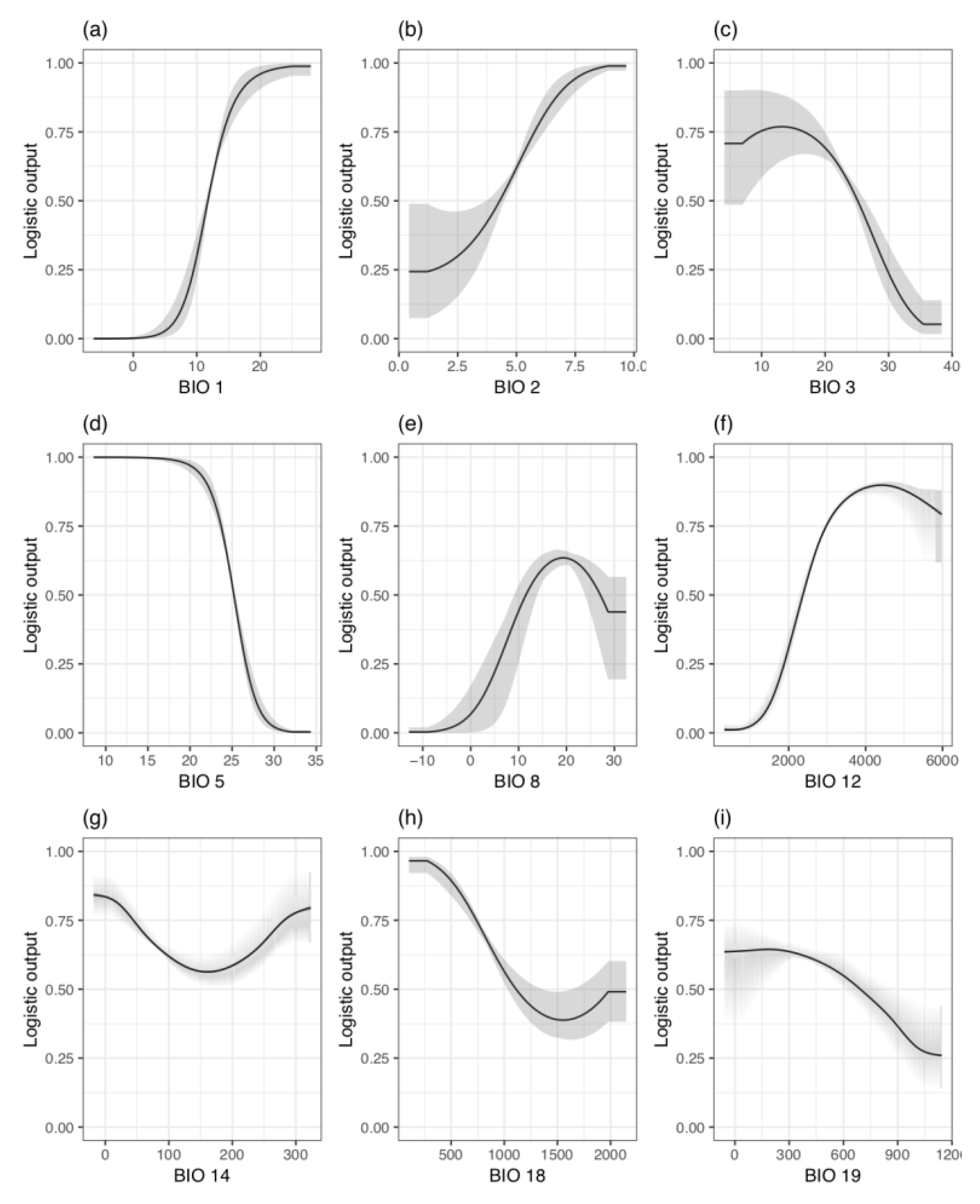
3.2. MaxEnt Modeling and Performance
4. Discussion
4.1. Data Quality for Species Occurrence
4.2. Distribution of T. aralioides
4.2.1. Japan
4.2.2. Taiwan
4.3. T. aralioides in South Korea?
5. Conclusions
Supplementary Materials
Author Contributions
Funding
Institutional Review Board Statement
Informed Consent Statement
Data Availability Statement
Conflicts of Interest
References
- Fu, D.; Endress, P. Trochodendraceae. In Flora of China; Wu, Z., Ed.; Science Press: Beijing, China; St. Louis, MI, USA, 2001; Volume 6, p. 124. [Google Scholar]
- Stevens, P.F.; Angiosperm Phylogeny Website. Version 12. Available online: http://www.mobot.org/MOBOT/research/APweb/ (accessed on 19 September 2021).
- Lu, A.-M.; Li, J.-Q.; Chen, Z.-D. The origin and dispersal of the “lower” Hamamelidae. J. Syst. Evol. 1993, 31, 489–504. [Google Scholar]
- Manchester, S.R.; Crane, P.R.; Dilcher, D.L. Nordenskioldia and Trochodendron (Trochodendraceae) from the Miocene of Northwestern North America. Bot. Gaz. 1991, 152, 357–368. [Google Scholar] [CrossRef]
- Pigg, K.B.; Wehr, W.C.; Ickert-Bond, S.M. Trochodendron and Nordenskioldia (Trochodendraceae) from the Middle Eocene of Washington State, U.S.A. Int. J. Plant Sci. 2001, 162, 1187–1198. [Google Scholar] [CrossRef] [Green Version]
- Pigg, K.B.; Dillhoff, R.M.; DeVore, M.L.; Wehr, W.C. New diversity among the Trochodendraceae from the early/middle Eocene Okanogan Highlands of British Columbia, Canada, and northeastern Washington State, United States. Int. J. Plant Sci. 2007, 168, 521–532. [Google Scholar] [CrossRef] [Green Version]
- Li, H.; Chaw, S. Trochodendraceae. In Flora of Taiwan; Editorial Committee of Flora of Taiwan, Ed.; National Taiwan University: Taipei, Taiwan, 1996; Volume 2, pp. 504–505. [Google Scholar]
- Su, H.-J. Studies on the climate and vegetation types of the natural forest in Taiwan. (II). Altitudinal vegetation zones in relation to temperature gradient. QJ Chin. For. 1984, 17, 57–73. [Google Scholar]
- Yahara, T. Phytogeographical problems in the temperate flora in Japan. Current aspect of biogeography in west Pacific and East Asian regions. In Current Aspects of Biogeography in West Pacific and East Asian Regions; Oba, H., Hayami, I., Mochizuki, K., Eds.; University Museum, University of Tokyo, Nature and Culture: Tokyo, Japan, 1989; pp. 99–114. [Google Scholar]
- Cronquist, A. An Integrated System of Classification of Flowering Plants; Columbia University Press: New York, NY, USA, 1981; ISBN 9780231038805. [Google Scholar]
- Mabberley, D.J. The Plant-Book: A Portable Dictionary of the Higher Plants; Cambridge University Press: Cambridge, UK, 1997; ISBN 0524414210. [Google Scholar]
- Hatushima, S. Flora of the Ryukyus: (Including Amami Islands, Okinawa Islands, and Sakishima Archipelago); Okinawa Society of Biological Education and Research: Okinawa, Japan, 1971. (In Japanese) [Google Scholar]
- Wu, J.-E.; Huang, S.; Wang, J.-C.; Tong, W.-F. Allozyme variation and the genetic structure of populations of Trochodendron aralioides, a monotypic and narrow geographic genus. J. Plant Res. 2001, 114, 45–57. [Google Scholar] [CrossRef]
- Andrews, S. Tree of the Year: Trochodendron aralioides; International Dendrology Society: Herefordshire, UK, 2009; p. 48. [Google Scholar]
- Wu, H.; Su, H.; Hu, J. The identification of A-, B-, C-, and E-Class MADS-box genes and implications for perianth evolution in the basal eudicot Trochodendron aralioides (Trochodendraceae). Int. J. Plant Sci. 2007, 168, 775–799. [Google Scholar] [CrossRef] [Green Version]
- Yang, X.; Lu, S.; Peng, H. Cytological studies on the eastern Asian family Trochodendraceae. Bot. J. Linn. Soc. 2008, 158, 332–335. [Google Scholar] [CrossRef]
- Ohwi, J. Trochodendraceae. In Flora of Japan; Meyer, F., Walker, E., Eds.; Smithsonian Institution: Washington, DC, USA, 1965; p. 438. [Google Scholar]
- Austin, M.P. Spatial prediction of species distribution: An interface between ecological theory and statistical modelling. Ecol. Model. 2002, 157, 101–118. [Google Scholar] [CrossRef] [Green Version]
- Elith, J.; Leathwick, J.R. Species distribution models: Ecological explanation and prediction across space and time. Annu. Rev. Ecol. Evol. Syst. 2009, 40, 677–697. [Google Scholar] [CrossRef]
- Guisan, A.; Thuiller, W. Predicting species distribution: Offering more than simple habitat models. Ecol. Lett. 2005, 8, 993–1009. [Google Scholar] [CrossRef]
- Guisan, A.; Zimmermann, N.E. Predictive habitat distribution models in ecology. Ecol. Model. 2000, 135, 147–186. [Google Scholar] [CrossRef]
- Rodríguez-Castañeda, G.; Hof, A.R.; Jansson, R.; Harding, L.E. Predicting the fate of biodiversity using species’ distribution models: Enhancing model comparability and repeatability. PLoS ONE 2012, 7, e44402. [Google Scholar] [CrossRef] [PubMed] [Green Version]
- Sinclair, S.; White, M.; Newell, G. How useful are species distribution models for managing biodiversity under future climates? Ecol. Soc. 2010, 15, 8. [Google Scholar] [CrossRef]
- Whitehead, A.L.; Kujala, H.; Ives, C.D.; Gordon, A.; Lentini, P.E.; Wintle, B.A.; Nicholson, E.; Raymond, C.M. Integrating biological and social values when prioritizing places for biodiversity conservation. Conserv. Biol. 2014, 28, 992–1003. [Google Scholar] [CrossRef] [PubMed]
- Corsi, F.; Leeuw, J.; de Skidmore, A. Modeling species distribution with GIS. In Research Techniques in Animal Ecology; Boitani, L., Fuller, T., Eds.; Columbia University Press: New York, NY, USA, 2000; pp. 389–434. [Google Scholar]
- Gogol-Prokurat, M. Predicting habitat suitability for rare plants at local spatial scales using a species distribution model. Ecol. Appl. 2011, 21, 33–47. [Google Scholar] [CrossRef]
- Pandit, S.N.; Hayward, A.; Leeuw, J.; de Kolasa, J. Does plot size affect the performance of GIS-based species distribution models? J. Geogr. Syst. 2010, 12, 389–407. [Google Scholar] [CrossRef]
- Fick, S.E.; Hijmans, R.J. WorldClim 2: New 1-km spatial resolution climate surfaces for global land areas. Int. J. Climatol. 2017, 37, 4302–4315. [Google Scholar] [CrossRef]
- Karger, D.N.; Conrad, O.; Böhner, J.; Kawohl, T.; Kreft, H.; Soria-Auza, R.W.; Zimmermann, N.E.; Linder, H.P.; Kessler, M. Climatologies at high resolution for the earth’s land surface areas. Sci. Data 2017, 4, 170122. [Google Scholar] [CrossRef] [Green Version]
- Arzberger, P.; Schroeder, P.; Beaulieu, A.; Bowker, G.; Casey, K.; Laaksonen, L.; Moorman, D.; Uhlir, P.; Wouters, P. Promoting access to public research data for scientific, economic, and social development. Data Sci. J. 2004, 3, 135–152. [Google Scholar] [CrossRef]
- Miller, R.H.; Masuoka, P.; Klein, T.A.; Kim, H.-C.; Somer, T.; Grieco, J. Ecological niche modeling to estimate the distribution of Japanese Encephalitis virus in Asia. PLoS Neglect. Trop. Dis. 2012, 6, e1678. [Google Scholar] [CrossRef] [PubMed] [Green Version]
- Probert, R.J.; Daws, M.I.; Hay, F.R. Ecological correlates of ex situ seed longevity: A comparative study on 195 species. Ann. Bot. 2009, 104, 57–69. [Google Scholar] [CrossRef] [Green Version]
- Tenopir, C.; Allard, S.; Douglass, K.; Aydinoglu, A.U.; Wu, L.; Read, E.; Manoff, M.; Frame, M. Data sharing by scientists: Practices and perceptions. PLoS ONE 2011, 6, e21101. [Google Scholar] [CrossRef] [PubMed] [Green Version]
- Seltzer, C. Making biodiversity data social, shareable, and scalable: Reflections on iNaturalist & citizen science. Biodivers. Inf. Sci. Stand. 2019, 3, e46670. [Google Scholar] [CrossRef]
- Watson, L.; Dallwitz, M.J. The Families of Flowering Plants: Descriptions, Illustrations, Identification, and Information Retrieval. Available online: http://delta-intkey.com/angio (accessed on 25 June 2017).
- Tanaka, N. PRDB (Phytosociological Relevé Data Base). Available online: http://www.ffpri.affrc.go.jp/labs/prdb/EnglishVer/index-e.html (accessed on 23 July 2018).
- Guralnick, R.P.; Hill, A.W.; Lane, M. Towards a collaborative, global infrastructure for biodiversity assessment. Ecol. Lett. 2007, 10, 663–672. [Google Scholar] [CrossRef] [PubMed] [Green Version]
- Porretta, D.; Mastrantonio, V.; Bellini, R.; Somboon, P.; Urbanelli, S. Glacial history of a modern invader: Phylogeography and species distribution modelling of the Asian tiger mosquito Aedes albopictus. PLoS ONE 2012, 7, e44515. [Google Scholar] [CrossRef]
- Chamberlain, S.A.; Boettiger, C. R Python, and Ruby clients for GBIF species occurrence data. PeerJ Prepr. 2017, 5, e3304v1. [Google Scholar] [CrossRef]
- Maletic, J.; Marcus, A. Data cleansing: Beyond integrity analysis. In Proceedings of the 2000 Conference on Information Quality, Cambridge, MA, USA, 25–28 October 2000. [Google Scholar]
- Ashraf, U.; Ali, H.; Chaudry, M.N.; Ashraf, I.; Batool, A.; Saqib, Z. Predicting the potential distribution of Olea ferruginea in Pakistan incorporating climate change by using Maxent model. Sustainability 2016, 8, 722. [Google Scholar] [CrossRef] [Green Version]
- Meneguzzi, V.C.; Dos Santos, C.B.; Leite, G.R.; Fux, B.; Falqueto, A. Niche modelling of Phlebotomine sand flies and Cutaneous leishmaniasis identifies Lutzomyia intermedia as the main vector species in southeastern Brazil. PLoS ONE 2016, 11, e0164580. [Google Scholar] [CrossRef]
- Porto, T.J.; Carnaval, A.C.; Rocha, P.L.B. da Evaluating forest refugial models using species distribution models, model filling and inclusion: A case study with 14 Brazilian species. Divers. Distrib. 2013, 19, 330–340. [Google Scholar] [CrossRef]
- Rupprecht, F.; Oldeland, J.; Finckh, M. Modelling potential distribution of the threatened tree species Juniperus oxycedrus: How to evaluate the predictions of different modelling approaches? J. Veg. Sci. 2011, 22, 647–659. [Google Scholar] [CrossRef]
- Kriticos, D.J.; Webber, B.L.; Leriche, A.; Ota, N.; Macadam, I.; Bathols, J.; Scott, J.K. CliMond: Global high-resolution historical and future scenario climate surfaces for bioclimatic modelling. Methods Ecol. Evol. 2012, 3, 53–64. [Google Scholar] [CrossRef]
- Parra, J.L.; Graham, C.C.; Freile, J.F. Evaluating alternative data sets for ecological niche models of birds in the Andes. Ecography 2004, 27, 350–360. [Google Scholar] [CrossRef]
- Syfert, M.M.; Smith, M.J.; Coomes, D.A. The effects of sampling bias and model complexity on the predictive performance of maxent species distribution models. PLoS ONE 2013, 8, e55158. [Google Scholar] [CrossRef]
- Neteler, M.; Bowman, M.H.; Landa, M.; Metz, M. GRASS GIS: A multi-purpose open source GIS. Environ. Model. Softw. 2012, 31, 124–130. [Google Scholar] [CrossRef] [Green Version]
- Phillips, S.J.; Anderson, R.P.; Schapire, R.E. Maximum entropy modeling of species geographic distributions. Ecol. Model. 2006, 190, 231–259. [Google Scholar] [CrossRef] [Green Version]
- Thuiller, W.; Lafourcade, B.; Engler, R.; Araújo, M.B. BIOMOD—A platform for ensemble forecasting of species distributions. Ecography 2009, 32, 369–373. [Google Scholar] [CrossRef]
- Baldwin, R.A. Use of maximum entropy modeling in wildlife research. Entropy 2009, 11, 854–866. [Google Scholar] [CrossRef]
- Moudrý, V.; Šímová, P. Influence of positional accuracy, sample size and scale on modelling species distributions: A review. Int. J. Geogr. Inf. Sci. 2012, 26, 2083–2095. [Google Scholar] [CrossRef]
- Graham, C.H.; Elith, J.; Hijmans, R.J.; Guisan, A.; Peterson, A.T.; Loiselle, B.A.; The Nceas Predicting Species Distributions Working Group. The influence of spatial errors in species occurrence data used in distribution models. J. Appl. Ecol. 2008, 45, 239–247. [Google Scholar] [CrossRef] [Green Version]
- Hernandez, P.A.; Graham, C.H.; Master, L.L.; Albert, D.L. The effect of sample size and species characteristics on performance of different species distribution modeling methods. Ecography 2006, 29, 773–785. [Google Scholar] [CrossRef]
- Wisz, M.S.; Hijmans, R.J.; Li, J.; Peterson, A.T.; Graham, C.H.; Guisan, A.; Group†, N.P.S.D.W. Effects of sample size on the performance of species distribution models. Divers. Distrib. 2008, 14, 763–773. [Google Scholar] [CrossRef]
- Muscarella, R.; Galante, P.J.; Soley-Guardia, M.; Boria, R.A.; Kass, J.M.; Uriarte, M.; Anderson, R.P. ENMeval: An R package for conducting spatially independent evaluations and estimating optimal model complexity for Maxent ecological niche models. Methods Ecol. Evol. 2014, 5, 1198–1205. [Google Scholar] [CrossRef]
- Warren, D.L.; Seifert, S.N. Ecological niche modeling in Maxent: The importance of model complexity and the performance of model selection criteria. Ecol. Appl. 2011, 21, 335–342. [Google Scholar] [CrossRef] [PubMed] [Green Version]
- Swets, J.A. Measuring the accuracy of diagnostic systems. Science 1988, 240, 1285–1293. [Google Scholar] [CrossRef] [Green Version]
- Lobo, J.M.; Jiménez-Valverde, A.; Real, R. AUC: A misleading measure of the performance of predictive distribution models. Glob. Ecol. Biogeogr. 2008, 17, 145–151. [Google Scholar] [CrossRef]
- Fourcade, Y.; Besnard, A.G.; Secondi, J. Paintings predict the distribution of species, or the challenge of selecting environmental predictors and evaluation statistics. Glob. Ecol. Biogeogr. 2018, 27, 245–256. [Google Scholar] [CrossRef]
- Daru, B.H.; Park, D.S.; Primack, R.B.; Willis, C.G.; Barrington, D.S.; Whitfeld, T.J.S.; Seidler, T.G.; Sweeney, P.W.; Foster, D.R.; Ellison, A.M.; et al. Widespread sampling biases in herbaria revealed from large-scale digitization. New Phytol. 2018, 217, 939–955. [Google Scholar] [CrossRef] [Green Version]
- Meyer, C.; Weigelt, P.; Kreft, H. Multidimensional biases, gaps and uncertainties in global plant occurrence information. Ecol. Lett. 2016, 19, 992–1006. [Google Scholar] [CrossRef]
- Yesson, C.; Brewer, P.W.; Sutton, T.; Caithness, N.; Pahwa, J.S.; Burgess, M.; Gray, W.A.; White, R.J.; Jones, A.C.; Bisby, F.A.; et al. How global Is the Global Biodiversity Information Facility? PLoS ONE 2007, 2, e1124. [Google Scholar] [CrossRef]
- Chiu, C.A.; Chen, W.C.; Wang, C.C.; Chang, K.C.; Liao, M.C.; Hsu, H.S.; Tsai, C.Y. Is it true for “northern descent” phenomenon of Trochodendron aralioides spatial distribution. Q. J. For. Res. 2017, 39, 85–95. [Google Scholar]
- Boakes, E.H.; McGowan, P.J.K.; Fuller, R.A.; Chang-qing, D.; Clark, N.E.; O’Connor, K.; Mace, G.M. Distorted Views of Biodiversity: Spatial and Temporal Bias in Species Occurrence Data. PLoS Biol. 2010, 8, e1000385. [Google Scholar] [CrossRef] [PubMed]
- Garcia-Milagros, E.; Funk, V.A. Data: Improving the use of information from museum specimens: Using Google Earth© to georeference Guiana Shield specimens in the US National Herbarium. Front. Biogeogr. 2012, 2, 71–77. [Google Scholar] [CrossRef]
- Koenig, W.D.; Funk, K.A.; Kraft, T.S.; Carmen, W.J.; Barringer, B.C.; Knops, J.M.H. Stabilizing selection for within-season flowering phenology confirms pollen limitation in a wind-pollinated tree. J. Ecol. 2012, 100, 758–763. [Google Scholar] [CrossRef]
- Graham, C.H.; Ferrier, S.; Huettman, F.; Moritz, C.; Peterson, A.T. New developments in museum-based informatics and applications in biodiversity analysis. Trends Ecol. Evol. 2004, 19, 497–503. [Google Scholar] [CrossRef]
- Chapman, A.D. Principles of Data Quality; Global Biodiversity Information Facility: Copenhagen, Denmark, 2005; p. 58. [Google Scholar]
- Bystriakova, N.; Peregrym, M.; Erkens, R.H.J.; Bezsmertna, O.; Schneider, H. Sampling bias in geographic and environmental space and its effect on the predictive power of species distribution models. Syst. Biodivers. 2012, 10, 305–315. [Google Scholar] [CrossRef]
- Anderson, R.P. Harnessing the world’s biodiversity data: Promise and peril in ecological niche modeling of species distributions. Ann. N. Y. Acad. Sci. 2012, 1260, 66–80. [Google Scholar] [CrossRef]
- Phillips, S.J.; Dudík, M.; Elith, J.; Graham, C.H.; Lehmann, A.; Leathwick, J.; Ferrier, S. Sample selection bias and presence-only distribution models: Implications for background and pseudo-absence data. Ecol. Appl. 2009, 19, 181–197. [Google Scholar] [CrossRef] [Green Version]
- Chiou, C.-R.; Hsieh, C.-F.; Wang, J.-C.; Chen, M.-Y.; Liu, H.-Y.; Yeh, C.-L.; Yang, S.-Z.; Chen, T.-Y.; Hsia, Y.-J.; Song, G.-Z.M. The first national vegetation inventory in Taiwan. Taiwan J. For. Sci. 2009, 24, 295–302. [Google Scholar]
- Dengler, J.; Jansen, F.; Glöckler, F.; Peet, R.K.; Cáceres, M.D.; Chytrý, M.; Ewald, J.; Oldeland, J.; Lopez-Gonzalez, G.; Finckh, M.; et al. The Global Index of Vegetation-Plot Databases (GIVD): A new resource for vegetation science. J. Veg. Sci. 2011, 22, 582–597. [Google Scholar] [CrossRef]
- Jansen, F.; Glöckler, F.; Chytrý, M.; Cáceres, M.D.; Ewald, J.; Finckh, M.; Lopez-Gonzalez, G.; Oldeland, J.; Peet, R.; Schaminée, J.; et al. News from the Global Index of Vegetation-Plot Databases (GIVD): The metadata platform, available data, and their properties. Biodivers. Ecol. 2012, 4, 77–82. [Google Scholar] [CrossRef] [Green Version]
- Hoshino, Y.; Nozaki, R.; Isogai, T.; Maesako, Y.; Kamijo, T.; Kobayashi, H. Studies of Vegetation in Island Mikura-Jima Wilderness Area; The Nature Conservation Society of Japan: Tokyo, Japan, 1995; pp. 73–78. (In Japanese) [Google Scholar]
- Ishii, H.; Takashima, A.; Makita, N.; Yoshida, S. Vertical stratification and effects of crown damage on maximum tree height in mixed conifer–broadleaf forests of Yakushima Island, southern Japan. Plant Ecol. 2010, 211, 27–36. [Google Scholar] [CrossRef]
- Miyawaki, A. Vegetation of Japan; Gakken Education Publishing: Tokyo, Japan, 1977. (In Japanese) [Google Scholar]
- Ohsawa, M. Latitudinal comparison of altitudinal changes in forest structure, leaf-type, and species richness in humid monsoon Asia. Vegetatio 1995, 121, 3–10. [Google Scholar] [CrossRef]
- Suzuki, E.; Tsukahara, J. Age structure and regeneration of old growth Cryptomeria japonica forests on Yakushima Island. Bot. Mag. Shokubutsu-Gaku-Zasshi 1987, 100, 223–241. [Google Scholar] [CrossRef]
- Yasuda, Y. Influences of the vast eruption of Kikai Caldera Volcano in the Holocene vegetational history of Yakushima, southern Kyushu, Japan. Jpn. Rev. 1991, 2, 145–160. (In Japanese) [Google Scholar] [CrossRef]
- Yumoto, T. Pollination systems in the cool temperate mixed coniferous and broad-leaved forest zone of Yakushima Island. Ecol. Res. 1988, 3, 117–129. [Google Scholar] [CrossRef]
- Huang, S.; Hwang, S.; Wang, J.; Lin, T. Phylogeography of Trochodendron aralioides (Trochodendraceae) in Taiwan and its adjacent areas. J. Biogeogr. 2004, 31, 1251–1259. [Google Scholar] [CrossRef]
- Yeh, C. Study on the Vegetation Ecology of Lilung Mountain; Forest Bureau, Executive Yuan: Taipei, Taiwan, 2003; p. 100, (In Traditional Chinese). [Google Scholar]
- Chiu, C.-A.; Lin, P.-H.; Hsu, C.-K.; Shen, Z.-H. A novel thermal index improves prediction of vegetation zones: Associating temperature sum with thermal seasonality. Ecol. Indic. 2012, 23, 668–674. [Google Scholar] [CrossRef]
- Liu, C.; Berry, P.M.; Dawson, T.P.; Pearson, R.G. Selecting thresholds of occurrence in the prediction of species distributions. Ecography 2005, 28, 385–393. [Google Scholar] [CrossRef]
- Manchester, S.R.; Chen, I. Tetracentron fruits from the Miocene of western North America. Int. J. Plant Sci. 2006, 167, 601–605. [Google Scholar] [CrossRef]
- Koh, K.S. Some proposals on plant taxonomy of Korea. Korean J. Plant Taxono. 1980, 10, 7–11. [Google Scholar] [CrossRef]
- Kim, C.-S.; Koh, J.-G.; Moon, M.-O.; Song, G.-P.; Hyun, H.-J.; Song, K.-M.; Kim, M.-H. Flora and life form spectrum of Hallasan Natural Reserve, Korea. J. Environ. Sci. Int. 2007, 16, 1257–1269. [Google Scholar] [CrossRef] [Green Version]
- Pulliam, H.R. On the relationship between niche and distribution. Ecol. Lett. 2000, 3, 349–361. [Google Scholar] [CrossRef]
- Pearson, R.G.; Dawson, T.P. Predicting the impacts of climate change on the distribution of species: Are bioclimate envelope models useful? Glob. Ecol. Biogeogr. 2003, 12, 361–371. [Google Scholar] [CrossRef] [Green Version]
- Soberón, J. Grinnellian and Eltonian niches and geographic distributions of species. Ecol. Lett. 2007, 10, 1115–1123. [Google Scholar] [CrossRef]
- Araújo, M.B.; Guisan, A. Five (or so) challenges for species distribution modelling. J. Biogeogr. 2006, 33, 1677–1688. [Google Scholar] [CrossRef]
- Soberón, J.; Nakamura, M. Niches and distributional areas: Concepts, methods, and assumptions. Proc. Nat. Acad. Sci. USA 2009, 106, 19644–19650. [Google Scholar] [CrossRef] [Green Version]
- Morin, X.; Thuiller, W. Comparing niche- and process-based models to reduce prediction uncertainty in species range shifts under climate change. Ecology 2009, 90, 1301–1313. [Google Scholar] [CrossRef]
- Richards, C.L.; Carstens, B.C.; Knowles, L.L. Distribution modelling and statistical phylogeography: An integrative framework for generating and testing alternative biogeographical hypotheses. J. Biogeogr. 2007, 34, 1833–1845. [Google Scholar] [CrossRef] [Green Version]
- Brown, J.H.; Mehlman, D.W.; Stevens, G.C. Spatial variation in abundance. Ecology 1995, 76, 2028–2043. [Google Scholar] [CrossRef]
- GBIF.org. GBIF Occurrence of Trochodendron aralioides. Available online: https://doi.org/10.15468/dl.rqiwer (accessed on 26 July 2018).


| Data or Tool | URL 1 | Service | License/Access |
|---|---|---|---|
| GBIF | https://www.gbif.org/ | Supplying biodiversity data as species dataset | CC0 2, CC BY or CC BY-NC |
| iNaturalist 3 | https://inaturalist.org/ | Crowdsourcing biodiversity occurrences | CC BY, CC BY-NC |
| WorldClim | https://www.worldclim.org/ | Supplying high-resolution bioclimatic and elevation layers as environment datasets | Free download. No distribution |
| CHELSA | https://chelsa-climate.org | Supplying high-resolution bioclimatic and elevation layers as environment datasets | CC BY 4.0 |
| GRASS GIS | https://grass.osgeo.org/ | GIS data processing | General Public License (GPL) |
| QGIS | https://qgis.org/ | GIS data processing | GPL version 2 |
| PostGIS | https://postgis.net | GIS data processing (integration with QGIS) | GPL version 2 |
| R | https://www.r-project.org | Statistical computing and data preprocess/postprocess | GPL version 2/3 |
| MaxEnt | https://biodiversityinformatics.amnh.org/open_source/maxent/ | modeling the species distribution through species-environment relationships | MIT License |
| Modeling Area | Occurrence Grids | |||
|---|---|---|---|---|
| Environmental Variable | Mean | SD | Mean | SD |
| BIO1 (annual mean temperature) * | 13.5 | 3.5 | 13.1 | 3.4 |
| BIO2 (mean diurnal range) * | 5.9 | 1.5 | 5.0 | 1.6 |
| BIO3 (isothermality) * | 20.7 | 3.7 | 22.8 | 6.2 |
| BIO4 (temperature seasonality) | 774.3 | 133.32 | 593.5 | 182.0 |
| BIO5 (max temperature of warmest month) * | 27.5 | 2.56 | 24.0 | 3.5 |
| BIO6 (min temperature of coldest month) | −0.6 | 5.3 | 1.8 | 5.4 |
| BIO7 (temperature annual range) | 28.1 | 4.7 | 22.2 | 6.2 |
| BIO8 (mean temperature of wettest quarter) * | 21.6 | 5.4 | 19.2 | 3.3 |
| BIO9 (mean temperature of driest quarter) | 5.1 | 6.0 | 6.6 | 5.4 |
| BIO10 (mean temperature of warmest quarter) | 24.4 | 2.7 | 21.3 | 3.6 |
| BIO11 (mean temperature of coldest quarter) | 2.9 | 4.9 | 5.0 | 4.8 |
| BIO12 (annual precipitation) * | 1724 | 542.8 | 2684.2 | 940.4 |
| BIO13 (precipitation of wettest month) | 281.3 | 99.4 | 426.4 | 170.9 |
| BIO14 (precipitation of driest month) * | 60.1 | 35.0 | 97.4 | 65.1 |
| BIO15 (precipitation of seasonality) | 51.4 | 21.0 | 48.7 | 17.6 |
| BIO16 (precipitation of wettest quarter) | 786.7 | 270.0 | 1180.7 | 449.6 |
| BIO17 (precipitation of driest quarter) | 192.5 | 107.7 | 312.1 | 203.8 |
| BIO18 (precipitation of warmest quarter) * | 667.5 | 230.1 | 937.4 | 342.8 |
| BIO19 (precipitation of coldest quarter) * | 232.8 | 153.4 | 364.7 | 233.9 |
Publisher’s Note: MDPI stays neutral with regard to jurisdictional claims in published maps and institutional affiliations. |
© 2021 by the authors. Licensee MDPI, Basel, Switzerland. This article is an open access article distributed under the terms and conditions of the Creative Commons Attribution (CC BY) license (https://creativecommons.org/licenses/by/4.0/).
Share and Cite
Chiu, C.-A.; Matsui, T.; Tanaka, N.; Lin, C.-T. Exploring the Potential Distribution of Relic Trochodendron aralioides: An Approach Using Open-Access Resources and Free Software. Forests 2021, 12, 1749. https://doi.org/10.3390/f12121749
Chiu C-A, Matsui T, Tanaka N, Lin C-T. Exploring the Potential Distribution of Relic Trochodendron aralioides: An Approach Using Open-Access Resources and Free Software. Forests. 2021; 12(12):1749. https://doi.org/10.3390/f12121749
Chicago/Turabian StyleChiu, Ching-An, Tetsuya Matsui, Nobuyuki Tanaka, and Cheng-Tao Lin. 2021. "Exploring the Potential Distribution of Relic Trochodendron aralioides: An Approach Using Open-Access Resources and Free Software" Forests 12, no. 12: 1749. https://doi.org/10.3390/f12121749
APA StyleChiu, C.-A., Matsui, T., Tanaka, N., & Lin, C.-T. (2021). Exploring the Potential Distribution of Relic Trochodendron aralioides: An Approach Using Open-Access Resources and Free Software. Forests, 12(12), 1749. https://doi.org/10.3390/f12121749