Non-Destructive Assessment of the Elastic Properties of Low-Grade CLT Panels

Abstract

The use of cross-laminated timber panels (CLT) made of low-grade structural timber has steadily increased in developing countries. These panels usually present several natural defects, which can cause a high local variation of their orthotropic elastic properties, generating future structural serviceability problems. Our work aims to estimate the local variability of the elastic properties in low-grade CLT panels by combining nondestructive transverse vibration testing, numerical simulations, and regional sensitivity analysis (RSA). Four three-layer Radiata pine CLT panels were subjected to transverse vibration tests with supports at four points. Besides, a series of numerical simulations of the panels, considering the local variability of the elastic properties of the panels in eight zones, were carried out using the finite element method. Then, RSA analysis was performed to study in which ranges of values the panels’ elastic properties generated lower differences between the measured versus simulated dynamic properties. Finally, a structural quality control indicator was proposed for the CLT panels based on keeping low the probability that the elastic properties in the central zones do not exceed minimum acceptable values. The results obtained suggest that the proposed methodology is suitable for segregating CLT panels with high concentrations of defects such as pith presence.

1. Introduction

The construction of buildings with cross-laminated timber (CLT) panels has increased steadily in recent years. These panels generally have an odd number of layers formed by bonding timber boards in orthogonal directions. Due to their massive use of timber, these panels have many positive environmental and functional attributes, such as low embodied energy, low carbon footprint, high strength to weight ratio, and good insulation properties against heat, sound, and electricity [1].

CLT panels are also being used in developing countries with extensive planted forest areas to meet their sustainable construction goals. Social housing is one of the most promising applications for these CLT panels due to the substantial housing deficit in these countries. However, these housing projects have relevant budgetary restrictions, which implies that low structural quality timber is often used to manufacture CLT panels. Unfortunately, these types of timber boards present several natural defects such as knots, sloped grain, pith presence, among others, which can cause a high local variation of their mechanical properties [2]. In addition, if these local variations are concentrated in specific CLT sectors, it could generate a decrease in the degree of homogenization of the panels and, therefore, in its elastic properties [3].

Knowing the elastic properties of CLT panels is of utmost importance because, generally, the structural design of buildings using this construction system is controlled by serviceability conditions rather than strength [3]. For example, when a CLT panel is used as a floor slab, it is essential to know its modulus of elasticity in the two main orthogonal directions (E_xx and E_yy) to evaluate its serviceability against vertical displacements and vibrations. On the other hand, when CLT panels are used as a wall, it is crucial to know its in-plane shear modulus (G_xy) to evaluate its serviceability against lateral displacements [4]. The x and y sub-indices of the above-mentioned elastic properties correspond to the direction of the axes defining the plane of the CLT panel. Generally, the x-axis is parallel to the timber boards located in the outer layers of the panels. In addition, the y-axis is parallel to the timber boards located in the central inner layer of the panels. Finally, the z-axis is defined as perpendicular to the plane of the CLT panel, i.e., parallel to its thickness.

Traditionally, the elastic properties of CLT panels have been estimated either by analytical methods or by destructive static testing. The most referenced analytical methods are the γ-method [5], the k-method [6], and the shear analogy method (SAM) [7]. However, the predictive effectiveness of these methods depends on several aspects such as the type of elastic property to be evaluated, the length/width to thickness ratio, gaps between the layers, edge bonding of the timber boards, among others [8]. Similarly, conventional destructive static tests also present some difficulties in predicting the elastic properties of CLT panels. They are generally expensive, tedious to implement, and use small specimens cut from panels, so their results are not necessarily representative of the full-size panels [8]. In addition, these techniques are not very suitable to implement in both in situ evaluations and in-line manufacturing processes [9,10].

In recent years, several researchers have been developing nondestructive methods to estimate the elastic properties of timber to overcome the difficulties associated with conventional analytical and experimental methods [11]. One of the most widely used nondestructive techniques has been transverse vibration (TV), due to its effectiveness in estimating elastic properties of timber and its associated engineered products for nearly three decades [12,13]. In general terms, this nondestructive technique has three main stages. The first stage consists of inducing vibrations to a specimen in the direction parallel to its cross-section under certain previously defined boundary conditions. These vibrations can be induced by different equipment ranging from modal impact hammers to sophisticated shakers, depending on the range of vibration frequencies to be excited. Then, in the second stage, the vibrational response of the specimen must be recorded, either through sensors connected to the element to be studied (e.g., accelerometers) or with noncontact sensors (e.g., laser doppler vibrometers). Finally, in the third stage, the dynamic properties of the specimen are estimated (e.g., vibration frequencies, damping ratios, and modal shapes). These dynamic properties are identified through Experimental Modal Analysis (EMA) [14] or Operational Modal Analysis (OMA) [15,16]. In this way, knowing these dynamic properties allows indirect estimation of the specimen’s elastic properties with the help of analytical equations or numerical models.

Research related to the estimation of elastic properties of CLT panels using transverse vibration techniques is about 15 years old. The first works that stood out were those of Gsell et al. [2], Gulzow et al. [17], and Steiger et al. [3]. In these investigations, CLT panels of three to five layers, made of Picea abies wood boards and structural grade C24 for the external faces, were analyzed. First, the dynamic properties of the CLT panels were estimated through EMA with a free boundary condition on all four edges (FFFF). Then, they used Reddy’s analytical model to calculate the dynamic properties of the panels theoretically. Finally, they solved an inverse problem in which the unknown elastic properties of the panels were systematically adjusted until the experimental and theoretical vibrational frequencies matched. Using this technique, they were able to find globally and simultaneously up to four relevant elastic properties of the CLT panels (E_xx, E_yy, G_xz, and G_yz). However, these global elastic properties did not always match the traditional static test results performed on strip-based specimens with local nonhomogeneities and defects [3].

Subsequently, Zhou et al. [8,18,19] implemented the transverse vibration technique with a different boundary condition to seek further CLT panel manufacturing industry applicability. Two opposite edges were simply supported, and the other two edges were free (SFSF). They analyzed three, five and seven-layer CLT panels, made of different species’ wood boards, and had structural grades E1 and C24. The dynamic properties of the CLT panels were estimated through EMA, optimizing both the experimental setup (only one accelerometer and three impact points) and the number of relevant vibration modes to be detected. Then, combining analytical models of Mindlin rectangular orthotropic plates, numerical finite element models, local sensitivity analysis techniques, and genetic algorithms, they obtained up to five global elastic properties of the CLT panels (E_xx, E_yy, G_xy, G_xz, and G_yz). The results obtained showed that the elastic properties oriented in the major strength direction of the panels matched well with the theoretical reference values based on the shear analogy method (SAM). However, in the minor strength direction of the panels, the fit was lower.

Another group of researchers focused on studying the elastic properties of CLT panels from a vibroacoustic perspective [20,21]. Their research analyzed three-layer CLT panels made of C24 structural grade wood boards, using FFFF boundary conditions. The dynamic properties of the panels were found through EMA and wave propagation analysis, using shakers as a vibration source to excite a broader range of frequencies in the panels. In addition, by aligning five accelerometers at different angles (0°, 22.5°, 45°, 67.5°, and 90°), and using an analytical model of thick Mindlin plates, they were able to find elastic and shear moduli in different directions. They concluded that the implemented techniques allowed a quick evaluation of the elastic properties usually required in vibroacoustic prediction models of CLT buildings.

On the other hand, in the last two years, research has focused on using the transverse vibration technique to estimate the elastic properties of CLT panels in real contexts, less idealized than in laboratories. For example, one research line has concentrated on finding out which boundary conditions are more suitable for the in-line evaluation of these panels during their fabrication process. Giaccu et al. [22] effectively used the cantilever boundary condition to estimate two elastic properties (E_xx and G_xz) of 3-layer CLT panels formed from C16 and C14 structural grade lumber. Similarly, Faircloth et al. [23] studied 3-layer CLT panels made of Radiata pine, analyzing four boundary conditions: all sides simply supported (SSSS), two sides simply supported and two free sides (SFSF and FSFS), and all sides free (FFFF). In addition, the FFFF edge condition was studied in three different configurations: using four airbag supports under the panel (FFFF-1), hanging the panel horizontally at four points (FFFF-2), and hanging the panel vertically at two points (FFFF-3). Of all the BCs evaluated, FFFF-1 gave the best results, being the most robust and repeatable configuration. Finally, other recent research lines evaluated the use of noncontact laser Doppler vibrometer (LDV) to measure vibrations in CLT panels [10] and performed detailed experimental modal analyses to study the variation of the elastic properties of in-situ point-supported flat slabs constructed with CLT panels [24].

All the investigations mentioned above focused on determining the elastic properties of CLT panels globally, i.e., they sought to find a single average value representing the entire panel. Therefore, they neglected the local variability of the elastic properties because the CLT panels were manufactured with timber boards of high structural grade and few defects. An example of the high structural quality of the CLT panels studied were the values found for the elastic property E_xx, which on average ranged from 9.7 GPa to 14.1 GPa. However, it has not yet been established whether this global nondestructive evaluation method is effective in CLT panels made of lower structural grade timbers, which generally have many defects. In addition, these panels are beginning to be used in developing countries to supply the large deficit of social housing; therefore, knowing the local variability of their elastic properties may be relevant. The aim of our work is to estimate the variability of the elastic properties in low-grade CLT panels through nondestructive transverse vibration testing. A novel methodology was applied to study the variability of the elastic properties of CLT panels in eight zones, combining experimental modal analysis techniques, modal shape-based indicators, finite element model updating, and global sensitivity analysis. The present research results are expected to generate new indicators for the structural quality control of low-grade CLT panels applicable in both in-line and in situ contexts, encouraging a more sustainable construction industry.

2. Materials and Methods

This study was divided into three stages. In the first stage, a series of nondestructive transverse vibration tests were performed on the CLT panels. Then, in the second stage, the experimental dynamic properties of the panels (resonant frequencies, and modal shapes) were obtained through EMA techniques [14]. Finally, in the third stage, a methodology was proposed to estimate the local variability of some relevant elastic properties of the CLT panels (E_xx, E_yy, G_xy).

2.1. Transverse Vibration Tests

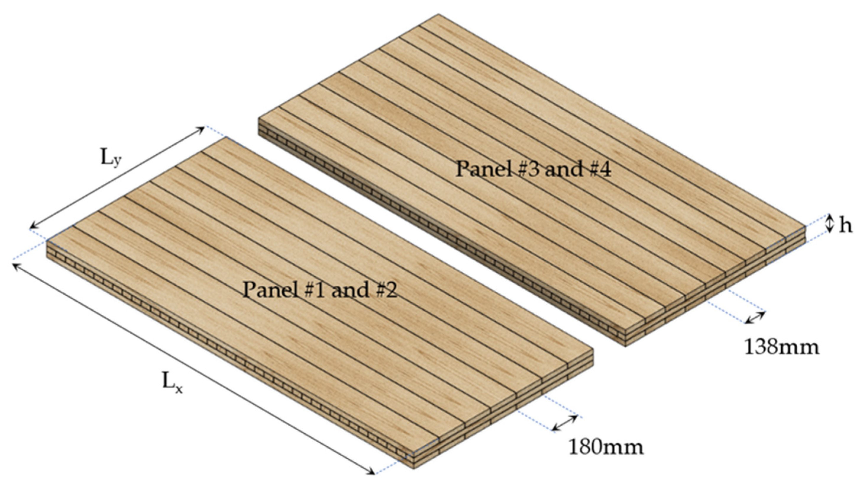
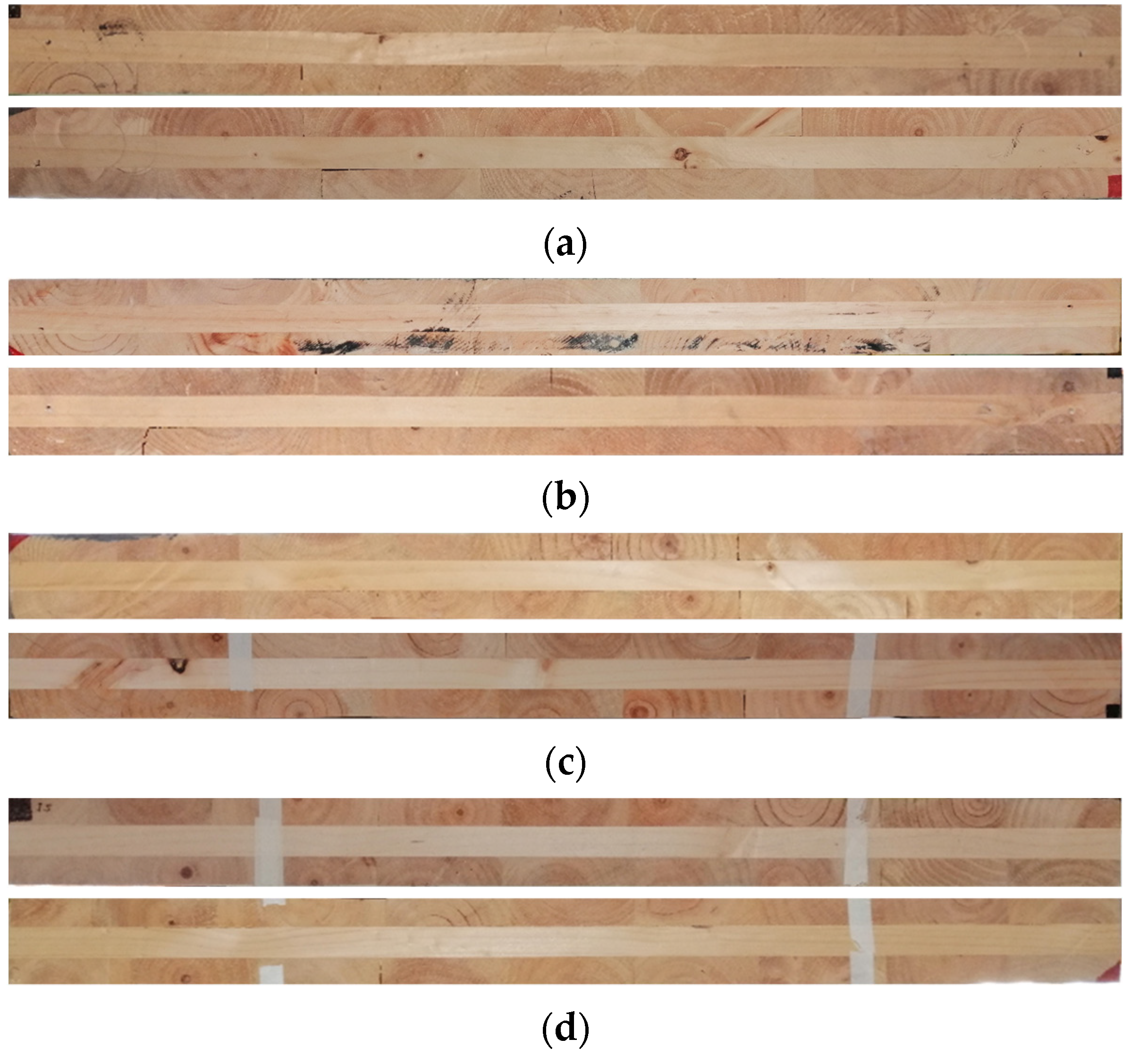
2.1.1. Description of the CLT Panels

Four 3-layer CLT panels were subjected to nondestructive transverse vibration testing. The panels were manufactured from low structural quality Pinus radiata boards, which had many defects such as knots, inclined fiber, and pith enclosed within the boards. These timber boards were mechanically classified in grade C16, which corresponds to the lowest structural quality allowed in the Chilean Standard for Wood Constructions [25]. According to the standard mentioned above, the average longitudinal modulus of elasticity of those C16-graded Radiata pine boards should vary between 6.9 GPa and 7.9 GPa. Therefore, the timber boards were bonded on their faces and edges with a polyurethane-type adhesive to achieve better structural performance. Figure 1 and

Table 1. Dimensions and physical properties of the CLT panels.

Panel #	Ly (mm)	Lx (mm)	h (mm)	Density (kg/m3)	Moisture Content (%)
1	1196.3	2596.0	96.3	451.9	11.2
2	1196.7	2580.3	96.1	457.1	12.8
3	1196.8	2598.0	96.9	441.7	12.2
4	1196.8	2596.3	96.8	442.3	11.1

summarize the panels’ geometric characteristics and some of their physical properties. In addition, Figure 2 and Figure 3 show the exterior faces and the cross-section (h × L_y) of the CLT panels, respectively.

From Table 1, Figure 2 and Figure 3, it can be seen that the three layers of the panels had similar thicknesses. However, panels #1 and #2 had wider outer boards (180 mm) than panels #3 and #4 (138 mm). In addition, the outer layers of panels #1 and #2 had a lower percentage of timber boards with enclosed pith (36%) than panels #3 and #4 (56%). All the above implies that panels #3 and #4 should have more juvenile wood (wood produced near the pith of the tree) and, therefore, lower global elastic properties than panels #1 and #2 [1].

2.1.2. Test Setup

The CLT panels were tested in a horizontal position (x–y plane), supported at four points. These supports were located at 22.4% of the length and width of the panels, measured from the edges. The reason for choosing these locations is that some relevant vertical vibration modes have zero modal amplitudes in the vicinity of these positions, achieving a boundary condition close to FFFF. In addition, the supports had high lateral stiffness (in the x- and y-directions) but low vertical stiffness (in the z-direction), thus minimizing the influence of the rigid body motion of the panels on their dynamic properties (Figure 4). This four-point supported test configuration was successfully used by Guan et al. [26] and Faircloth et al. [23] in the nondestructive evaluation of composite wood panels and CLT panels, respectively.

Once the boundary conditions of the test were known, the source of vibration excitation of the panels was defined. The panels were excited with a modal impact hammer (model 086D20, PCB Piezotronics, Depew, NY, USA), which had a soft tip to excite the frequency range of interest. The vertical impacts were applied at 45 points distributed on the top side of the panels, forming a five-by-nine rectangular grid (Figure 4). Each of these points was excited three times to average the transfer functions.

On the other hand, the structural vibrational response was measured by six integrated circuit piezoelectric (ICP) uniaxial accelerometers (model 603C01, IMI sensors, Depew, NY, USA). The accelerometers had a sensitivity of 100 mV/g, a broadband resolution of 0.00035 g, and were located on the panels’ bottom face. The data acquisition system consisted of a multi-channel dynamic signal acquisition module (model NI 9234) assembled into a Compact DAQ chassis (model cDAQ-9174, National Instruments, Austin, TX, USA) and linked via USB to a laptop. Finally, the vibrational response for each impact was sampled at a rate of 826 Hz, for a total of 8192 samples acquired, giving a frequency resolution of 0.101 Hz for an acquisition duration of 9.9 s. The typical test setup is shown in Figure 4.

2.2. Identification of CLT Panels’ Dynamic Properties

The test setup shown in the previous section allows identifying the most relevant resonant frequencies and the respective modal shapes of the CLT panels. According to Guan et al. [26], to estimate E_xx, E_yy, and G_xy in wood-based composite panels through a four-point supported transverse vibration test, it is necessary to obtain the resonant frequencies associated with three relevant vibration modes: ϕ₁, ϕ₂, and ϕ₃. A theoretical scheme of the vibration modes mentioned above is shown in Figure 5.

The frequencies and vibration modes were identified using the Polyreference Time Domain method (PTD), also called Polyreference Complex Exponential method (PRCE). This method was developed by Vold [27] and is one of the most widely used in practice because it even allows identifying closely spaced frequencies [28]. In addition, it works simultaneously with multiple references (e.g., multiple accelerometers), which generates a better estimation of the modal shapes.

In general terms, the PTD method extracts modal parameters of a system (e.g., poles and modal participation factors) from the modal decomposition in the time domain. The following steps are required to achieve its computational implementation:

• Select the impulse responses to be used for the extraction of modal parameters. The impulse responses relate an arbitrary impact point to an acceleration response reference point;
• Define a maximum limit for the order of the model or system. The model order corresponds to the number of poles to be identified in the system and is equal to twice the number of vibration modes to be considered;
• Construct the Hankel matrices. These matrices contain different arrays of impulse responses;
• Calculate the poles and modal participation factors for different model orders. These calculations must be done because the proper model order is not known a priori. One of the essential steps in this stage is to calculate a series of coefficients through a least-squares approximation. These coefficients are stored in a “companion matrix”, whose eigenvalues and eigenvectors allow us to calculate the poles and modal participation factors. Finally, from these poles and factors, the dynamic properties of the system can be estimated, i.e., its resonant frequencies, damping ratios, and modal shapes;
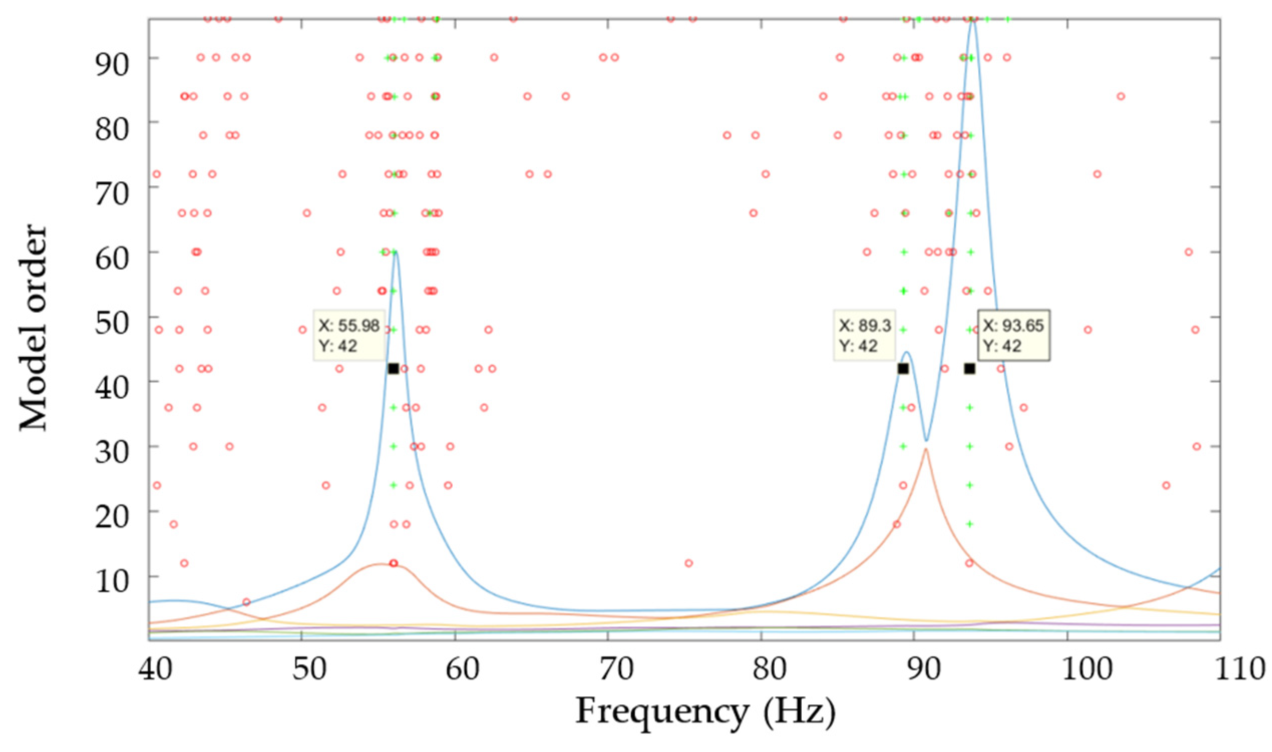
• Construct a stabilization diagram based on the estimates of poles and modal participation factors for the different model orders analyzed in the previous point. A typical stabilization diagram has a horizontal axis of frequencies and a vertical axis of model orders. Therefore, for a given model order value, the obtained poles are plotted along the frequency axis. If two poles at an order n and n + 1 of the model are within certain defined limits of frequency and damping, they are called “stable”;
• Select from the stabilization diagram the set of stable poles of interest. Finally, the frequencies and modal shapes of the system under study are obtained from these stable poles and their respective modal participation factors.

A typical example of a stabilization diagram generated by the PTD method is shown in Figure 6. More details of the PTD method can be found in [14,28]. The identification of all dynamic properties was performed in the ABRAVIBE toolbox [29].

2.3. Estimation of CLT Panels’ Elastic Properties

The finite element model updating technique, also known as a model calibration or parameter estimation [30], was used to estimate the variability of some elastic properties in the CLT panels. This technique allows the estimation of some unknown properties of a system, which are expressed as input parameters in a numerical model, from the measurement of other system properties by experimental tests. In the specific context of timber structures, the authors recently applied this methodology to study the local variability of the elastic properties of timber beams [31]. Based on the above, a two-phase methodology was implemented, as shown in Figure 7, and the two phases are described in detail below.

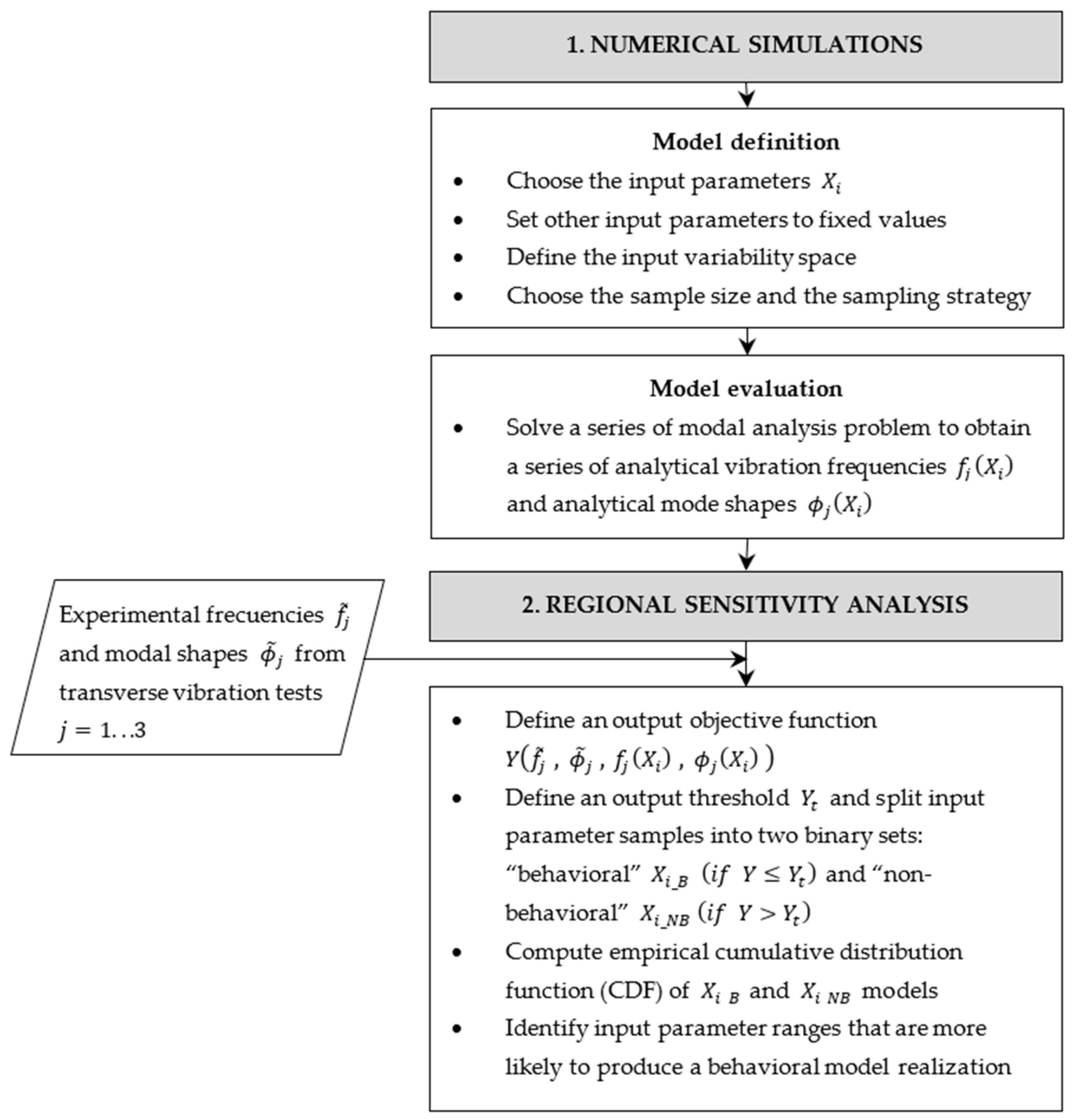
2.3.1. Numerical Simulations

The geometry, density, and support conditions of the CLT panels implemented in the experimental tests were replicated in numerical simulations using the finite element method. The numerical models were implemented in ETABS^® Ultimate software version 17 (New York, NY, USA) [32], using homogeneous shell elements, quadrilaterals of four nodes, and combining membrane and plate bending behaviors. For the homogenized CLT material, linear-elastic, orthotropic behavior was considered, incorporating shear deformations according to the Reissner–Mindlin theory.

When homogenized CLT is considered an orthotropic material, it is necessary to define nine elastic constants: three moduli of elasticity (E_xx, E_yy, E_zz), three shear moduli (G_xy, G_yz, G_xz), and three Poisson’s coefficients (v_xy, v_yz, v_xz). These elastic properties correspond to the input parameters of the model. If it is also of interest to know the spatial resolution of these properties within the panel, overparameterization along the structure should be avoided. The above is because overparameterization is the most common cause of ill-conditioning in model updating problems [30]. Therefore, it is advisable to use modeling strategies that minimize this type of problem, such as choosing physically relevant parameters and using substructures with constant parameters in adjacent element zones [30].

Based on the above, two simplifications were made to reduce the number of unknown model input parameters. The first simplification consisted of assuming that it is only necessary to accurately calculate three relevant homogenized elastic properties of CLT panels in most structural engineering applications: E_xx, E_yy, and G_xy. Therefore, the remaining elastic properties can be estimated either as constant values or as a function of the three relevant properties following the recommendations given in [17]. Applying these recommendations to three-layer CLT panels of equal thickness, we have $E_{zz}\approx E_{yy}, G_{xz}\approx 0.25G_{xy}, G_{yz}\approx 0.14G_{xy}, v_{xy}\approx 0.01, v_{xz}\approx 0.11, v_{yz}\approx 0.20$.

On the other hand, the second simplification assumed is that for practical structural engineering applications, it is sufficient to know the variability of the elastic properties within a CLT panel in rectangular macrozones, with dimensions between L_y/2 and L_x/4. This simplification was validated through interviews with professional experts in structural quality control of timber panels and preliminary numerical simulations to minimize the models’ possible overparameterization [33]. Thus, for the dimensions of the panels analyzed in this work, eight rectangular zones were considered, where the elastic properties were assumed to be constant. However, those eight zones were further divided into smaller zones to guarantee the proper discretization for applying the finite element method. In this way, it was possible to generate a finite element model with a dense mesh that allows us to obtain accurate results, but with eight zonal substructures of constant elastic properties that avoid problems of overparameterization. Finally, grouping the two simplifications mentioned above, it was concluded that 24 unknown input model parameters could be considered in the CLT panels studied (3 elastic properties defined in 8 different zones).

The variability space of the input parameters was estimated from the results of previous static tests on edge-glued CLT panels, carried out both in Chile [34] and other countries [8]. Thus, it was defined that E_xx could vary between 4.2 GPa and 10.1 GPa, E_yy between 0.4 GPa and 1.0 GPa, and G_xy between 0.3 GPa and 0.7 GPa.

The number of numerical model evaluations (sample size) should cover the whole range of variability of the input parameters adequately. In addition, the regional sensitivity analysis technique to be implemented requires the sample size to be at least 100 times the number of input parameters [35]. Therefore, a sample size of 2400 was chosen, with the Latin Hypercube sampling strategy [36]. Finally, the input parameters were assumed to be independent and uniformly distributed, following the recommendations given in [35]. Figure 8 shows in detail the numerical model used.

2.3.2. Regional Sensitivity Analysis

The numerical model mentioned above is complex because it has several input parameters with high variability. Therefore, in this type of model, the primary interest is not to find optimal values of the input parameters but rather to find acceptable ranges of variation for those parameters. One of the suitable methods to analyze this type of complex model is the Regional Sensitivity Analysis (RSA), also called Monte Carlo Filtering, and initially proposed by [37,38] in environmental quality studies. In general terms, RSA allows us to identify the regions where the input parameters of a model cause extreme values in a specific output variable.

In order to implement the RSA method, it is essential to define an output variable Y_(X), also called the objective function. This variable is a function of the input parameters stored in vector X. In this way, the Y_(X) values are calculated by varying all input parameters X simultaneously. Therefore, the sensitivity of each parameter considers not only its direct influence but also the joint influence due to interactions between the different parameters. This sampling strategy is called “All-[parameters]-At-a-Time” (AAT) and it is ideal for analyzing the results of complex models.

The principal utility of the variable Y_(X) in the RSA method is to divide the model parameters into two binary sets, “behavioral” (B) and “nonbehavioral” (NB). This division can be done by defining a set of maximum acceptable limits for Y_(X) called threshold values Y_t. In this work, Y_(X) is expressed as the difference between a set of dynamic properties measured in experimental tests and a set of the same properties calculated in numerical models. Therefore, the input parameters will belong to set B if they generate Y_(X) values less than the threshold values Y_t.

Previous research has focused on estimating the global average elastic properties of CLT panels, so it was only necessary to know the vibration frequencies of the panels. Thus, it was sufficient to define a simple objective function Y_(X) expressing the differences between the measured versus calculated frequencies in most of these investigations. However, when the goal of the study is to know the variability of the elastic properties in different zones, it is necessary to include in the objective function Y_(X) other dynamic properties such as modal shapes. The above is because the differences between the measured versus calculated modal shapes can better reflect local changes in the elastic properties of plate-like elements [39].

Combining these dynamic properties into a single objective function and a single threshold value is challenging because it is necessary to harmonize properties with very different dimensions and magnitudes. Sometimes it is possible to define a series of weighting factors that allow normalizing the different objective function components [31]; however, this process is tedious and indirectly increases the number of unknown parameters. Therefore, in the present work, it is proposed to apply three objective functions Y_(X) using both the frequencies and the modal shapes of the CLT panels. In addition, each objective function Y_(X) will have different threshold values Y_t, which will allow us to filter the models belonging to set B at different stages. The following steps are required to achieve the computational implementation of the proposal:

• Step 1: Apply a first objective function, $Y_{1\left(X\right)}$, shown in Equation (1), which is expressed as the average relative differences between the measured and calculated frequencies. The threshold value chosen for this function $Y_{1\left(X\right)}$ is $Y_{t1}=0.05$, which is compatible with the typical differences found by other researchers [23]. Therefore, B models will be filtered in this first stage as those generating vibration frequencies with less than 5% differences concerning the experimentally measured frequencies. This first filtering stage ensures that the B models have experimentally calibrated elastic property values at the global level of the panel;

$$Y_{1\left(X\right)}=\frac{1}{3}·{\displaystyle \sum }_{i=1}^3\left|\frac{{\tilde{\mathit{f}}}_i-{\mathit{f}}_{i\left(X\right)}}{{\tilde{\mathit{f}}}_i}\right|$$

(1)

where ${\tilde{\mathit{f}}}_i$ are the experimentally measured frequencies and ${\mathit{f}}_{i\left(X\right)}$ are the numerically calculated frequencies. All these frequencies are related to the three modal shapes shown in Figure 5.

• Step 2: Apply to the B models filtered in the previous stage a second objective function $Y_{2\left(X\right)}$, shown in Equation (2), expressed as the average Normalized Modal Difference (NMD) between the measured versus calculated modal shapes. Physically, NMD represents the fraction, on average, by which each degree of freedom (DOF) differs between two modal shapes. Besides, NMD can also be written in terms of another more popular modal shape correlation index called Modal Assurance Criterion (MAC). Thus, for example, if each DOF had an average error of 10%, the MAC and NMD values would be 0.99 and 0.1, respectively. Detailed analytical expressions of MAC and NMD can be found in [14]. According to [2], a MAC value greater than 0.95, or its corresponding NMD value less than 0.2, indicates a good correlation between two modal shapes associated with a CLT panel. Therefore, the threshold value chosen for this function $Y_{2\left(X\right)}$ is $Y_{t2}=0.20$. In summary, this second filtering stage ensures that the B models have modal shapes similar to those measured experimentally at the global level;

$$Y_{2\left(X\right)}=\frac{1}{3}{\displaystyle \sum }_{i=1}^{3}NMD\left({\tilde{\mathit{\varphi }}}_i,{\mathit{\varphi }}_{i\left(X\right)}\right)=\frac{1}{3}{\displaystyle \sum }_{i=1}^3\sqrt{\left[1-MAC\left({\tilde{\mathit{\varphi }}}_i,{\mathit{\varphi }}_{i\left(X\right)}\right)\right]/MAC\left({\tilde{\mathit{\varphi }}}_i,{\mathit{\varphi }}_{i\left(X\right)}\right)}$$

(2)

where ${\tilde{\mathit{\varphi }}}_i$ are the experimentally measured modal shape vectors, and ${\mathit{\varphi }}_{i\left(X\right)}$ are the numerically calculated modal shape vectors (Figure 5), MAC is the Modal Assurance Criterion, and NMD is the Normalized Modal Difference.

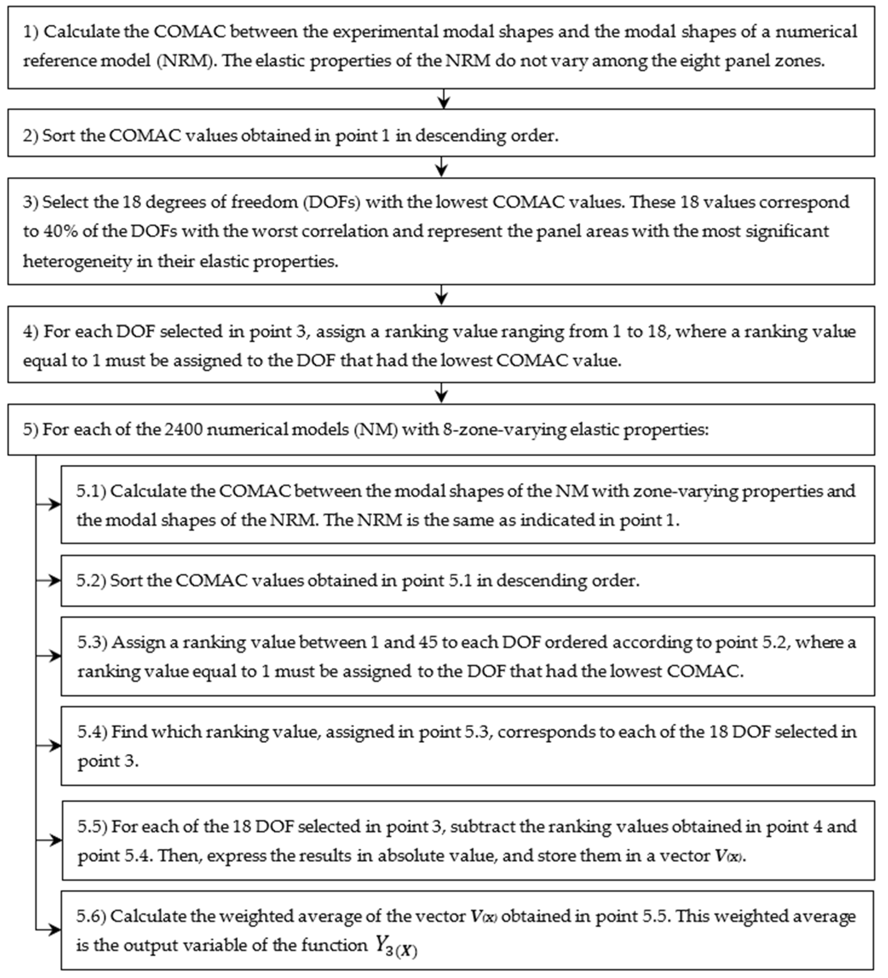
• Step 3: Apply a third objective function $Y_{3\left(X\right)}$ to the B models filtered in step 2. This function $Y_{3\left(X\right)}$, unlike the functions $Y_{1\left(X\right)}$ and $Y_{2\left(X\right)}$, should have a strong emphasis on the local variability of the elastic properties. Therefore, it is convenient that $Y_{3\left(X\right)}$ is expressed in terms of the modal shapes’ DOFs that deviate most from specific ideal reference values. A suitable indicator for this type of spatial error distribution is the Coordinate Modal Assurance Criterion (COMAC). COMAC measures the correlation at each DOF averaged over a set of paired experimental–numerical modal shapes. In each DOF, the COMAC values can vary between 0 and 1, where 1 implies perfect correlation. Detailed analytical expressions of COMAC can be found in [14]. The calculation procedure of the function $Y_{3\left(X\right)}$ is shown in Figure 9.

As indicated in point 5.6 of the procedure shown in Figure 9, the output variable of the function $Y_{3\left(X\right)}$ corresponds to the weighted average of the vector V_(X), as shown in Equation (3):

$$Y_{3\left(X\right)}={\displaystyle \sum }_{i=1}^{18}{W}_i·V_{i\left(X\right)}$$

(3)

where V_(X) is a vector that contains the COMAC ranking differences for the 18 selected DOFs mentioned in Figure 9. Besides, W_i are the weighting factors defined according to Equation (4):

$$W_i=i/{\displaystyle \sum }_{j=1}^{18}j$$

(4)

From Equation (4), the weighting factors vary linearly from 1/171 for the DOF that had the highest COMAC value of the 18 DOFs selected in point 3 (Figure 9) to 18/171 for the DOF that had the lowest COMAC value. Therefore, the output variable $Y_{3\left(X\right)}$ represents, on average, how many positions a given numerical model errs in ordering the most relevant modal DOFs concerning the experimental modal shapes. The threshold value chosen for this function $Y_{3\left(X\right)}$ is $Y_{t3}=11$, which corresponds to approximately 33% of the maximum possible value of $Y_{3\left(X\right)}$. Then, this last filtering step ensures that the B models have a variability of their elastic properties among the different panel zones like the variability obtained experimentally.

It is worth mentioning that the three objective functions can be applied in any order. The above mention is because the B models must simultaneously meet the three constraints imposed by the threshold values. In addition, it is essential to emphasize that the ranges of values of the elastic properties used in the numerical models must be representative of the type of panel analyzed because this initial selection may influence the filtering process of the B models.

Once the models have been separated into sets B and NB, their input parameters’ empirical cumulative distribution functions (CDFs) are calculated and plotted. Then, the Kolmogorov–Smirnov (K–S) test is used to evaluate whether there are statistically significant differences between the CDFs of sets B and NB. If the K-S test indicates significant differences between the CDFs, a statistical distribution that fits the input parameters of the B models is identified. The aforementioned statistical adjustment allows an in-depth analysis of the ranges of variation of the elastic properties and their subsequent comparison with normative limits. The SAFE toolbox [40] was used to perform the computational implementation of the RSA model.

3. Results and Discussion

3.1. Experimental Dynamic Properties of the CLT Panels

The experimental frequencies obtained for the four panels are shown in

Table 2. Experimental frequencies of CLT panels.

Panel #	${\tilde{\mathit{f}}}_1\left(\mathbf{Hz}\right)$	${\tilde{\mathit{f}}}_2\left(\mathbf{Hz}\right)$	${\tilde{\mathit{f}}}_3\left(\mathbf{Hz}\right)$
1	56.06 (0.11%)	89.30 (0.04%)	93.69 (0.05%)
2	56.12 (0.09%)	91.83 (0.10%)	95.75 (0.06%)
3	51.74 (0.11%)	93.76 (0.11%)	96.40 (0.06%)
4	49.61 (0.13%)	92.52 (0.08%)	96.98 (0.05%)

The coefficients of variation of the frequencies are shown in parenthesis.

. In addition, Figure 10, Figure 11 and Figure 12 show the experimental modal shapes of the panels.

From Table 2, it can be seen that panels #1 and #2 had on average 10% higher ${\tilde{\mathit{f}}}_1$ frequencies than panels #3 and #4. These results suggest that panels #1 and #2 should have higher E_xx moduli of elasticity in global terms than panels #3 and #4. The above mention is confirmed by the fact that panels #1 and #2 were made of exterior timber boards of higher structural quality, as shown in Section 2.1.1. In addition, panels #1 and #2 had fewer timber boards per unit width in their outer layers than panels #3 and #4, so it was expected that the homogenized E_xx properties of panels #1 and #2 would be less affected by the local variability of their timber boards. However, for the frequencies ${\tilde{\mathit{f}}}_2$ and ${\tilde{\mathit{f}}}_3$, a different trend occurred because, according to Table 2, panels #1 and #2 had on average 3% and 2% lower values than panels #3 and #4. Therefore, the overall values of E_yy and G_xy are expected to be more uniform among all the evaluated panels. Finally, it should be noted that the coefficients of variation obtained for the different frequencies were very low, which gives greater statistical validity to the results obtained.

On the other hand, Figure 10, Figure 11 and Figure 12 show that the experimentally measured modal shapes matched the expected theoretical modal shapes (shown in Figure 5). Furthermore, if these figures are only observed at the global level, it could be wrongly deduced that there are no relevant differences between the modal shapes of different panels. However, when analyzing each DOF of the modal shapes at the local level, relevant differences were found between the different panels. For example, when comparing ${\tilde{\mathit{\varphi }}}_1$ from panels #1 and #4, 60% of the DOFs differed between 20% and 100% in their amplitudes. These results suggest that the local variability of the elastic properties may be distributed differently among the different panels.

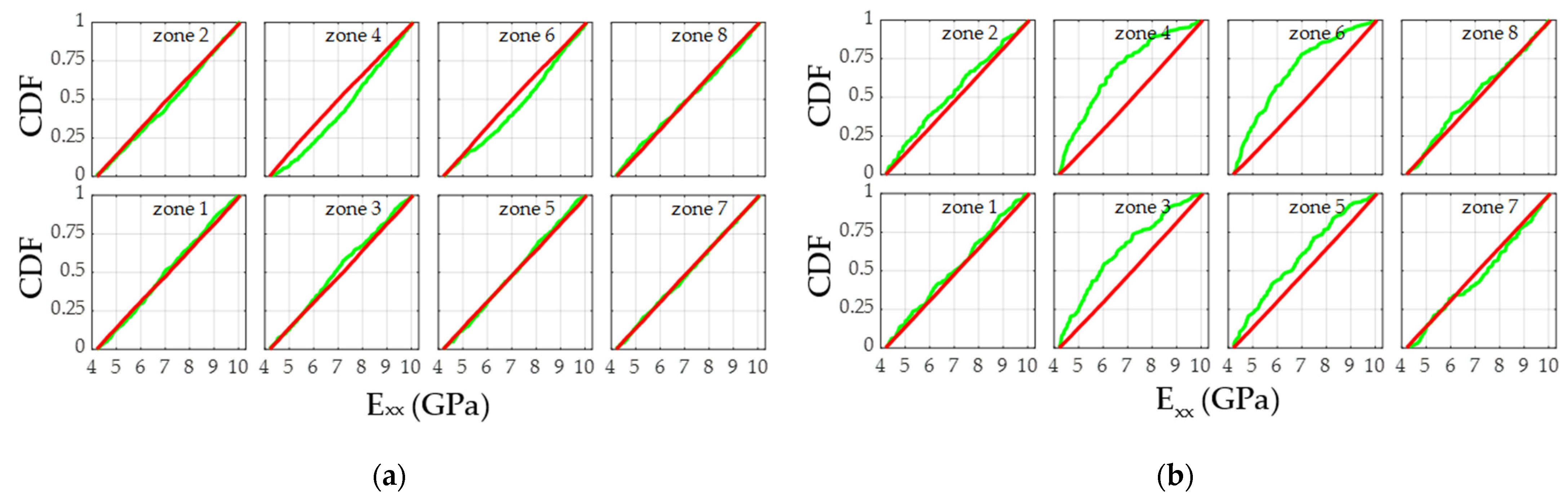
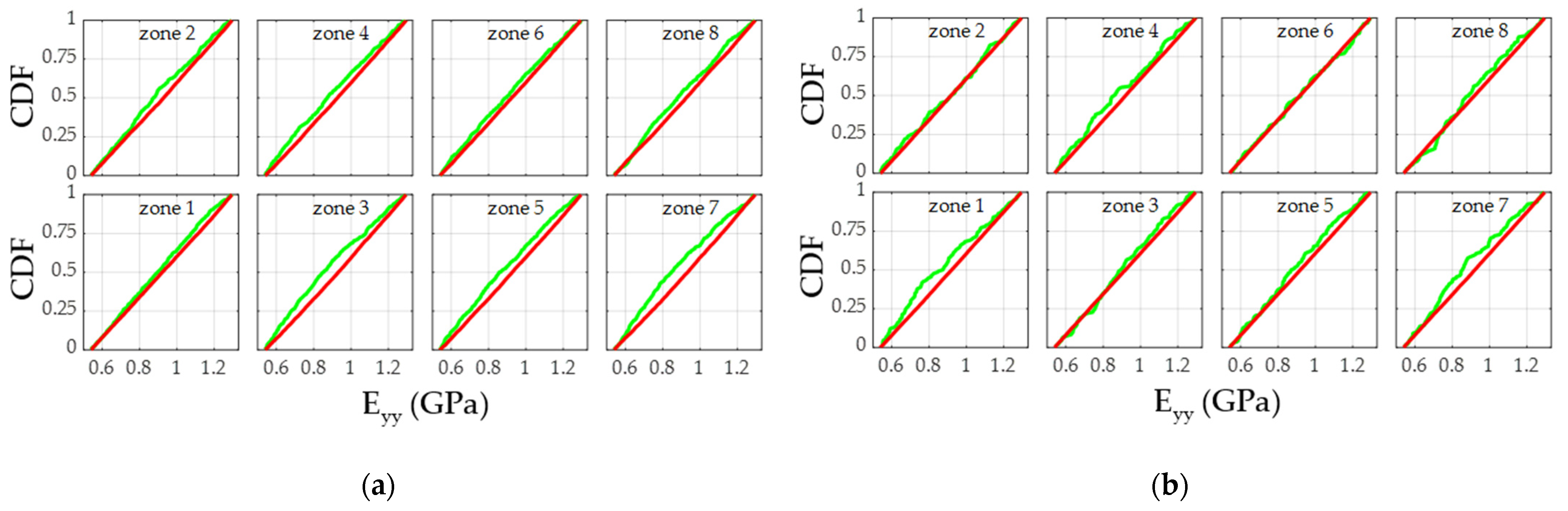
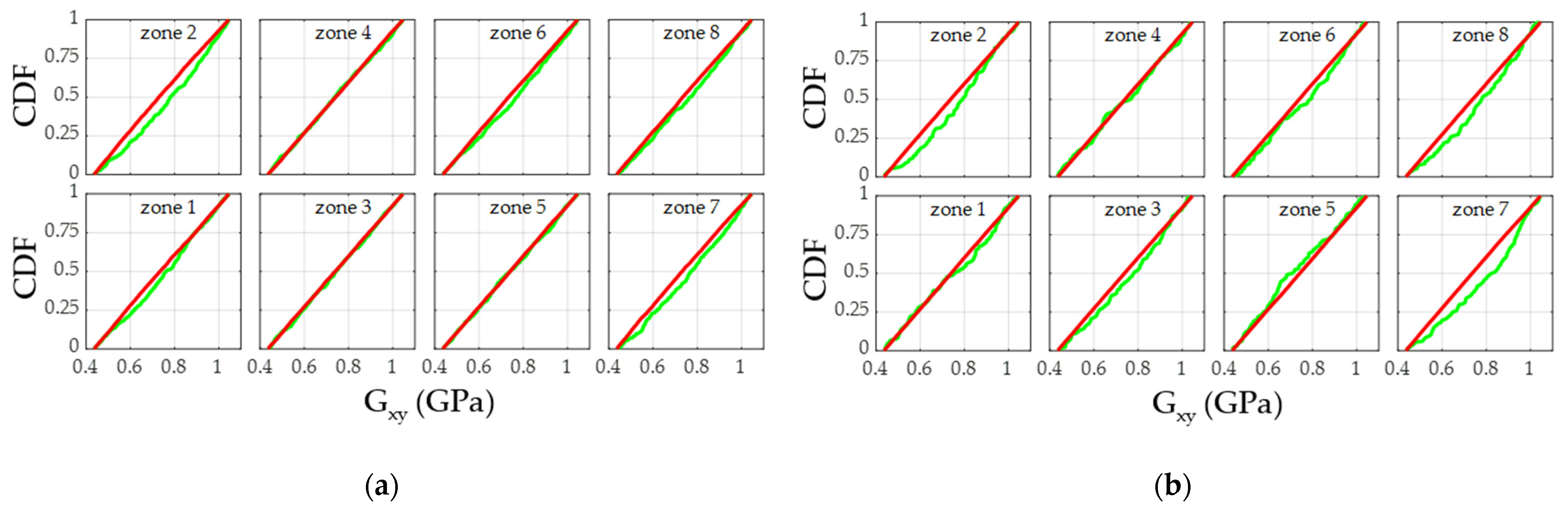
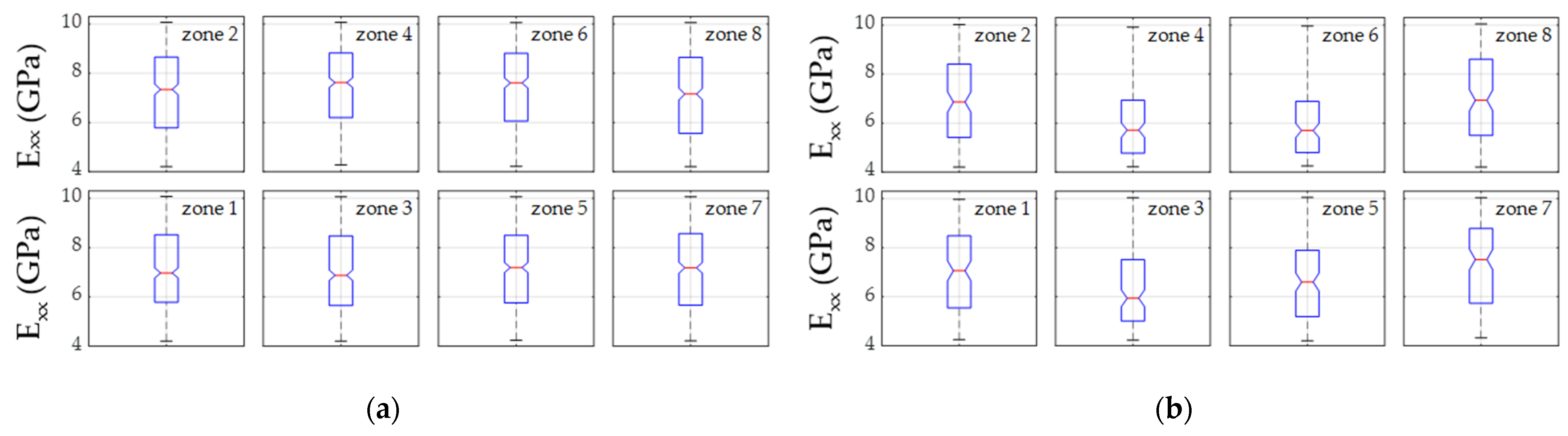
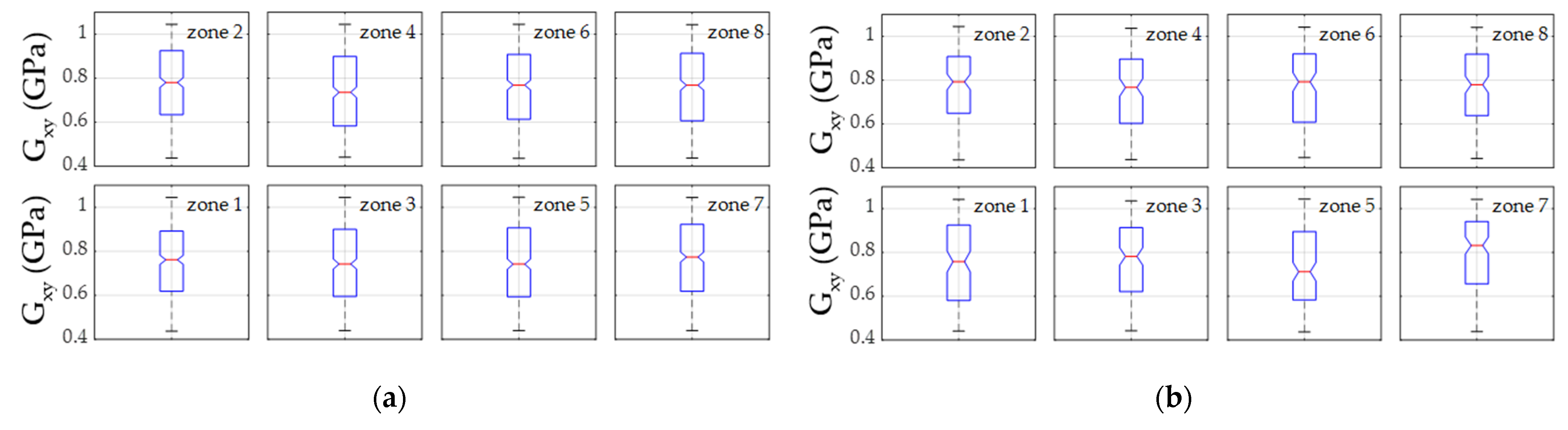
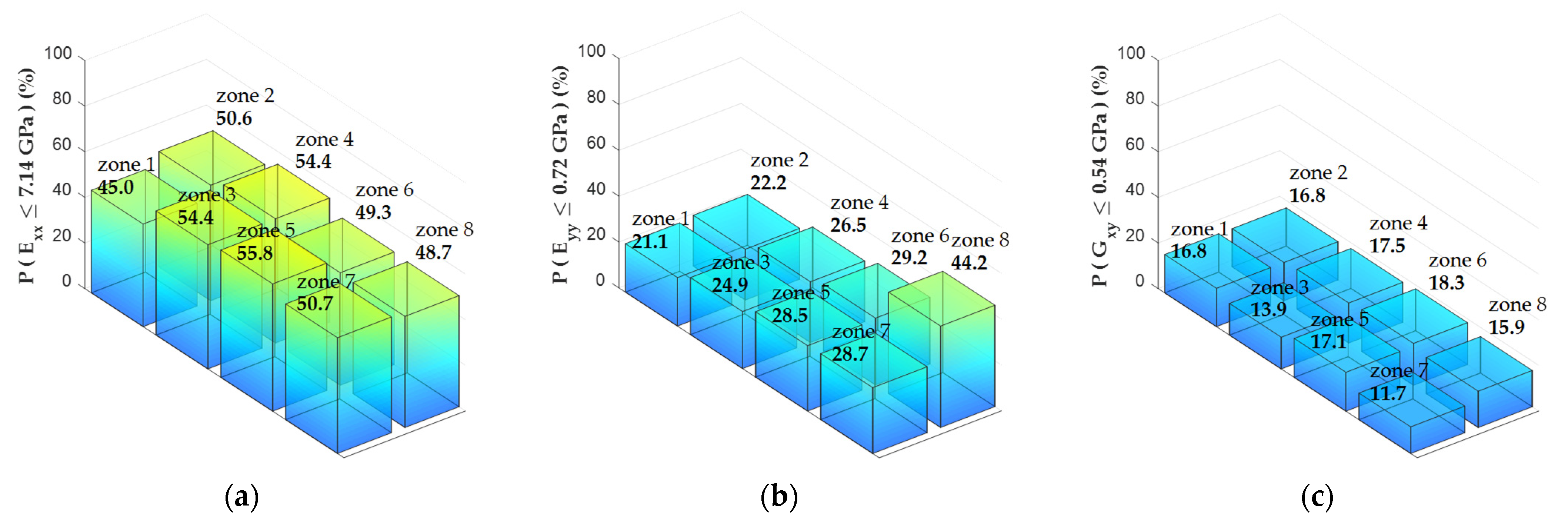
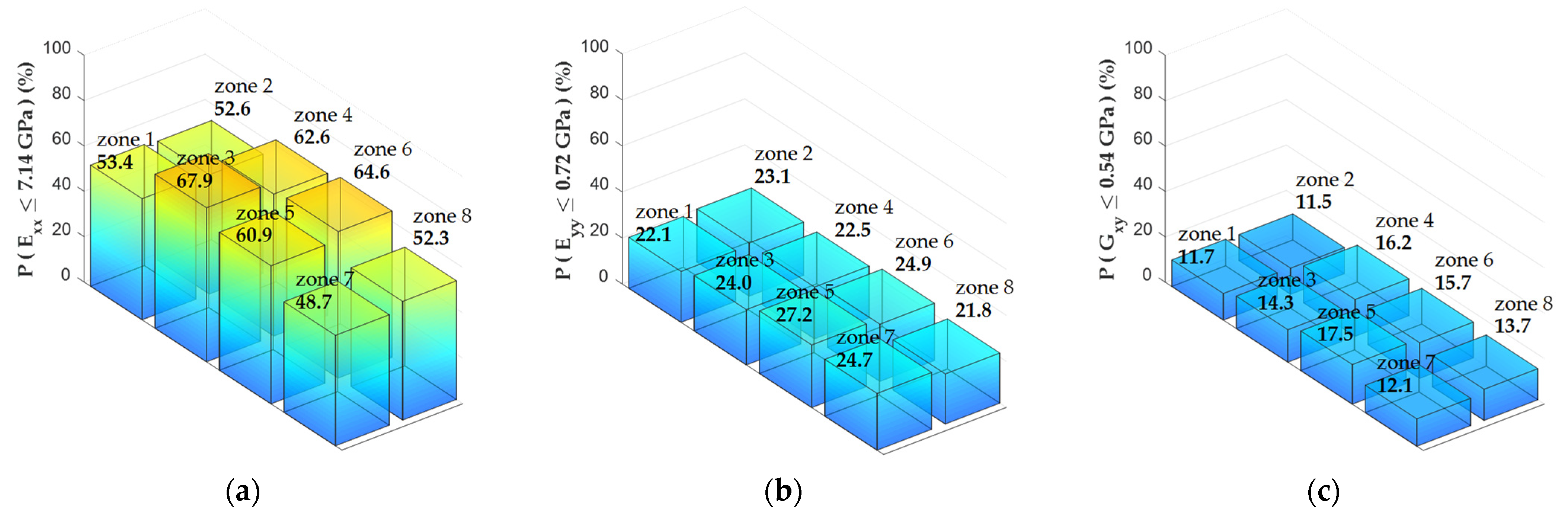
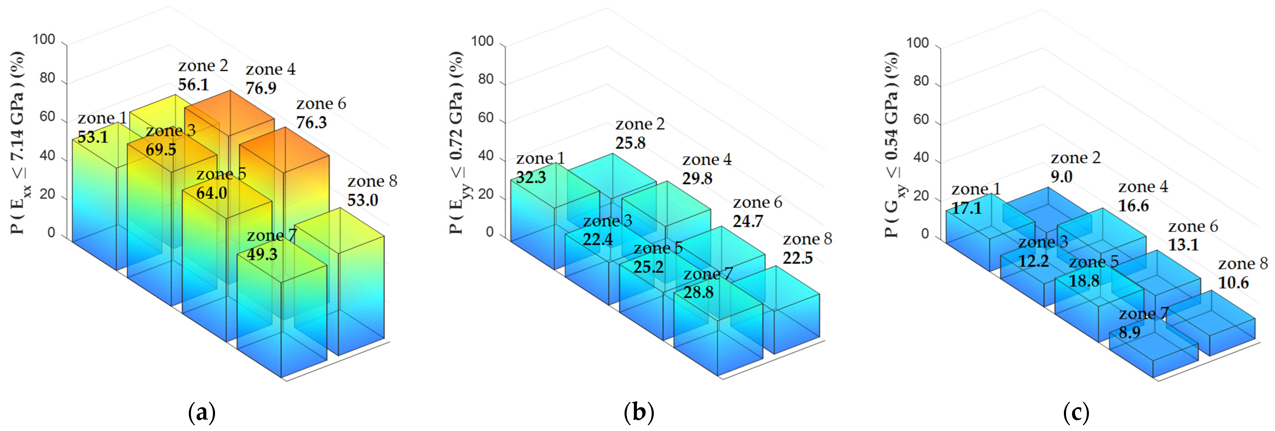
3.2. Local Variability of the Elastic Properties

Once the most relevant dynamic properties of the CLT panels were calculated, the numerical simulations and the subsequent sensitivity analysis were performed, as indicated in Section 2.3.

Table 3. Main results of numerical simulations.

Panel #	Number of Simulations	Number of B Models	Number of NB Models	Mean Value of the Objective Functions in B Models
				${\mathit{Y}}_{1\left(\mathit{X}\right)}$	${\mathit{Y}}_{2\left(\mathit{X}\right)}$	${\mathit{Y}}_{3\left(\mathit{X}\right)}$
1	2400	440	1960	0.032	0.165	9.27
2	2400	203	2197	0.033	0.163	9.73
3	2400	418	1982	0.036	0.183	4.29
4	2400	132	2268	0.041	0.182	5.81

shows the number of models that fell into the B (behavioral) and NB (nonbehavioral) categories, together with the average values obtained in the three objective functions for the B models.

The results shown in Table 3 indicate that only a small percentage of the total models were in category B, varying between 6% and 18%. This situation is quite common in RSA regional sensitivity analyses because this method aims to find the ranges of variation of the model parameters that significantly influence the output variables or objective functions. Thus, it is observed that only a select group of the simulated models achieved a reasonable degree of fit concerning the dynamic properties obtained experimentally.

On the other hand, the mean values obtained in the objective functions of the B models showed interesting trends. Panels #3 and #4 had larger average values of $Y_{1\left(X\right)}$ and $Y_{2\left(X\right)}$, which implies that their B models had a more challenging overall fit to the experimental values of frequencies and modal shapes. Besides, these same panels also had smaller $Y_{3\left(X\right)}$ values, which means they had less difficulty detecting zones with high local variability in the modal shapes. All these results suggest that panels #3 and #4 may have elastic properties of lower magnitude and higher local variability than panels #1 and #2.

To better visualize the above-mentioned, Figure 13, Figure 14, Figure 15, Figure 16, Figure 17 and Figure 18 show different ways of representing the ranges of variation of the elastic properties obtained in the B models. Only the results of panels #1 and #4 are shown because they correspond to extreme cases that allow analyzing the methodologies’ validity.

The CDF plots in Figure 13, Figure 14 and Figure 15 allowed analyzing the zonal influence of E_xx, E_yy, and G_xy on the output variable Y (represented by the simultaneous application of the objective functions Y_1(X), Y_2(X), and Y_3(X)). A simplified way to visualize whether an input parameter belongs to the critical sensitivity class is that the CDF coming from its B models (green lines) is separated from the CDF coming from its NB models (red lines).

According to the RSA method, the influence of an input parameter (e.g., E_xx, E_yy, and G_xy zones) on the output variable Y can also be estimated by applying the Kolmogorov–Smirnov (K–S) test to the CDFs coming from its B and NB models. Consequently, the lower the p-value obtained of the K–S test, the more influential the input parameter is on the output variable. Therefore, some authors [41] suggest that the input parameters can be grouped into three sensitivity classes: critical “C” (p-value < 0.01), important “I” (0.01 < p-value < 0.1), and negligible “N” (p-value > 0.1).

Table 4. Sensitivity classes for CLT panels #1 and #4.

Panel #	Elastic Property	Zone 1	Zone 2	Zone 3	Zone 4	Zone 5	Zone 6	Zone 7	Zone 8
1	Exx	N (0.44)	N (0.16)	I (0.02)	C (<0.001)	N (0.49)	C (<0.001)	N (0.93)	N (0.46)
1	Eyy	N (0.12)	C (0.004)	C (<0.001)	I (0.01)	C (0.002)	N (0.19)	C (<0.001)	I (0.04)
1	Gxy	I (0.03)	C (<0.001)	N (0.74)	N (0.90)	N (0.71)	I (0.04)	C (0.003)	I (0.09)
4	Exx	N (0.59)	N (0.27)	C (<0.001)	C (<0.001)	C (0.002)	C (<0.001)	N (0.28)	N (0.32)
4	Eyy	I (0.03)	N (0.89)	N (0.68)	N (0.21)	N (0.45)	N (0.86)	I (0.03)	N (0.47)
4	Gxy	N (0.28)	I (0.03)	N (0.28)	N (0.81)	N (0.28)	N (0.19)	C (0.001)	I (0.03)

The p-values are shown in parenthesis.

shows the sensitivity classes obtained for panels #1 and #4.

The results shown in Table 4 allow detecting which zones in a panel are more relevant to analyze more in-depth, from the point of view of the variability of their elastic properties, concerning the range of variation initially chosen. For example, suppose that a negligible sensitivity class was assigned to some zone. In that case, it means the B models in that zone have an almost uniform distribution of elastic property values over the whole range of variation initially defined. On the other hand, if a critical or an important sensitivity class was assigned in another zone, it means that the B models in that zone generated a distribution of values different from the original uniform one. However, to know whether the distribution of values was more concentrated towards the maximum or minimum extremes of the original range of variation, it is advisable to analyze the boxplots of the values obtained in the B models. Figure 16, Figure 17 and Figure 18 show the boxplots of the elastic properties for panels #1 and #4.

The boxplots in Figure 16, Figure 17 and Figure 18 indicate how the ranges of values of the most influential input parameters from the B models were distributed. In addition, the notches indicated in these boxplots allow a rough estimate of the median confidence interval of each input parameter. Therefore, comparing the notches in the different panel zones allows us to roughly estimate whether there are statistically significant differences of an elastic property within a panel. For example, when comparing the boxplots obtained for E_xx in the different zones of panel #4 (Figure 16b), it can be observed that the notches do not coincide. Therefore, this situation suggests a high local variability of E_xx in that panel.

In this way, combining CDF curve plots and boxplots makes it possible to know how influential an elastic property is in a panel zone, and towards which range of values its influence is concentrated. For example, Figure 13a shows that for panel #1, the variable E_xx in zone 4 is one of the most influential, as the CFDs coming from its models B and NB are separated. If we also check the boxplot in Figure 16a in the same zone 4, we can see that the influence of E_xx is concentrated towards a range of higher E_xx values. Another relevant example can be seen in Figure 13b. It is observed that for panel #4, the E_xx property is very influential in zones 4 and 6, given the evident separation between the CDFs of sets B and NB. In this case, when observing Figure 16b, the influence of E_xx is concentrated towards a lower range of values, which could indicate the presence of relevant defects in that zone of the panel. This type of analysis allows the generation of new structural quality control criteria for CLT panels, as discussed in the following subsection.

3.3. Applications for Structural Quality Control of CLT Panels

Some probabilistic criteria of structural acceptance or rejection can be studied in greater depth with the CDF curves of the elastic properties coming from the B models. The first step is to identify a probability distribution that fits well with the CDFs of the B models. The above-mentioned was done through the Minitab software quality tools [42], where the Johnson transformation [43] was identified as the best fit to the B models. This transformation is widely used in statistical process control as it allows any quality indicator to be fitted to a normal distribution. Figure 19 shows some examples of the fits achieved in the CDFs of some elastic properties with important or critical sensitivity.

The second step is to define a set of target acceptable values for specific elastic properties of the panels. One of the ways to obtain these target values is through theoretical equations compatible with the type of panel studied. Because the present investigation used edge-bonded CLT panels, the k-method was chosen to estimate the acceptable E_xx, E_yy, and G_xy values. The k-method is based on the theory of composite materials and estimates the elastic properties of the panels globally from the nominal elastic properties of the timber boards that compose the panel. The Chilean Wood Construction Standard [25] was used to obtain the average nominal values of Radiata pine boards. Therefore, applying the k-method for three-layer CLT panels, average target values of 7.14 GPa, 0.72 GPa, and 0.54 GPa were obtained for E_xx, E_yy, and G_xy, respectively.

Finally, knowing the information indicated in the previous paragraphs, it is possible to estimate the probability that a CLT panel has local elastic properties lower than average target values in a specific zone. These probabilities allow more reliable decisions to be made regarding the structural quality control of CLT panels. Figure 20, Figure 21, Figure 22 and Figure 23 show the probabilities obtained for all the CLT panels analyzed.

Several trends can be highlighted from the results obtained in Figure 20, Figure 21, Figure 22 and Figure 23. The first trend was that the elastic properties with the highest probabilities of not exceeding the average target values were the E_xx in the different panels. The non-exceedance probabilities ranged from 41.3% to 76.9%, 21.2% to 44.2%, and 8.9% to 18.8% for E_xx, E_yy, and G_xy, respectively. Therefore, in the CLT panels analyzed, the most relevant elastic properties from the point of view of structural quality control are E_xx in the different zones.

Another trend detected was that the E_xx non-exceedance probabilities were higher in panels #3 and #4 compared to panels #1 and #2. While in panels #1 and #2, the E_xx probabilities remained below 53.3% and 55.8%, respectively, in panels #3 and #4, they reached higher values, on the order of 67.9% and 76.9%, respectively. As mentioned in Section 2.1.1, these results were expected because panels #3 and #4 had a higher percentage of timber boards with enclosed pith, which generally implies lower elastic properties.

The last trend detected was the ability of the proposed method to indicate the zones of the CLT panels that had the most difficulty in satisfying E_xx structural quality standards. The ability mentioned above was most evident in the four central zones of the panels (zones 3 to 6). These central zones are critical in most structural wall or slab applications with CLT panels because they are generally not as restricted in movement as the outer panel zones. Accordingly, this implies that the central zones of CLT panels could control the structural design for serviceability limit states (e.g., excessive displacements and vibrations).

A clear example of that mentioned in the previous paragraph was the results obtained in panel #4. The E_xx non-exceedance probabilities were 69.5%, 76.9%, 64.0% and 76.3% for zones 3 to 6, respectively (Figure 23a). Besides, a good correlation can be seen by contrasting the probabilities with the pictures of those zones’ top and bottom faces in panel #4 (Figure 24). In fact, the highest probabilities of not exceeding were obtained in zones 4 and 6, which is logical because the presence of pith in timber boards were strong, both in the top and bottom faces. On the other hand, in zone 3, the probability of not exceeding was a little lower than in zones 4 and 6 because there is only the presence of pith on one of the panel’s faces. Finally, in zone 5, the probability trend continued downward because of the four zones analyzed; it was the one with the lowest presence of pith.

The negative effect of manufacturing CLT panels with timber boards containing pith can also be analyzed with the mean values obtained in E_xx for B models in the different zones of panel #4. After applying the Johnson transformation to the E_xx CDF curves (B models), the mean value in each zone could be calculated. For zones 3 to 6, mean E_xx values of 5.96 GPa, 5.66 GPa, 6.26 GPa, and 5.70 GPa were obtained. Therefore, in the worst case (zone 4), E_xx mean value is 21% lower than the average target value of 7.14 GPa. This percentage of variation is quite logical because the average target value considers that the timber boards that make up the CLT panel do not have pith presence. Therefore, because there were timber boards with pith in the central zones of panel #4, even in the two outer layers simultaneously, this local reduction was to be expected. Additionally, the orders of magnitude of the reductions in E_xx were reasonable because recent research [44] has shown that in certain softwoods, the global static elasticity modulus can be up to 25% lower in “core-wood” boards (with pith presence) than in “outer-wood” boards (without pith presence).

In summary, considering all the above results, it is possible to propose an acceptance criterion for CLT panels based on the estimation of their elastic properties by zones. The philosophy behind this criterion is that it is not enough for a panel to have adequate global elastic properties; it is also desirable that it does not show significant decreases at the local level. The target values for the elastic properties of CLT panels generally correspond to acceptable average values; therefore, if in a panel the probabilities of not exceeding those target values are less than 50%, that panel is expected to have adequate stiffness under service conditions. On the other hand, if the probabilities of not exceeding are greater than 50%, the panel could present future serviceability problems. Based on the above, it is necessary to define an upper limit for the non-exceedance probability, which allows the rejection of panels with decreased elastic properties in their central zones. For example, a reasonable limit could be the non-exceedance probability of 65% in the central zones. The panel zones that exceeded this limit had mean values of elastic properties between 12% and 21% lower than the average target values. From this perspective, panels #1 and #2 meet the structural quality control criterion, while panels #3 and #4 do not. Thus, a proposal of this type could improve both the manufacturing and quality control processes of CLT panels with low structural quality wood boards, generating an adequate balance between sustainability and structural performance under service loads.

4. Conclusions

This paper has highlighted the importance of the nondestructive assessment of low-grade CLT panels’ elastic properties. Furthermore, the experimental and numerical campaign revealed ranges of local elastic properties for this kind of CLT panels by applying transverse vibration tests and finite element models. Thus, the type of CLT panels studied, combined with experimental modal analysis, numerical simulations, and regional sensitivity analysis, makes this research especially novel and contributes to extending the current knowledge in the timber industry.

The results obtained suggest that the elastic properties’ local variability could be a better stiffness-based quality indicator than the traditional global elastic properties, especially for low-grade CLT panels. Accordingly, a good indicator was the probability of not exceeding an elastic property average target value in the CLT panels’ central zones. Generally, when this probability of non-exceedance was greater than 65%, it coincided with that panel zone having relevant defects (e.g., presence of pith) in both the top and bottom layered timber boards simultaneously. Therefore, the above probability limit was a good indicator for structural quality control of CLT panels to prevent future serviceability problems in buildings constructed with these panels.

Finally, the results of this study support the idea that low-grade CLT panels could be used as structural elements promoting more sustainable constructions. However, because it is common for these panels to present a significant number of defects, it is essential to select only those with low local variability in their bending stiffness to avoid future complaints by users. To overcome these challenges, the nondestructive evaluation method presented in this study proved to be very useful. Therefore, future work will investigate low-grade CLT panels of different structural configurations and technologies that allow faster nondestructive assessments in both laboratory and in situ contexts.

References

1. Ross, R.J. Wood Handbook: Wood as an Engineering Material; General Technical Report FPL-GTR-190; U.S. Department of Agriculture, Forest Service, Forest Products Laboratory: Madison, WI, USA, 2010.
2. Gsell, D.; Feltrin, G.; Schubert, S.; Steiger, R.; Motavalli, M. Cross-Laminated Timber Plates: Evaluation and Verification of Homogenized Elastic Properties. J. Struct. Eng. 2007, 133, 132–138. [Google Scholar] [CrossRef]
3. Steiger, R.; Gülzow, A.; Czaderski, C.; Howald, M.T.; Niemz, P. Comparison of Bending Stiffness of Cross-Laminated Solid Timber Derived by Modal Analysis of Full Panels and by Bending Tests of Strip-Shaped Specimens. Eur. J. Wood Prod. 2012, 70, 141–153. [Google Scholar] [CrossRef] [Green Version]
4. Lukacs, I.; Björnfot, A.; Tomasi, R. Strength and Stiffness of Cross-Laminated Timber (CLT) Shear Walls: State-of-the-Art of Analytical Approaches. Eng. Struct. 2019, 178, 136–147. [Google Scholar] [CrossRef]
5. Bodig, J.; Jayne, B. Mechanics of Wood and Wood Composites, 1st ed.; Krieger Publishing Company: Melbourne, FL, USA, 1982. [Google Scholar]
6. EU. Eurocode 5 Design of Timber Structures. Part 1-1: General Common Rules and Rules for Buildings; EN 1995-1-1; CEN: Brussels, Belgium, 2006. [Google Scholar]
7. Kreuzinger, H. Plate and Shell Structures. A Model for Common Calculation Tools. Bauen Mit Holz 1999, 1, 34–39. [Google Scholar]
8. Zhou, J.; Chui, Y.H.; Gong, M.; Hu, L. Elastic Properties of Full-Size Mass Timber Panels: Characterization Using Modal Testing and Comparison with Model Predictions. Compos. Part B-Eng. 2017, 112, 203–212. [Google Scholar] [CrossRef]
9. Bos, F.; Casagrande, S.B. On-Line Non-Destructive Evaluation and Control of Wood-Based Panels by Vibration Analysis. J. Sound Vib. 2003, 268, 403–412. [Google Scholar] [CrossRef]
10. Zhang, L.; Tiemann, A.; Zhang, T.; Gauthier, T.; Hsu, K.; Mahamid, M.; Moniruzzaman, P.K.; Ozevin, D. Nondestructive Assessment of Cross-Laminated Timber Using Non-Contact Transverse Vibration and Ultrasonic Testing. Eur. J. Wood Prod. 2021, 79, 335–347. [Google Scholar] [CrossRef]
11. Ross, R.J. Nondestructive Evaluation of Wood, 2nd ed.; General Technical Report FPL-GTR-238; U.S. Department of Agriculture, Forest Service, Forest Products Laboratory: Madison, WI, USA, 2015.
12. Ross, R.J.; Geske, E.; Larson, G.; Murphy, J. Transverse Vibration Nondestructive Testing Using a Personal Computer; Research Paper FPL-RP-502; U.S. Department of Agriculture, Forest Service. Forest Products Laboratory: Madison, WI, USA, 1991.
13. Murphy, J. Transverse Vibration of a Simply Supported Beam with Symmetric Overhang of Arbitrary Length. J. Test. Eval. 1997, 25, 522–524. [Google Scholar]
14. Maia, N.M.M.; Silva, J.M.M. Theoretical and Experimental Modal Analysis, 1st ed.; Research Studies Press Ltd.: Baldock, Hertfordshire, UK, 1997. [Google Scholar]
15. Rainieri, C.; Fabbrocino, G. Operational Modal Analysis of Civil Engineering Structures, 1st ed.; Springer: New York, NY, USA, 2014. [Google Scholar]
16. Brincker, R.; Ventura, C. Introduction to Operational Modal Analysis, 1st ed.; John Wiley & Sons: Hoboken, NJ, USA, 2015. [Google Scholar]
17. Gülzow, A.; Gsell, D.; Steiger, R. Zerstörungsfreie Bestimmung elastischer Eigenschaften quadratischer 3-schichtiger Brettsperrholzplattenmit symmetrischem Aufbau. Holz Roh Werkst. 2008, 66, 19–37. [Google Scholar] [CrossRef] [Green Version]
18. Zhou, J.; Chui, Y.H.; Gong, M.; Hu, L. Simultaneous Measurement of Elastic Constants of Full-Size Engineered Wood-Based Panels by Modal Testing. Holzforschung 2016, 70, 673–682. [Google Scholar] [CrossRef]
19. Zhou, J.; Chui, Y.H.; Niederwestberg, J.; Gong, M. Effective Bending and Shear Stiffness of Cross-Laminated Timber by Modal Testing: Method Development and Application. Compos. Part B-Eng. 2020, 198, 108225. [Google Scholar] [CrossRef]
20. Damme, B.V.; Schoenwald, S.; Zemp, A. Modeling the Bending Vibration of Cross-Laminated Timber Beams. Eur. J. Wood Prod. 2017, 75, 985–994. [Google Scholar] [CrossRef]
21. Santoni, A.; Schoenwald, S.; Van Damme, B.; Fausti, P. Determination of the Elastic and Stiffness Characteristics of Cross-Laminated Timber Plates from Flexural Wave Velocity Measurements. J. Sound Vib. 2017, 400, 387–401. [Google Scholar] [CrossRef]
22. Giaccu, G.F.; Meloni, D.; Concu, G.; Valdes, M.; Fragiacomo, M. Use of the Cantilever Beam Vibration Method for Determining the Elastic Properties of Maritime Pine Cross-Laminated Panels. Eng. Struct. 2019, 200, 109623. [Google Scholar] [CrossRef]
23. Faircloth, A.; Brancheriau, L.; Karampour, H.; So, S.; Bailleres, H.; Kumar, C. Experimental Modal Analysis of Appropriate Boundary Conditions for the Evaluation of Cross-Laminated Timber Panels for an In-Line Approach. For. Prod. J. 2021, 71, 161–170. [Google Scholar] [CrossRef]
24. Kawrza, M.; Furtmüller, T.; Adam, C.; Maderebner, R. Parameter Identification for a Point-Supported Cross Laminated Timber Slab Based on Experimental and Numerical Modal Analysis. Eur. J. Wood Prod. 2021, 79, 317–333. [Google Scholar] [CrossRef]
25. NCh1198:2014. Madera-Construcciones en Madera—Cálculo. Instituto Nacional de Normalización Chile. 2014. Available online: http://normastecnicas.minvu.cl/ (accessed on 10 October 2021).
26. Guan, C.; Zhang, H.; Wang, X.; Miao, H.; Zhou, L.; Liu, F. Experimental and Theoretical Modal Analysis of Full-Sized Wood Composite Panels Supported on Four Nodes. Materials 2017, 10, 683. [Google Scholar] [CrossRef] [PubMed] [Green Version]
27. Vold, H.; Kundrat, J.; Rocklin, G.T.; Russell, R. A Multi-Input Modal Estimation Algorithm for Mini-Computers. SAE Trans. 1982, 91, 815–821. [Google Scholar]
28. Brandt, A. Notes on Using the ABRAVIBE Toolbox for Experimental Modal Analysis. 2013. Available online: https://blog.abravibe.com/2013/06/21/notes-on-using-the-abravibe-toolbox-for-experimental-modal-analysis-14/ (accessed on 1 October 2021).
29. Brandt, A. The ABRAVIBE Toolbox for Teaching Vibration Analysis and Structural Dynamics. In Proceedings of the Special Topics in Structural Dynamics, Volume 6; Allemang, R., De Clerck, J., Niezrecki, C., Wicks, A., Eds.; Springer: New York, NY, USA, 2013; pp. 131–141. [Google Scholar]
30. Simoen, E.; De Roeck, G.; Lombaert, G. Dealing with uncertainty in model updating for damage assessment: A review. Mech. Syst. Signal. Proc. 2015, 56–57, 123–149. [Google Scholar] [CrossRef] [Green Version]
31. Opazo-Vega, A.; Rosales-Garces, V.; Oyarzo-Vera, C. Non-Destructive Assessment of the Dynamic Elasticity Modulus of Eucalyptus nitens Timber Boards. Materials 2021, 14, 269. [Google Scholar] [CrossRef]
32. Computers and Structures Inc. ETABS—Integrated Analysis, Design and Drafting of Building Systems. Available online: https://www.csiamerica.com/products/etabs (accessed on 10 October 2021).
33. Muñoz, J.; Peña, D. Evaluation of CLT Mechanical Properties by Experimental Modal Analysis. Bachelor’s Thesis, University of Bío-Bío, Concepcion, Chile, 2020. (In Spanish). [Google Scholar]
34. Navarrete, A. Experimental Study of Structural Adhesives for Chilean Cross-Laminated Timber Panels. Bachelor’s Thesis, University of Bío-Bío, Concepcion, Chile, 2019. (In Spanish). [Google Scholar]
35. Pianosi, F.; Beven, K.; Freer, J.; Hall, J.W.; Rougier, J.; Stephenson, D.B.; Wagener, T. Sensitivity analysis of environmental models: A systematic review with practical workflow. Environ. Modell. Softw. 2016, 79, 214–232. [Google Scholar] [CrossRef]
36. Forrester, A.; Sobester, A.; Keane, A. Engineering Design via Surrogate Modelling: A Practical Guide; John Wiley & Sons: Chichester, UK, 2008; pp. 3–31. [Google Scholar]
37. Young, P.C.; Spear, R.C.; Hornberger, G.M. Modeling badly defined systems: Some further thoughts. In Proceedings of the SIMSIG Conference, Canberra, Australia, 4–8 September 1978; pp. 24–32. [Google Scholar]
38. Spear, R.; Hornberger, G. Eutrophication in Peel Inlet. 2. Identification of Critical Uncertainties via Generalized Sensitivity Analysis. Water Res. 1980, 14, 43–49. [Google Scholar] [CrossRef]
39. Duvnjak, I.; Damjanović, D.; Bartolac, M.; Skender, A. Mode Shape-Based Damage Detection Method (MSDI): Experimental Validation. Appl. Sci. 2021, 11, 4589. [Google Scholar] [CrossRef]
40. Pianosi, F.; Sarrazin, F.; Wagener, T. A Matlab toolbox for Global Sensitivity Analysis. Environ. Modell. Softw. 2015, 70, 80–85. [Google Scholar] [CrossRef] [Green Version]
41. Saltelli, A.; Tarantola, S.; Campolongo, F.; Ratto, M. Sensitivity Analysis in Practice: A Guide to Assessing Scientific Models; John Wiley & Sons: Chichester, UK, 2004; pp. 151–161. [Google Scholar]
42. Minitab. Getting Started with Minitab 19. 2019. Available online: https://www.minitab.com/en-us/support/documents/ (accessed on 10 September 2021).
43. Chou, Y.-M.; Polansky, A.M.; Mason, R.L. Transforming Non-Normal Data to Normality in Statistical Process Control. J. Qual. Technol. 1998, 30, 133–141. [Google Scholar] [CrossRef]
44. Pot, G.; Collet, R.; Olsson, A.; Viguier, J.; Oscarsson, J. Structural Properties od Douglas Fir Sawn Timber—Significance of Distance to Pith for Yield in Strength Classes. In Proceedings of the World Conference of Timber Engineering (WCTE), Santiago, Chile, 9–12 August 2021. [Google Scholar]
Figure 1. Geometric characteristics of the CLT panels.
Forests 12 01734 g001
Figure 2. Exterior faces of the CLT panels: (a) panel #1, top face; (b) panel #1, bottom face; (c) panel #2, top face; (d) panel #2, bottom face; (e) panel #3, top face; (f) panel #3, bottom face; (g) panel #4, top face; (h) panel #4, bottom face.
Forests 12 01734 g002
Figure 3. Major strength cross section (h × Ly) of the CLT panels: (a) Panel # 1, left and right side; (b) Panel # 2, left and right side; (c) Panel # 3, left and right side; (d) Panel # 4, left and right side.
Forests 12 01734 g003
Figure 4. Transverse vibration test setup.
Forests 12 01734 g004
Figure 5. Theoretical modal shapes: (a) mode ϕ1; (b) mode ϕ2; (c) mode ϕ3.
Forests 12 01734 g005
Figure 6. Example of a typical stabilization diagram (red circles = unstable poles, green crosses = stable poles, continuous lines = multivariate mode indicator functions).
Forests 12 01734 g006
Figure 7. Logical diagram of elastic properties (Xi) local variability estimation.
Forests 12 01734 g007
Figure 8. Mesh and structural parameters of the CLT numerical models.
Forests 12 01734 g008
Figure 9. Calculation procedure of function Y 3 X .
Forests 12 01734 g009
Figure 10. Experimental modal shape ϕ ˜ 1 for: (a) panel #1; (b) panel #2; (c) panel #3; and (d) panel #4.
Forests 12 01734 g010
Figure 11. Experimental modal shape ϕ ˜ 2 for: (a) panel #1; (b) panel #2; (c) panel #3; and (d) panel #4.
Forests 12 01734 g011
Figure 12. Experimental modal shape ϕ ˜ 3 for: (a) panel #1; (b) panel #2; (c) panel #3; and (d) panel #4.
Forests 12 01734 g012
Figure 13. Cumulative Distributions Functions (CDFs) for Exx in B models (green lines) and NB models (red lines): (a) panel #1; (b) panel #4.
Forests 12 01734 g013
Figure 14. Cumulative Distributions Functions (CDFs) for Eyy in B models (green lines) and NB models (red lines): (a) panel #1; (b) panel #4.
Forests 12 01734 g014
Figure 15. Cumulative Distributions Functions (CDFs) for Gxy in B models (green lines) and NB models (red lines): (a) panel #1; (b) panel #4.
Forests 12 01734 g015
Figure 16. Boxplots for Exx in B models: (a) panel #1; (b) panel #4.
Forests 12 01734 g016
Figure 17. Boxplots for Eyy in B models: (a) panel #1; (b) panel #4.
Forests 12 01734 g017
Figure 18. Boxplots for Gxy in B models: (a) panel #1; (b) panel #4.
Forests 12 01734 g018
Figure 19. Examples of fitting some empirical CDFs using the Johnson transformation for panel #4.
Forests 12 01734 g019
Figure 20. Non-exceedance probabilities (%) for panel #1: (a) P (Exx ≤ 7.14 GPa); (b) P (Eyy ≤ 0.72 GPa); (c) P (Gxy ≤ 0.54 GPa).
Forests 12 01734 g020
Figure 21. Non-exceedance probabilities (%) for panel #2: (a) P (Exx ≤ 7.14 GPa); (b) P (Eyy ≤ 0.72 GPa); (c) P (Gxy ≤ 0.54 GPa).
Forests 12 01734 g021
Figure 22. Non-exceedance probabilities (%) for panel #3: (a) P (Exx ≤ 7.14 GPa); (b) P (Eyy ≤ 0.72 GPa); (c) P (Gxy ≤ 0.54 GPa).
Forests 12 01734 g022
Figure 23. Non-exceedance probabilities (%) for panel #4: (a) P (Exx ≤ 7.14 GPa); (b) P (Eyy ≤ 0.72 GPa); (c) P (Gxy ≤ 0.54 GPa).
Forests 12 01734 g023
Figure 24. Central zones of panel #4 ((top face) and (bottom face)).
Forests 12 01734 g024