Improving Plot-Level Model of Forest Biomass: A Combined Approach Using Machine Learning with Spatial Statistics

Abstract

Estimating the aboveground biomass (AGB) at the plot level plays a major role in connecting accurate single-tree AGB measurements to relatively difficult regional AGB estimates. However, AGB estimates at the plot level suffer from many uncertainties. The goal of this study is to determine whether combining machine learning with spatial statistics reduces the uncertainty of plot-level AGB estimates. To illustrate this issue, this study evaluates and compares the performance of different models for estimating plot-level forest AGB. These models include three different machine learning models [support vector machine (SVM), random forest (RF), and a radial basis function artificial neural network (RBF-ANN)], one spatial statistic model (P-BSHADE), and three combinations thereof (SVM & P-BSHADE, RF & P-BSHADE, and RBF-ANN & P-BSHADE). The results show that the root mean square error, mean absolute error, and mean relative error of all combined models are substantially smaller than those of any individual model, with the RF & P-BSHADE combined method generating the smallest values. These results indicate that a combined approach using machine learning with spatial statistics, especially the RF & P-BSHADE model, improves the accuracy of plot-level AGB models. These research results contribute to the development of accurate large-forested-landscape AGB maps.

1. Introduction

Estimates of forest plot-level aboveground biomass (AGB) serve to connect single-tree AGB measurements to regional-scale AGB maps. Uncertainties in plot-level estimates can ultimately propagate to regional AGB maps, degrading the quality and credibility of decision making in sustainable forest management [1,2]. Uncertainties in plot-level estimates stem from many sources, such as the non-local allometric equations used to calculate tree-level AGB [3] or insufficiently robust plot-level AGB-estimation models. Thus, improving the plot-level model of forest AGB is a key issue for producing accurate AGB maps.

More recently, a variety of prediction models have been applied to make accurate AGB estimates, including linear models [4], nonlinear machine learning models [5], spatial statistical models [6,7,8], and hierarchical spatial Bayesian models [9,10], regardless of the data source. Investigators have compared the performance of different models for estimating forest biomass and volume. Some report that the random forest and regression models predict similar forest volumes [11], and others report that machine learning outperforms linear regression models for predicting forest attributes [12]. In addition, a spatial model (geographically weighted regression) produced more accurate estimates than a nonspatial multiple regression model [8]. The performance of different models depends on the forest type and data source.

These different models have their own advantages and disadvantages. Traditional parametric models have difficulty characterizing nonlinear relationships between AGB and multiple environmental covariates. In comparison, nonparametric models are advantageous because they are more elastic and are good at fitting different functional forms without prior knowledge [13]. Moreover, nonlinear nonparametric models are advantageous for dealing with nonlinear fitting and have significant potential for applications involving nonlinear systems, such as forest systems. Some nonparametric machine learning algorithms (e.g., K-nearest neighbor, nonlinear support vector machine, and random forest) offer high prediction accuracy for estimating forest AGB [5,14]. Nevertheless, these nonparametric models also have shortcomings, such as overfitting and poor performance beyond the range of training data.

Spatial statistical models form another group of models frequently used to estimate forest AGB [8,15,16]. For example, kriging was used to construct a pantropical forest carbon stock map [17], and geographically weighted regression was used to predict forest AGB integrated with dominant variables that explained the spatial variation in AGB [8]. Spatial statistical approaches consider the possible spatial autocorrelation and heterogeneity of forest structure. Compared with traditional statistical methods, spatial methods integrate spatial information that affects the model response, thus overcoming the constraints of traditional statistical methods that assume sample independence [7,18] and improving our understanding of spatial autocorrelation [19]. However, kriging or geographically weighted regression methods have well-known disadvantages, such as not considering the uncertainty of spatial covariance parameters derived from variograms [9].

The accuracy of current AGB estimates still suffers from significant uncertainty, regardless of which models are applied [20,21,22]. From the model perspective, other reasons in addition to the shortcomings mentioned above may cause this uncertainty: First, the relationship between forest AGB and covariates may not be fully described [9]. Second, the data distribution of forest AGB is not consistent with the assumption of an independent and identical distribution, which is required by the traditional spatial statistical model when it has spatial autocorrelation and spatial heterogeneity. In addition, nonparametric models often do not adequately address nested or hierarchical observations. An interesting question that thus arises is whether integrating different models (i.e., machine learning and spatial statistics) improves the accuracy of AGB estimates.

Different approaches complement the advantages of different models and may yield more accurate AGB estimates than would otherwise be obtained by using a single method. The objective of the present study is to develop and evaluate a combined approach that combines machine learning with spatial statistics to improve the accuracy of plot-level AGB estimates. The proposed method integrates the nonlinear mapping capabilities of machine learning algorithms with the spatial autocorrelation and stratified heterogeneous advantages of a spatial statistical model. Our aim is to answer two specific questions: (1) What are the differences in the accuracy of forest AGB estimates based on the different methods? (2) Can the integration of spatial statistics and machine learning methods improve the accuracy of AGB estimation models at the plot level? We explore these two questions by studying an empirical case for predicting plot-level AGB in a Eucalyptus plantation in Nanjing County, China.

2. Materials and Methods

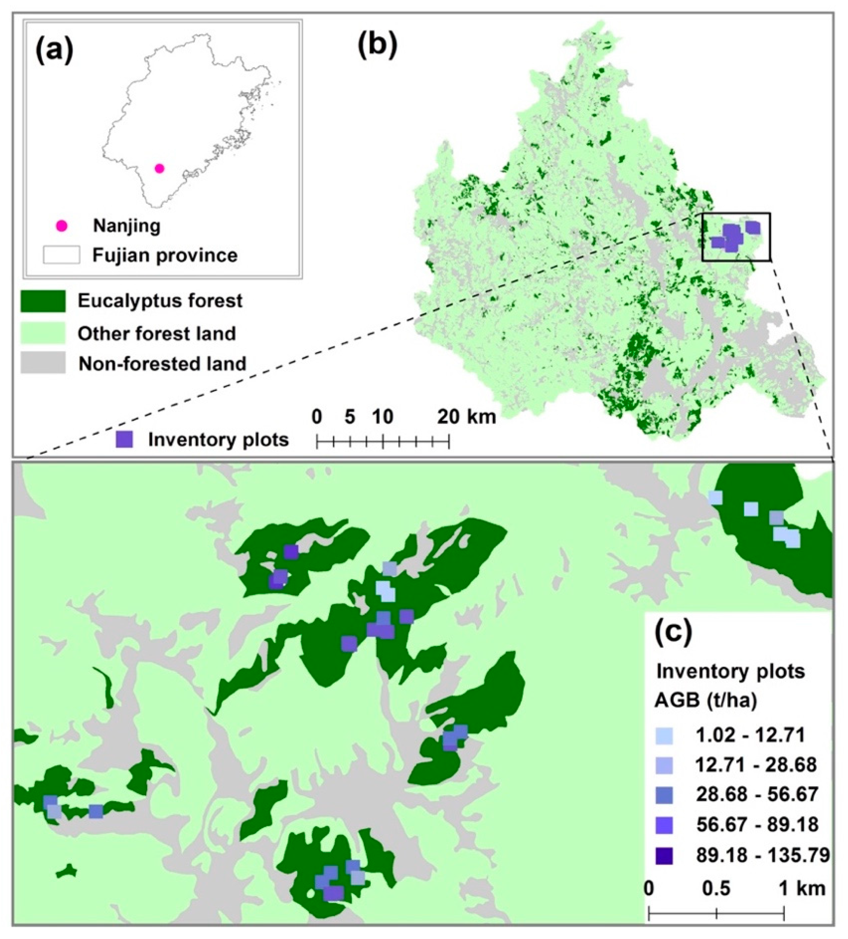
2.1. Study Area

The study area was in Fujian Province, Nanjing County, China (117°00′–117°36′ E, 24°26′–25°00′ N, Figure 1). The region has a South Asian tropical monsoon climate. The average annual temperature in Nanjing County is 21 °C, with an annual precipitation of 1700 mm and 340 frost-free days per year. The major soil type is red soil. The study area has a complex topography with significantly varying elevation (0–1566 m). Seventy-four percent (145,009 ha) of the county comprises forests, and 79,346 ha are plantations. The main tree species are Eucalyptus grandis x urophylla, Pinus massoniana, and Cunninghamia lanceolata (Lamb.) Hook. Forest composition, structure, and biomass are spatiotemporally heterogeneous. Over the past decade, the area of Eucalyptus plantations increased by 10,862 ha, reaching 13,338 ha.

2.2. Reference AGB Data

This dataset contains the reference AGB of all 30 inventory plots in the study area. A total of 30 inventory plots were selected in 2012. The 30 inventory plots included ten Eucalyptus plantation age groups, and each group included three inventory plots. The plots were in the eastern section of the study area (Figure 1). In each plot (0.04 ha, 20 m × 20 m), we measured the diameter at breast height (DBH) and tree height (H) of all living stems. In addition, we investigated the environmental data and forest attributes of inventory plots, including stand age, stand density, longitude, latitude, and altitude.

Table 1. Statistics of inventory plots.

Item	Mean ± Standard Deviation	Median	Range (Minimum, Maximum)
AGB (t/ha)	47.34 ± 34.46	46.64	(1.02, 135.79)
Longitude	117.48 ± 0.02	117.47	(117.446, 117.503)
Latitude	24.71 ± 0.01	24.71	(24.694, 24.721)
Altitude (m)	269.2 ± 82.5	313.5	(135, 389)
Stand density (stems/ha)	852.5 ± 251.8	800.0	(450, 1375)
DBH (cm)	12.29 ± 4.48	13.19	(2.19, 17.99)
H (m)	12.98 ± 4.72	14.42	(2.83, 18.23)
Age (years)	5.5 ± 2.92	5.5	(1, 10)

lists the statistics of the inventory plots.

The AGB of each plot was obtained by summing the AGB of all trees within the plot. The AGB of each tree was estimated using H, DBH, and three allometric models built in this study.

Obtaining reference AGB data involved the following steps: (1) destructive sampling in inventory plots (i.e., tree harvest), (2) construction of tree-level allometric models, and (3) calculation of reference AGB of inventory plots. Details on obtaining reference AGB data are provided in Section A of the Supplementary Material.

2.2.1. Destructive Sampling in Inventory Plots: Tree Harvest

Trees were harvested from the 30 inventory plots. Three trees with a DBH close to the mean DBH of trees in each plot were cut down, for a total of 90 trees harvested from the 30 plots. We then measured the H and DBH of each harvested tree and weighed the biomass of each organ (foliage, stems, and branches) to obtain the AGB of each harvested tree. Details on the selection of the standard wood and cutting process are provided in Section A of the Supplementary Material. Due to environmental impacts, trees of the same forest age may also have different chemical, physical, and energy characteristics that may affect their biomass [23]. To harvest as many representative trees as possible, we harvested three trees per plot.

2.2.2. Construction of Tree-Level Allometric Models

We divided the 90 harvested trees into three age groups (1–2 years, 3–5 years, and 6–10 years) to construct tree-level allometric models:

$$\mathrm{AGB}=\mathrm{a}\times {\left({\left(\mathrm{DBH}\right)}^2\times \mathrm{H}\right)}^{\mathrm{b}},$$

(1)

where a and b are constant coefficients.

Table 2. Parameters used in tree-level allometric models.

Number	Age (Years)	a	b	R2
1	1–2	0.1538	0.6993	0.99
2	3–5	0.0377	0.9244	0.98
3	6–10	0.0689	0.8489	0.88

lists the parameters used in these models.

2.2.3. Calculating Reference AGB of Inventory Plots

The tree-level allometric models (Table 2) were then applied to each tree in each inventory plot according to tree age, DBH, and H. The resulting tree AGB was aggregated on the plot level, thereby producing a reference AGB for each of the 30 inventory plots.

The reference AGB for the 30 inventory plots ranged from 1.02 to 135.79 Mg·ha⁻¹, with an average value of 47.34 Mg·ha⁻¹ and a standard deviation of 34.46 Mg·ha⁻¹. The coefficients of variation of the AGB for all inventory plots and for the ten age categories were 0.73 and 0.07–0.37, respectively.

2.2.4. Spatial Characteristic Test of Forest Reference AGB

The spatial-characteristic test of forest reference AGB is the premise for using the P-BSHADE spatial statistical model. We used the R software to calculate Moran’s I [24] to evaluate the spatial autocorrelation of the reference AGB between inventory plots. Spatially stratified heterogeneity refers to the within-strata variance being less than the between-strata variance. The spatially stratified heterogeneity of the reference AGB was evaluated by using a q-statistic generated by the GeogDetector model. GeogDetector is a software tool that analyzes the spatial variation in the geographic strata (or hierarchical) of variables [25]. First, we used the K-means algorithm to obtain the strata of the reference AGB. Next, we regarded the reference AGB as Y and the strata of the reference AGB as X and inserted them into the GeogDetector model to obtain the q statistics [25,26].

2.3. Selection of Variables

To create the plot-level model, we first identified predictor variables. Based on our previous work [27], we selected environmental covariates, including longitude, latitude, and altitude, and forest attribute variables, including stand density, plot mean DBH, plot mean H, and forest age. Pearson’s correlation coefficient was used to investigate the correlation between these variables and the reference AGB of the inventory plots.

2.4. Model Development

Seven models, including three machine learning models (Figure 2a–c), one spatial statistical model (Figure 2d), and three combined machine learning and spatial statistical models (Figure 2a,d, Figure 2b,d and Figure 2c,d) were developed and trained to predict the AGB of the inventory plots. The three machine learning models included (a) SVM, (b) RBF-ANN, and (c) RF, and the one spatial statistical model was (d) P-BSHADE. The three combined models are denoted SVM & P-BSHADE, RBF-ANN & P-BSHADE, and RF & P-BSHADE.

The spatial statistical model P-BSHADE requires AGB-related variables. In this case study, we used the estimated AGB data of the plots as the AGB-related variables (see “estimated AGB data of plots” in Figure 2). For the combined machine learning and spatial statistical models, the estimated AGB data of the plots were obtained from the results of SVM (Figure 2a), RBF-ANN (Figure 2b), or RF (Figure 2c). For the P-BSHADE model only (Figure 2d), we established a plot-level allometric model to obtain the estimated AGB data of the plots.

The models were trained by using the R Development Core Team.

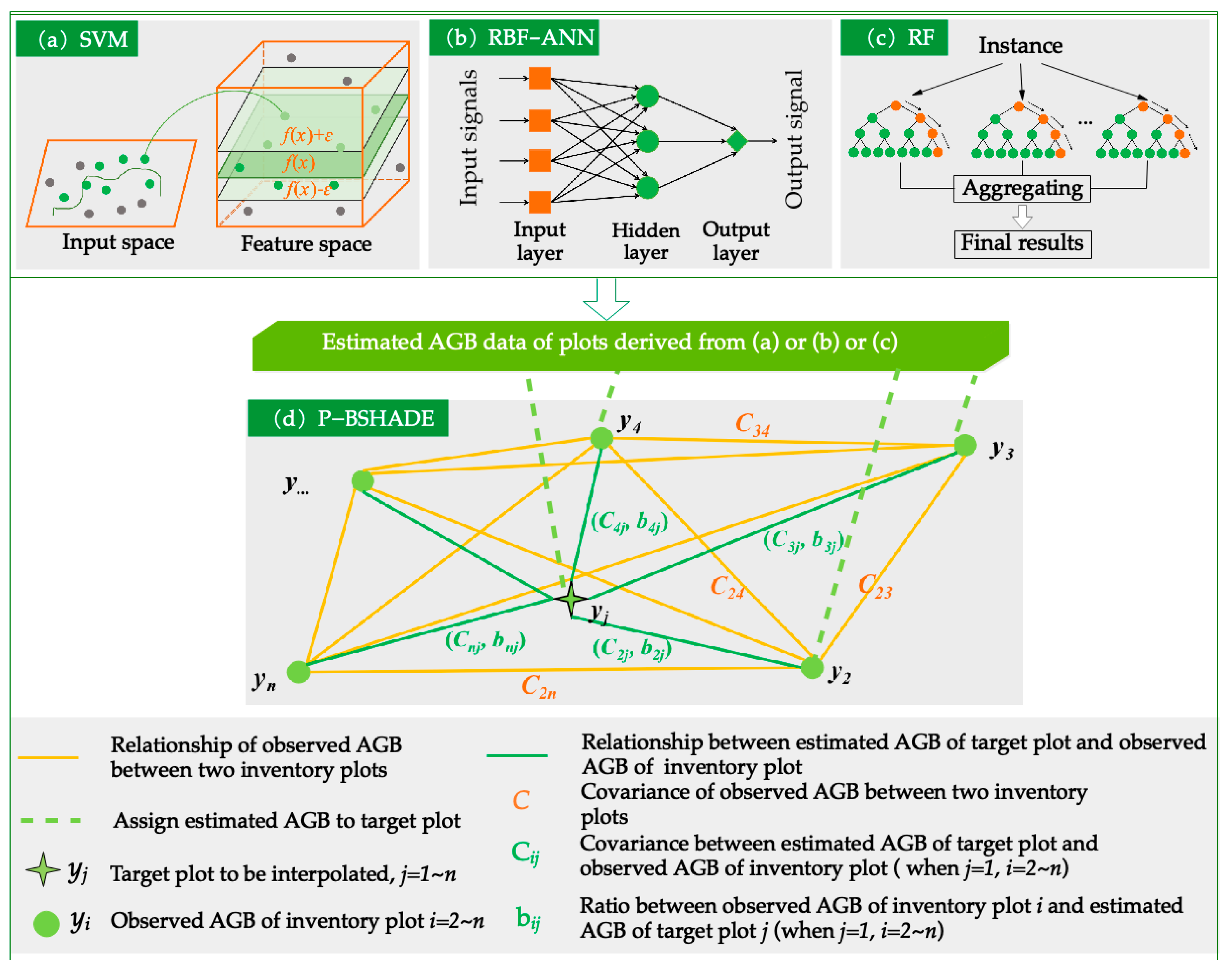
2.4.1. Machine Learning

SVM, RF, and ANN are robust machine learning models for estimating forest biomass and volume, mapping soil organic carbon stocks, and geological mapping [11,28,29,30]. Therefore, we selected SVM, RBF-ANN, and RF machine learning models for this research.

SVM is a method of supervised machine learning that is often used to solve classification problems or regression problems. The basic principle of SVM for classification is to find a hyperplane in the feature space and separate the positive and negative samples with the minimum misclassification rate [31]. The principle of SVM for regression is very similar to that of SVM for classification [32]. SVM for regression retains the main ideas of minimizing error and individualizing the hyperplane that maximizes the margin, and part of the error is acceptable [32].

RBF-ANN is a three-layer neural network model that includes an input layer, a hidden layer (a Gaussian RBF is used here), and an output layer. The transformation from input space to hidden space may be linear or nonlinear, whereas the transformation from hidden space to output space is linear. The function of the hidden layer is to map the vector from the indivisible low-dimensional linear state to the separable high-dimensional linear state to greatly accelerate the learning and convergence speed and avoid becoming stuck in a local optimum [33].

RF is a machine learning technique and data mining method that combines self-learning technologies and was developed by Breiman in 2001 [34]. RF combines tree predictors such that each tree depends on the values of a random vector that is sampled independently and with the same distribution for all trees in the forest. RF provides accurate predictions [34].

The schematic function for machine learning is

$$y_j=f\left(x_{j,1},x_{j,2},x_{j,3},x_{j,4}\right),$$

(2)

where $y_j$ is the AGB of the $j$th inventory plot predicted by a machine learning model $\left(j=1,\dots ,n, n=30\right)$, $f(\dots )$ is a machine learning model represented by a function of $x_{j,k}$ $\left(k=1,\dots ,4\right)$, and $x_{j,1}$, $x_{j,2}$, $x_{j,3}$, and $x_{j,4}$ are the central longitude, mean DBH, mean H, and forest age of the $j$th inventory plot, respectively.

2.4.2. Spatial Statistical Model: P-BSHADE

P-BSHADE is an optimal linear unbiased estimate-interpolation method based on the assumption of the simultaneous existence of the spatial autocorrelation and heterogeneity of the target object. This method is empirically superior for solving the problem of an unrepresentative sample when estimating [35,36].

The core of the model is to minimize the variances between predicted error and unbiased estimation. The prediction process of the P-BSHADE model requires strong spatio-temporal coordination between the predictive variable and the related variable to spatially interpolate the predictive variable.

P-BSHADE differs markedly from the kriging and inverse distance weighting (IDW) algorithms. Compared with kriging and IDW, the application of P-BSHADE to forest AGB interpolation has the following advantages: (1) The spatial distribution of forest AGB is characterized by spatial autocorrelation and heterogeneity, which are taken into account in the P-BSHADE model. Considering spatial heterogeneity eliminates the difference in forest AGB distribution caused by varying terrains or different geographic locations. However, kriging and IDW only consider the spatial correlation between plots. (2) In addition, P-BSHADE considers strongly correlated inventory plots as neighboring plots, whereas the kriging and IDW algorithms consider sites that are close in proximity.

In brief, the P-BSHADE model includes three steps: First, the model obtains reference AGB for all inventory plots by using the allometric model. Second, it uses the reference AGB of the target inventory plot and the reference AGB of other inventory plots to obtain the weight relationship between the target inventory plot and the other inventory plots. Third, it uses the reference AGB of the other inventory plots and weights in Equation (3) to predict the AGB of the inventory plots. The specific mathematical formula for the P-BSHADE model is (see Supplementary Material [35,36])

$${\widehat{y}}_j={\sum }_{i=1}^n{w}_{ij}{y}_i,$$

(3)

where ${\widehat{y}}_j$ is the estimated AGB of the $j$th inventory plot using the P-BSHADE model $\left(j=1, 2, \dots , n, n=30\right)$, $y_i$ is the reference AGB of the $i$th inventory plot $\left(i=1, 2, \dots , n, n=30\right)$, $w_{ij}$ is calculated by dividing the reference AGB of the ith inventory plot by the (allometric model) estimated AGB of the $j$th inventory plot (when $j=1, i=2, 3, \dots , 30$; when $j=2, i=1, 3, 4, \dots , 30$).

2.4.3. Combination of Machine Learning and Spatial Statistical Models

Considering the inherent advantages and disadvantages of P-BSHADE and machine learning, this study investigates whether they can improve the accuracy of forest AGB estimates. Therefore, P-BSHADE was separately integrated with the three machine learning methods (SVM, RBF-ANN, and RF) to form three combined models (SVM & P-BSHADE, RBF-ANN & P-BSHADE, and RF & P-BSHADE). The specific and most important combination step was to use the estimated results from the machine learning models as reference data. Therefore, the equation of each combined model is the same as Equation (3), with the description of $w_{ij}$ replaced by “$w_{ij}$ is calculated by dividing the reference AGB of the $i$th inventory plot by the machine-learning-estimated AGB of the $j$th inventory plot (when $j=1, i=2, 3, \dots , 30$; when $j=2, i=1, 3, 4, \dots , 30$)”.

2.5. Model Evaluation and Comparison

2.5.1. Split Datasets

Considering that the 30 inventory plots were relatively centralized and that spatial autocorrelation of the data was possible, we used a spatial block cross-validation strategy to split datasets to avoid overfitting of the model when using machine learning. The major difference between standard random k-fold cross-validation and spatial block cross-validation is how the datasets are split into folds. Numerous studies have shown that spatial block cross-validation is more suitable than random k-fold cross-validation in the field of ecology when using environmental data because it reduces model overfitting [37,38,39,40]. More information on this topic and an R package of the spatial block k-fold cross-validation are available in [40].

After the spatial block, the 30 inventory plots were split into 12 clusters (see the 12 squares of Figure S1 of the Supplementary Material), and the 12 clusters were then split tenfold to apply tenfold cross-validation (Figure S2 shows one instance of tenfold cross-validation).

2.5.2. Calculate Indicators

To evaluate the accuracy of the AGB estimates of the seven models (SVM, RBF-ANN, RF, P-BSHADE, SVM & P-BSHADE, RBF-ANN & P-BSHADE, and RF & P-BSHADE), the estimated AGB results were compared with the reference AGB of the inventory plots. As performance indicators, we used the mean absolute error (MAE), mean relative error (MRE), root mean square error (RMSE), and normalized root mean square error (nRMSE), which are given by

$$MAE=({\sum }_{i=1}^n\left|y_i^p-y_i\right|)/n,$$

(4)

$$MRE=\left({\sum }_{i=1}^n\frac{\left|y_i^P-y_i\right|}{y_i}\right)/n,$$

(5)

$$RMSE=\sqrt{\left({\sum }_{i=1}^n{\left(y_i^p-y_i\right)}^2\right)/n},$$

(6)

$$nRMSE=\frac{\sqrt{\left({\sum }_{i=1}^n{\left(y_i^p-y_i\right)}^2\right)/n}}{{\overline{y}}_i},$$

(7)

where $y_i^p$ is the predictive value of the different models, $y_i$ is the reference AGB of the $i$th inventory plot, and $n$ is the number of training datasets. We then used the calculated MAE, MRE, and RMSE to identify the optimal model.

2.5.3. Robustness of Combined Models

To evaluate the robustness of the combined machine learning and spatial statistical models for different time series, we selected 22 independent sample plots and made nondestructive measurements of each tree in July 2019. We repeated the process used for constructing the plot-level model and evaluated the models. We then used the accuracy-assessment indexes (MAE, MRE, RMSE, and nRMSE) to determine whether the combined models were more accurate than the single models.

3. Results

3.1. Spatial Characteristic Test of Forest Reference AGB

The spatial autocorrelation test produced a Moran’s I value of 0.36, a z score of 4.78, and a p value less than 0.01 (p < 0.01). The spatial distribution of the reference AGB revealed a pattern of aggregation (see red regions in Figure S3 in the Supplementary Material). Less than 1% of the AGB data were randomly distributed (see blue regions in Figure S3 in the Supplementary Material), and the possibility of an aggregated distribution was greater than that of a random distribution. These results suggest that the spatial distribution of the AGB data reveals aggregation and a pattern of strong spatial autocorrelation.

The spatially stratified heterogeneity test produced a q value of 0.87 and a p value less than 0.01, which indicate that the within-layer variances were far less than the sum of variances between different strata. The results indicate that the reference AGB of the 30 inventory plots can be described by spatially stratified heterogeneity.

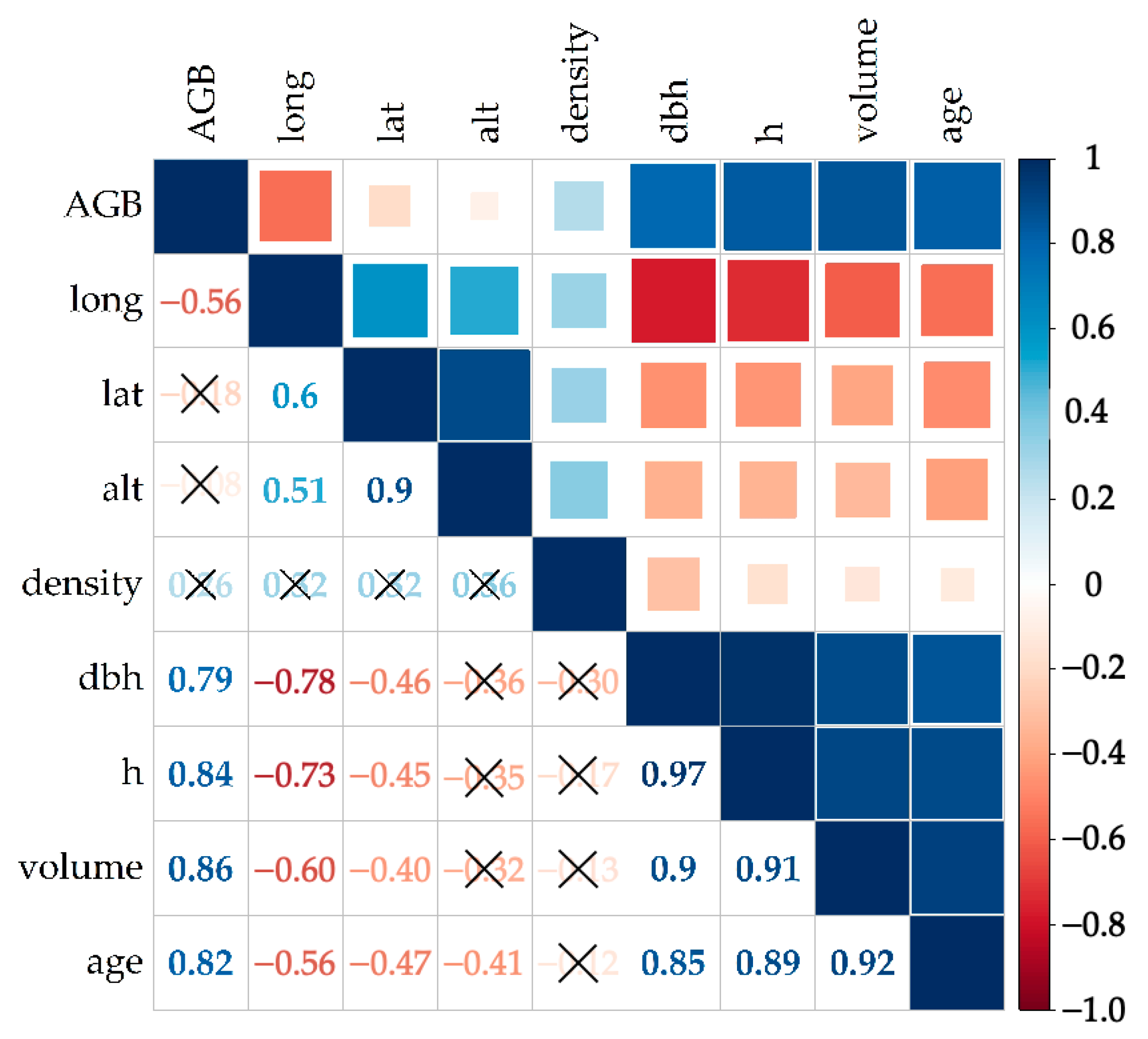
3.2. Selection of Variables

Figure 3 shows the correlation-coefficient matrix of variables. The following variables were strongly correlated with AGB: longitude (r = −0.56), DBH (r = 0.79), H (r = 0.84), and forest age (r = 0.82). Thus, we selected four variables (longitude, DBH, H, and forest age) as covariates for the AGB plot-level models. Table 1 lists the statistical descriptions of these covariates and the AGB statistics for the 30 inventory plots.

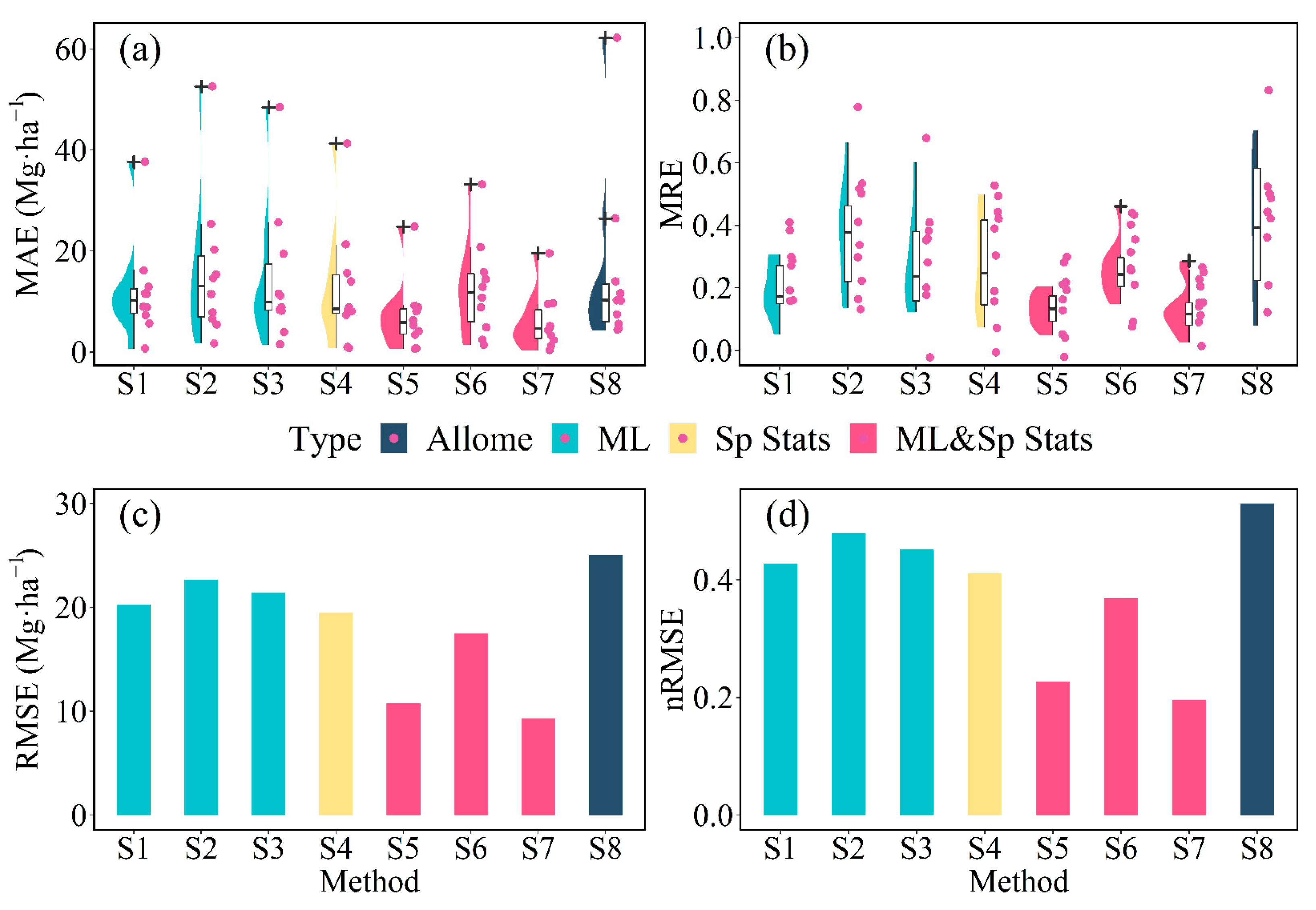
3.3. Performance of Plot-Level Models

An allometric model was applied to compare with our seven models. The indicators of the allometric model are greater than those of the seven models developed in this study (Figure 4). The forest AGB estimates obtained by the P-BSHADE method are similar to those obtained by the three machine learning methods.

Of the three machine learning methods, the SVM was the most accurate. The three evaluation indexes (MAE = 13.66 Mg·ha⁻¹, RMSE = 20.25 Mg·ha⁻¹, and nRMSE = 0.43) were substantially lower than those for the other two machine learning methods (MAE = 15.19–15.35 Mg·ha⁻¹, RMSE = 21.40–22.69 Mg·ha⁻¹, and nRMSE = 0.45–0.48).

The combination of machine learning and spatial statistical models produced smaller MAE (5.89–11.87 Mg·ha⁻¹), MRE (0.13–0.24), RMSE (9.29–17.47 Mg·ha⁻¹), and nRMSE (0.20–0.37) than the single machine learning methods and the P-BSHADE model.

Of the three combined methods, RF & P-BSHADE was the most accurate, with the smallest MAE (5.89 Mg·ha⁻¹), a modest MRE (0.14), and the smallest RMSE (9.29 Mg·ha⁻¹) and nRMSE (0.20). In contrast, RBF-ANN & P-BSHADE produced the highest MAE (11.87 Mg·ha⁻¹), MRE (0.24), RMSE (17.47 Mg·ha⁻¹), and nRMSE (0.37). Compared with the RF model, the RF & P-BSHADE model led to a reduction in the cross-validated prediction error of 56.60–87.43% (61.22% for MAE, 87.43% for MRE, and 56.60% for RMSE and nRMSE, see Figure 4).

We now compare the machine learning methods with combined methods over two periods, 2012 and 2019 (Figure 5). Whether considering the data from 2012 or the new data collected in 2019, the combined model is more accurate than the single machine learning model, although p-values change with the methods and with predictive indicators. (

Table 3. The prediction indicator differs between the three machine learning methods and the combined methods. A paired t-test was used to examine if the predictive indicators (i.e., MAE and RMSE) of the combined methods are greater than those of the machine learning method alone based on the results of the 10-fold cross-validation.

Method	p-Value for MAE		p-Value for MRE		p-Value for RMSE		p-Value for nRMSE
	2012	2019	2012	2019	2012	2019	2012	2019
S1 vs. S5	0.209	0.005 ***	0.289	0.108	0.148	0.009 ***	0.168	0.009 ***
S2 vs. S6	0.525	0.582	0.090 *	0.269	0.588	0.809	0.134	0.817
S3 vs. S7	0.081 *	0.029 **	0.216	0.033 **	0.091 *	0.040 **	0.089 *	0.003 ***

Note: S1 = SVM, S2 = RBF-ANN, S3 = RF, S5 = SVM & P-BSHADE, S6 = RBF-ANN & P-BSHADE, S7 = RF & P-BSHADE * denote 0.1 significant; ** denote 0.05 significant; *** denote 0.01 significant.

). These results suggest that the combined models are more accurate than single machine learning models, and these improvements are robust.

4. Discussion

4.1. Significance and Challenges of Accurate Plot-Level AGB Estimates

Plot-level AGB models link tree-level AGB measurements to regional-scale AGB estimates. Ignoring the uncertainty of plot-level models underestimates the total uncertainty of pixel-level estimates by 6% [2]. In the field of forest biomass estimation, the accurate estimation of forest AGB or structure at the plot level is very important for calibrating and validating large-scale forest biomass. However, the distribution of most AGB is either non-Gaussian, skewed, or multimodal, especially in tropical and subtropical regions [41]. Different intensities and factors are coupled together, resulting in high heterogeneity and clear nonlinearity in the spatial distribution of forest AGB. These spatial characteristics of forest AGB make it more difficult to accurately estimate AGB at the plot level.

Here, we integrate the advantages of machine learning and spatial statistics to construct a plot-level AGB model for a subtropical region. Combining the advantages of machine-learning-based quantification of complex nonlinear relationships between AGB and the multiple covariates, in conjunction with the P-BSHADE model, allows the spatial autocorrelation and heterogeneity of forest AGB to be incorporated into the model.

4.2. Why a Combined Model Outperforms a Single Machine Learning or Spatial Statistical Model

As expected, the combined methods were more accurate than any single method (either machine learning or spatial statistics). This may be due to the advantages of machine learning, which compensates for the inherent defects of the P-BSHADE model, and vice versa.

On the one hand, the P-BSHADE model has its own merits: (1) It considers the spatial autocorrelation and spatial heterogeneity of the distribution of the target objects, not only to solve the difference between target objects caused by the different terrain or geographic location but also to solve the problem of strong correlation between target objects with remote geographic locations due to similar terrain conditions. (2) The P-BSHADE model calculates the covariance of the reference data of research objects, that is, the reference AGB of inventory plots in our study. This method is more reliable because it avoids the second-order stationary hypothesis (i.e., when using the kriging algorithm, semivariograms require this hypothesis), which does not correspond with the actual situation. (3) P-BSHADE regards strongly correlated plots as neighboring plots. However, the P-BSHADE model is also handicapped by the fact that the founding assumption does not conform to reality. The assumption is that the estimated AGB is accurate in all inventory plots except in the target inventory plot. In other words, the premise behind using the P-BSHADE model is that the reference AGB data are accurate or strongly correlated with AGB. In reality, the AGB of each inventory plot has a varying degree of uncertainty when using the single P-BSHADE model because the reference AGB data were obtained from the allometric model. As the P-BSHADE model combined with machine learning uses the results optimized by machine learning as the reference AGB data, it further improves the accuracy of AGB mapping.

On the other hand, machine learning also has advantages and disadvantages. Machine learning has the advantage of being able to handle complex, potentially nonlinear relationships between forest AGB and other variables. However, the initial samples of machine learning are randomly selected, which may lead to differences in the results of each operation of the model. In addition, one of the important shortcomings is overfitting, which may perform poorly beyond the training data range. In contrast with machine learning, the P-BSHADE model considers the spatial autocorrelation and spatial heterogeneity of forest AGB and of environmental covariates and the bias of the observed values of the inventory plots, which better corresponds to actual situations. A combined model uses the results of machine learning as the reference AGB data of P-BSHADE, so that the fitting process of the combined model better accounts for spatial relationships than does the single machine learning model. The result is improved accuracy.

Machine learning models or the P-BSHADE model have been used to model the uncertainty of temperature measurements obtained by weather stations [20,29,36]. However, the methods used in these studies were adopted independently. Conversely, the combination of machine learning and spatial statistics can improve the prediction accuracy of AGB maps, which in turn can be used as criteria for improving the accuracy of LiDAR remote-sensing technology and the results of ecological process models. Eventually, these improvements can promote process-oriented projects that require dynamic AGB predictions for large-scale forests in different forest management scenarios.

Our combined methods produce a very small RMSE for the prediction accuracy of AGB, which we explain as follows: (1) The reference AGB of the 30 inventory plots were obtained by summing the AGB of each tree, which was calculated using allometric models constructed from accurate measurements of harvested trees. (2) Machine learning methods were used to quantify the complex nonlinear relationship between AGB and multiple environmental covariates. (3) We applied a spatial statistical method based on the hypothesis of spatial heterogeneity. Although the nRMSE index is calculated in different studies using different datasets and prediction methods in different locations, most studies use nRMSE as an indicator for quantifying the AGB prediction errors of models [5,6,9]. In contrast with other studies, the present work not only focuses on subtropical forests but also uses methodological differences to mitigate uncertainty, especially by comprehensively addressing the sources of uncertainty caused by multiple spatial and environmental covariates.

4.3. Why the RF & P-BSHADE Method Outperforms Other Combined Methods

The three combined machine learning and spatial statistical methods produced more accurate AGB predictions than any individual method. The RF & P-BSHADE and SVM & P-BSHADE methods were significantly more accurate than the individual methods, whereas the RBF-ANN & P-BSHADE method was only slightly more accurate. The accuracies of the combined methods depend on the accuracy of the reference AGB data (machine-learning-predicted results) [36]. The combined method adds spatial information based on machine learning. In other words, more accurate predicted machine learning results lead to a greater accuracy of the combined method. This is an important scientific contribution of this work; namely, that combining machine learning and spatial statistics improves the accuracy of forest AGB estimation. Therefore, the different improvements offered by the three combined methods may be attributed to the following two mechanisms: (1) The RF has superior properties, and SVM models are easier to use and optimize than RBF-ANN [42]. The number of training samples determines the number of nodes in the hidden layer of the RBF-ANN model, and the number of nodes significantly affects the prediction accuracy. With only 30 training samples used in this study, the combined RBF-ANN & P-BSHADE approach did not significantly improve the prediction accuracy. (2) RBF-ANN is more suitable for nonlinear stochastic dynamic systems [33], whereas the relationship between AGB and environmental covariates in this study is likely a monotonically increasing function.

5. Conclusions

Forest AGB estimates at the plot level play a major role in connecting accurate single-tree AGB measurements to relatively difficult regional AGB estimates. However, AGB estimates at the plot level are plagued by numerous uncertainties. Improving the plot-level model of forest AGB is a key issue in producing accurate AGB maps. A variety of prediction models have been applied to make accurate AGB estimates, all of which have their own advantages and disadvantages. Different approaches complement the advantages of different models and may yield more accurate AGB estimates than would otherwise be produced by using a single method. The main goal of the current study was to determine whether combining machine learning with spatial statistics can improve plot-level AGB estimates.

This study explores the prediction performance of different AGB models, and the results show that the model combining the random forest and P-BSHADE models substantially improves the accuracy of the estimates of forest AGB. The results of this study suggest that combining machine learning with spatial statistics improves plot-level AGB estimates. The understanding gained here should help to improve AGB mapping in other regions and in different types of forests.

References

1. Bustamante, M.M.C.; Roitman, I.; Aide, T.M.; Alencar, A.; Anderson, L.O.; Aragão, L.; Asner, G.P.; Barlow, J.; Berenguer, E.; Chambers, J.; et al. Toward an integrated monitoring framework to assess the effects of tropical forest degradation and recovery on carbon stocks and biodiversity. Glob. Chang. Biol. 2015, 22, 92–109. [Google Scholar] [CrossRef]
2. Chen, Q.; Laurin, G.V.; Valentini, R. Uncertainty of remotely sensed aboveground biomass over an African tropical forest: Propagating errors from trees to plots to pixels. Remote Sens. Environ. 2015, 160, 134–143. [Google Scholar] [CrossRef]
3. Sileshi, G.W. A critical review of forest biomass estimation models, common mistakes and corrective measures. For. Ecol. Manag. 2014, 329, 237–254. [Google Scholar] [CrossRef]
4. Mauya, E.W.; Ene, L.T.; Bollandsås, O.M.; Gobakken, T.; Naesset, E.; Malimbwi, R.E.; Zahabu, E. Modelling aboveground forest biomass using airborne laser scanner data in the miombo woodlands of Tanzania. Carbon Balance Manag. 2015, 10, 28. [Google Scholar] [CrossRef] [PubMed] [Green Version]
5. Gleason, C.J.; Im, J. Forest biomass estimation from airborne LiDAR data using machine learning approaches. Remote Sens. Environ. 2012, 125, 80–91. [Google Scholar] [CrossRef]
6. Benítez, F.L.; Anderson, L.O.; Formaggio, A.R. Evaluation of geostatistical techniques to estimate the spatial distribution of aboveground biomass in the Amazon rainforest using high-resolution remote sensing data. Acta Amaz. 2016, 46, 151–160. [Google Scholar] [CrossRef] [Green Version]
7. Propastin, P. Modifying geographically weighted regression for estimating aboveground biomass in tropical rainforests by multispectral remote sensing data. Int. J. Appl. Earth Obs. Geoinf. 2012, 18, 82–90. [Google Scholar] [CrossRef]
8. Van Der Laan, C.; Verweij, P.; Quiñones, M.J.; Faaij, A.P. Analysis of biophysical and anthropogenic variables and their relation to the regional spatial variation of aboveground biomass illustrated for North and East Kalimantan, Borneo. Carbon Balance Manag. 2014, 9, 8. [Google Scholar] [CrossRef] [PubMed] [Green Version]
9. Babcock, C.; Finley, A.O.; Bradford, J.B.; Kolka, R.; Birdsey, R.; Ryan, M.G. LiDAR based prediction of forest biomass using hierarchical models with spatially varying coefficients. Remote Sens. Environ. 2015, 169, 113–127. [Google Scholar] [CrossRef] [Green Version]
10. Babcock, C.; Finley, A.O.; Cook, B.D.; Weiskittel, A.; Woodall, C.W. Modeling forest biomass and growth: Coupling long-term inventory and LiDAR data. Remote Sens. Environ. 2016, 182, 1–12. [Google Scholar] [CrossRef] [Green Version]
11. Gorgens, E.; Montaghi, A.; Rodriguez, L.C. A performance comparison of machine learning methods to estimate the fast-growing forest plantation yield based on laser scanning metrics. Comput. Electron. Agric. 2015, 116, 221–227. [Google Scholar] [CrossRef]
12. Zhao, K.; Popescu, S.; Meng, X.; Pang, Y.; Agca, M. Characterizing forest canopy structure with lidar composite metrics and machine learning. Remote Sens. Environ. 2011, 115, 1978–1996. [Google Scholar] [CrossRef]
13. Russell, S.; Norvig, P. Artificial Intelligence: A Modern Approach, 3rd ed.; Pearson Education Limited: London, UK, 2016. [Google Scholar]
14. Frey, U.J.; Klein, M.; Deissenroth, M. Modelling complex investment decisions in Germany for renewables with different machine learning algorithms. Environ. Model. Softw. 2019, 118, 61–75. [Google Scholar] [CrossRef]
15. Du, H.; Zhou, G.; Fan, W.; Ge, H.; Xu, X.; Shi, Y.; Fan, W. Spatial heterogeneity and carbon contribution of aboveground biomass of moso bamboo by using geostatistical theory. Plant Ecol. 2009, 207, 131–139. [Google Scholar] [CrossRef]
16. Viana, H.; Aranha, J.; Lopes, D.; Cohen, W.B. Estimation of crown biomass of Pinus pinaster stands and shrubland above-ground biomass using forest inventory data, remotely sensed imagery and spatial prediction models. Ecol. Model. 2012, 226, 22–35. [Google Scholar] [CrossRef]
17. Mitchard, E.T.A.; Feldpausch, T.R.; Brienen, R.J.W.; Lopez-Gonzalez, G.; Monteagudo, A.; Baker, T.R.; Lewis, S.L.; Lloyd, J.; Quesada, C.A.; Gloor, M.; et al. Markedly divergent estimates of A mazon forest carbon density from ground plots and satellites. Glob. Ecol. Biogeogr. 2014, 23, 935–946. [Google Scholar] [CrossRef] [PubMed]
18. Hengl, T.; Heuvelink, G.B.; Stein, A. A generic framework for spatial prediction of soil variables based on regression-kriging. Geoderma 2004, 120, 75–93. [Google Scholar] [CrossRef] [Green Version]
19. Schabenberger, O.; Gotway, C.A. Statistical Methods for Spatial Data Analysis; Chapman & Hall0CRC: Boca Raton, FL, USA, 2005. [Google Scholar]
20. Paul, K.I.; Roxburgh, S.H.; Chave, J.; England, J.; Zerihun, A.; Specht, A.; Lewis, T.; Bennett, L.; Baker, T.G.; Adams, M.; et al. Testing the generality of above-ground biomass allometry across plant functional types at the continent scale. Glob. Chang. Biol. 2016, 22, 2106–2124. [Google Scholar] [CrossRef]
21. Saatchi, S.S.; Harris, N.L.; Brown, S.; Lefsky, M.; Mitchard, E.T.A.; Salas, W.; Zutta, B.R.; Buermann, W.; Lewis, S.L.; Hagen, S.; et al. Benchmark map of forest carbon stocks in tropical regions across three continents. Proc. Natl. Acad. Sci. USA 2011, 108, 9899–9904. [Google Scholar] [CrossRef] [PubMed] [Green Version]
22. Zheng, D.; Rademacher, J.; Chen, J.; Crow, T.; Bresee, M.; Le Moine, J.; Ryu, S.-R. Estimating aboveground biomass using Landsat 7 ETM+ data across a managed landscape in northern Wisconsin, USA. Remote Sens. Environ. 2004, 93, 402–411. [Google Scholar] [CrossRef]
23. Roman, K.; Barwicki, J.; Rzodkiewicz, W.; Dawidowski, M. Evaluation of Mechanical and Energetic Properties of the Forest Residues Shredded Chips during Briquetting Process. Energies 2021, 14, 3270. [Google Scholar] [CrossRef]
24. Cliff, A.; Ord, V.J. Spatial Processes: Model and Applications; Pion Ltd.: London, UK, 1981. [Google Scholar]
25. Wang, J.F.; Li, X.H.; Christakos, G.; Liao, Y.L.; Zhang, T.; Gu, X.; Zheng, X.Y. Geographical detectors-based health risk assessment and its application in the neural tube defects study of the Heshun region, China. Int. J. Geogr. Inf. Sci. 2010, 24, 107–127. [Google Scholar] [CrossRef]
26. Wang, J.F.; Zhang, T.L.; Fu, B.J. A measure of spatial stratified heterogeneity. Ecol. Indic. 2016, 67, 250–256. [Google Scholar] [CrossRef]
27. Ren, Y.; Zhang, C.; Zuo, S.; Li, Z. Scaling up of biomass simulation for Eucalyptus plantations based on landsenses ecology. Int. J. Sustain. Dev. World Ecol. 2017, 24, 135–148. [Google Scholar] [CrossRef]
28. Cracknell, M.; Reading, A. Geological mapping using remote sensing data: A comparison of five machine learning algorithms, their response to variations in the spatial distribution of training data and the use of explicit spatial information. Comput. Geosci. 2014, 63, 22–33. [Google Scholar] [CrossRef] [Green Version]
29. Fassnacht, F.; Hartig, F.; Latifi, H.; Berger, C.; Hernández, J.; Corvalán, P.; Koch, B. Importance of sample size, data type and prediction method for remote sensing-based estimations of aboveground forest biomass. Remote Sens. Environ. 2014, 154, 102–114. [Google Scholar] [CrossRef]
30. Were, K.; Bui, D.T.; Dick, Ø.B.; Singh, B.R. A comparative assessment of support vector regression, artificial neural networks, and random forests for predicting and mapping soil organic carbon stocks across an Afromontane landscape. Ecol. Indic. 2015, 52, 394–403. [Google Scholar] [CrossRef]
31. Hearst, M.A.; Dumais, S.T.; Osuna, E.; Platt, J.; Scholkopf, B. Support vector machines. IEEE Intell. Syst. Appl. 1998, 13, 18–28. [Google Scholar] [CrossRef] [Green Version]
32. Sayad, S. Support Vector Machine-Regression (SVR). Available online: https://www.saedsayad.com/support_vector_machine_reg.htm (accessed on 28 November 2021).
33. Elanayar, V.T.S.; Shin, Y. Radial basis function neural network for approximation and estimation of nonlinear stochastic dynamic systems. IEEE Trans. Neural Netw. 1994, 5, 594–603. [Google Scholar] [CrossRef] [Green Version]
34. Breiman, L. Random forests. Mach. Learn. 2001, 45, 5–32. [Google Scholar] [CrossRef] [Green Version]
35. Hu, M.-G.; Wang, J.-F.; Zhao, Y.; Jia, L. A B-SHADE based best linear unbiased estimation tool for biased samples. Environ. Model. Softw. 2013, 48, 93–97. [Google Scholar] [CrossRef]
36. Xu, C.-D.; Wang, J.; Hu, M.; Li, Q. Interpolation of Missing Temperature Data at Meteorological Stations Using P-BSHADE*. J. Clim. 2013, 26, 7452–7463. [Google Scholar] [CrossRef]
37. Meyer, H.; Reudenbach, C.; Wöllauer, S.; Nauss, T. Importance of spatial predictor variable selection in machine learning applications –Moving from data reproduction to spatial prediction. Ecol. Model. 2019, 411, 108815. [Google Scholar] [CrossRef] [Green Version]
38. Pohjankukka, J.; Pahikkala, T.; Nevalainen, P.; Heikkonen, J. Estimating the prediction performance of spatial models via spatial k-fold cross validation. Int. J. Geogr. Inf. Sci. 2017, 31, 2001–2019. [Google Scholar] [CrossRef]
39. Roberts, D.R.; Bahn, V.; Ciuti, S.; Boyce, M.; Elith, J.; Guillera-Arroita, G.; Hauenstein, S.; Lahoz-Monfort, J.J.; Schroder, B.; Thuiller, W.; et al. Cross-validation strategies for data with temporal, spatial, hierarchical, or phylogenetic structure. Ecography 2017, 40, 913–929. [Google Scholar] [CrossRef]
40. Valavi, R.; Elith, J.; Lahoz-Monfort, J.J.; Guillera-Arroita, G. blockCV: An r package for generating spatially or environmentally separated folds for k -fold cross-validation of species distribution models. Methods Ecol. Evol. 2019, 10, 225–232. [Google Scholar] [CrossRef] [Green Version]
41. Marvin, D.C.; Asner, G.; Knapp, D.E.; Anderson, C.; Martin, R.E.; Sinca, F.; Tupayachi, R. Amazonian landscapes and the bias in field studies of forest structure and biomass. Proc. Natl. Acad. Sci. USA 2014, 111, E5224–E5232. [Google Scholar] [CrossRef] [PubMed] [Green Version]
42. Probst, P.; Wright, M.N.; Boulesteix, A. Hyperparameters and tuning strategies for random forest. Wiley Interdiscip. Rev. Data Min. Knowl. Discov. 2019, 9, 1301. [Google Scholar] [CrossRef] [Green Version]
Figure 1. Study area, Eucalyptus plantations, and inventory plots. (a) Geographic location of the study area. (b) Spatial distribution of Eucalyptus plantations (green) and other land-use types. (c) Spatial distribution of the 30 inventory plots used in this study (blue).
Forests 12 01663 g001
Figure 2. Framework for estimating (ac) the machine learning models, (d) the P-BSHADE model, and the three models that combine machine learning with the P-BSHADE model ((a,d), (b,d) and (c,d)).
Forests 12 01663 g002
Figure 3. Pearson’s correlation coefficients between AGB and other variables represented by numbers and squares. Negative (red) numbers indicate that the corresponding variables are negatively correlated, whereas positive (blue) numbers represent positive correlations. Larger absolute numbers are indicated by darker colors, larger squares indicate stronger correlations, and the symbol “×” indicates insignificant correlations.
Forests 12 01663 g003
Figure 4. Prediction performance of the seven different models. (a) MAE and (b) MRE are presented as boxplots for each prediction method, with the median (black horizontal line in the box), interquartile range (25–75% in the box), range 5–95% (whiskers), and outliers (asterisks) labeled (S1 = SVM, S2 = RBF-ANN, S3 = RF, S4 = P-BSHADE, S5 = SVM & P-BSHADE, S6 = RBF-ANN & P-BSHADE, S7 = RF & P-BSHADE, S8 = allometric model, Allome = allometric model, ML = machine learning, and Sp Stats = spatial statistics). Histogram distributions of RMSE and nRMSE for each prediction method are presented in panels (c) and (d), respectively.
Forests 12 01663 g004
Figure 5. Improved accuracy assessment indexes of three combined machine learning and spatial statistical methods are revealed by comparison with three corresponding machine learning methods. Panels (ad) show the MAE, MRE, RMSE, and nRMSE, respectively; S1 vs. S5 compares S5 with S1, S2 vs. S6 compares S6 with S2, and S3 vs. S7 compares S7 with S3 (S1 = SVM, S2 = RBF-ANN, S3 = RF, S5 = SVM & P-BSHADE, S6 = RBF-ANN & P-BSHADE, S7 = RF & P-BSHADE).
Forests 12 01663 g005