Appendix A.2. Individual Polygon Clustering
Our aim was to evaluate which
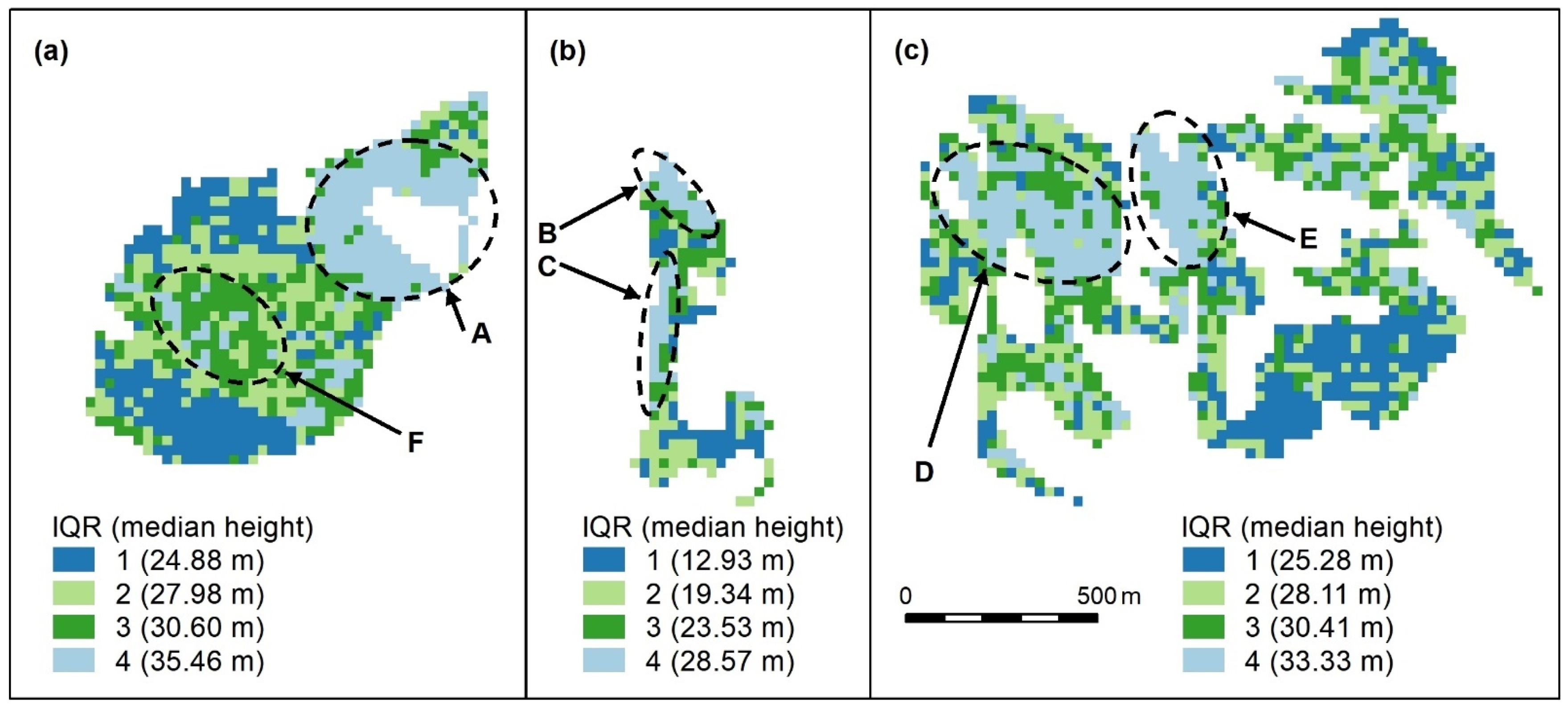
Geoda algorithm best detects higher canopy areas (features A–F) in each of the three polygons depicted in
Figure 12, reproduced below (
Figure A1). The algorithms for the individual polygon groups used only the height data within that group.
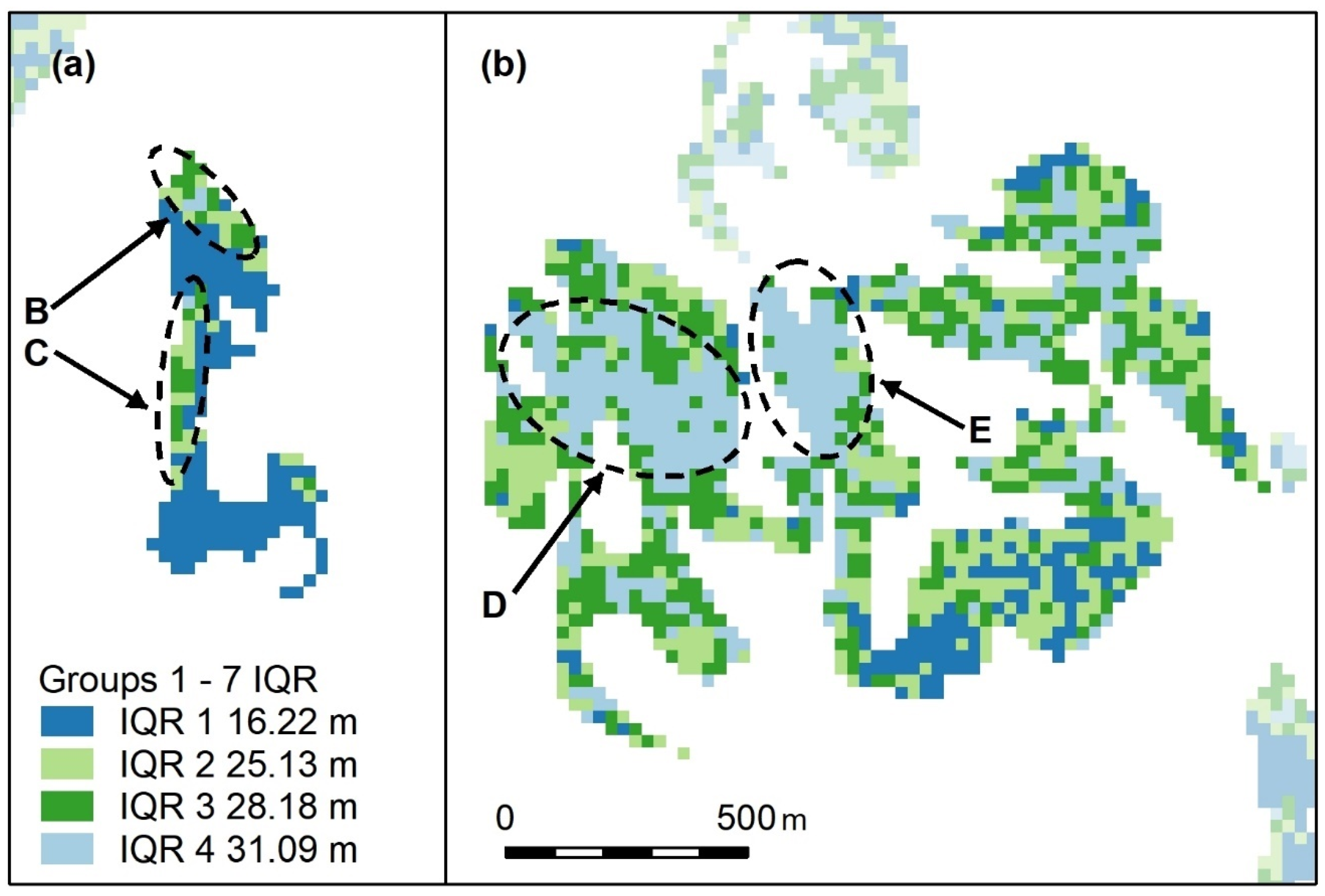
Figure A1.
Compact (a), linear (b), and complex (c) polygon groups, showing the interquartile ranges (IQR) and interquartile median canopy heights within each group. We used this map to assess and compare the clustering algorithm outputs which follow. Spatial patterns are evident, for, e.g., patches of the highest canopy (A–E, light blue) and an area of moderate height (F, dark green), surrounded by a canopy with a slightly lower height (light green). The height appears more randomly distributed in other areas, except for lower canopy height areas (dark blue). All maps use the same scale.
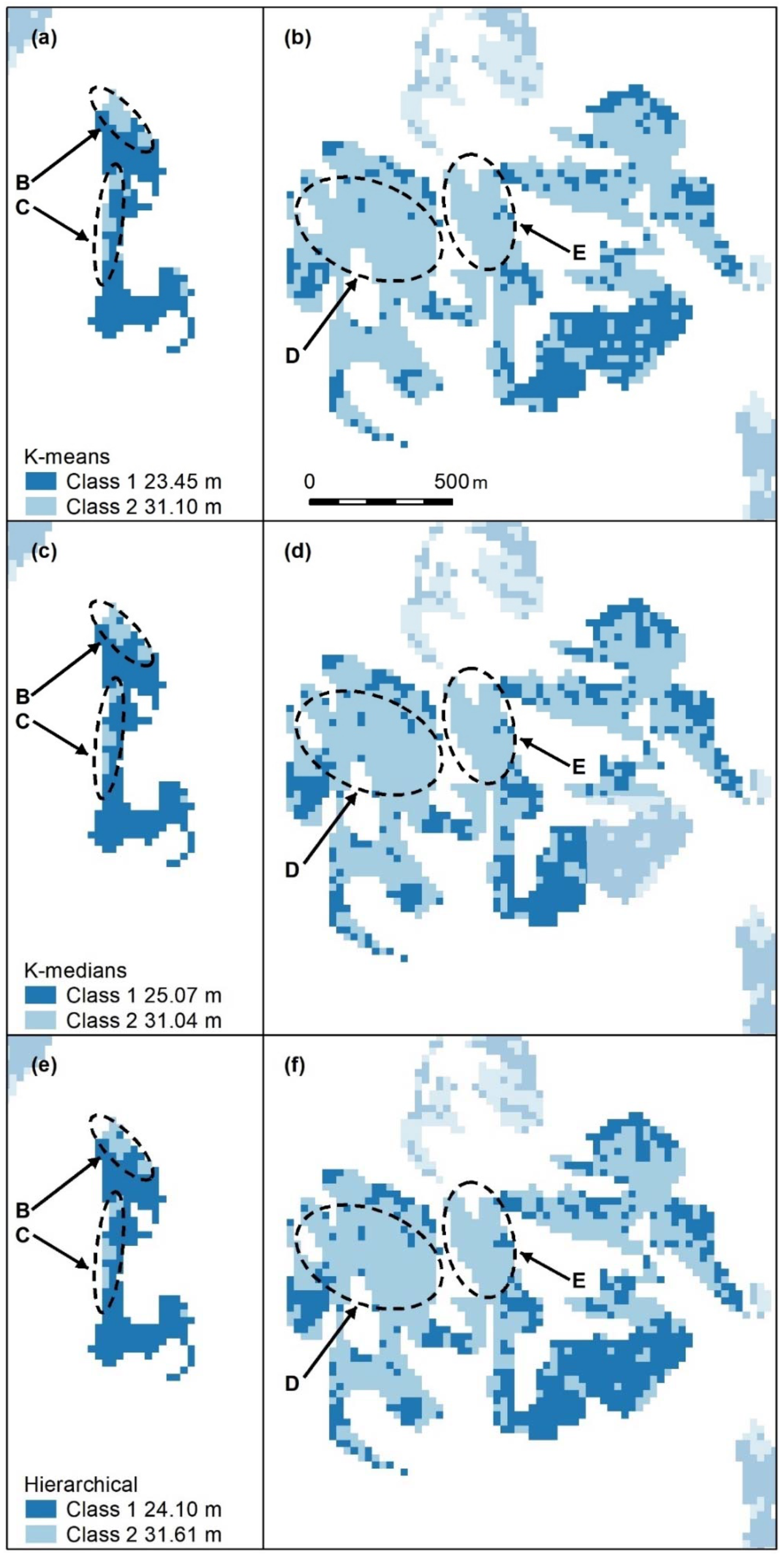
Figure A2.
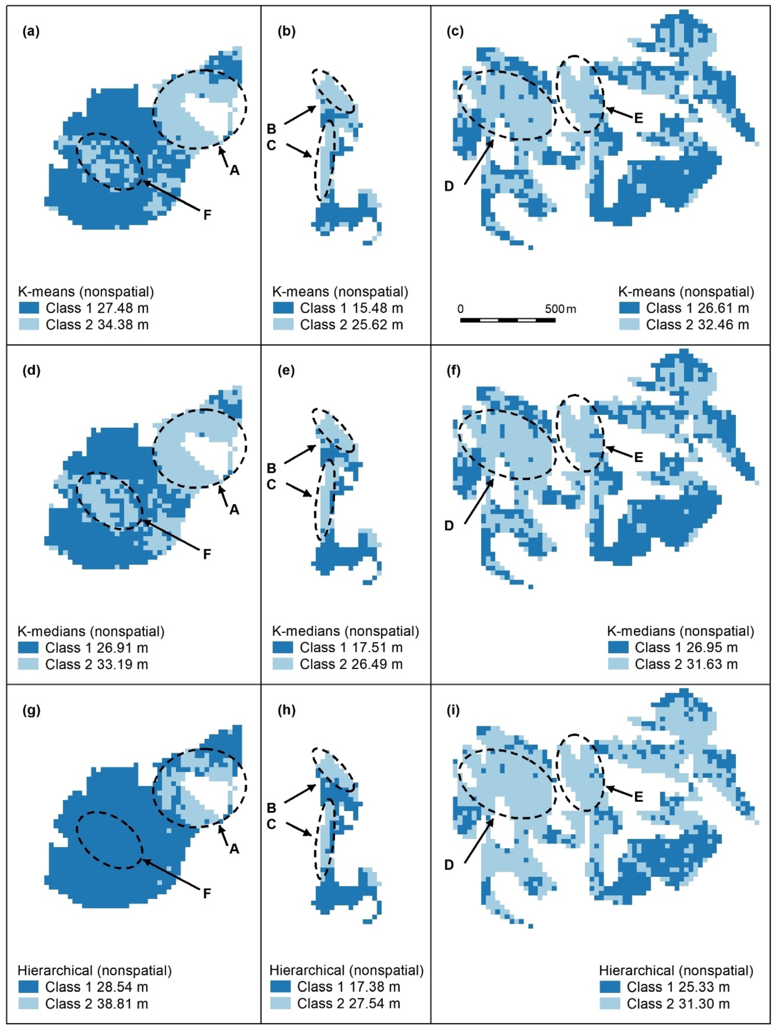
Nonspatial algorithms with 2 classes, using K-means (a–c), K-medians (d–f) and nonspatial hierarchical clustering (g–i). Letters A–F indicate areas of higher canopy. features A–E are captured. K-medians best captures the areal extent of these features and best captures F, an unmapped area of the koala food tree Eucalyptus tereticornis (d). Panel scores: K-means = 16, K-medians = 17, and Hierarchical = 12.
Figure A2.
Nonspatial algorithms with 2 classes, using K-means (a–c), K-medians (d–f) and nonspatial hierarchical clustering (g–i). Letters A–F indicate areas of higher canopy. features A–E are captured. K-medians best captures the areal extent of these features and best captures F, an unmapped area of the koala food tree Eucalyptus tereticornis (d). Panel scores: K-means = 16, K-medians = 17, and Hierarchical = 12.
Figure A3.
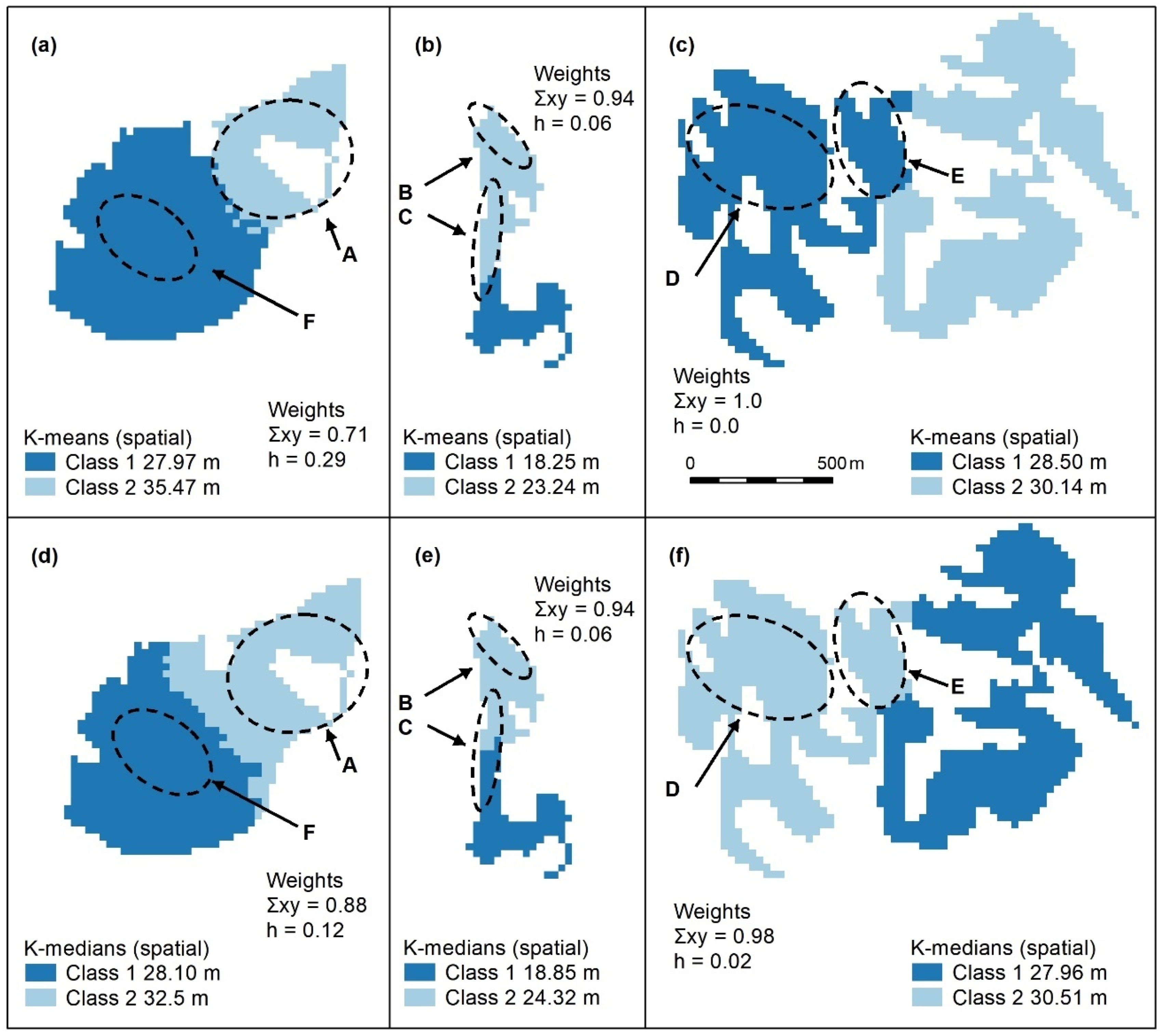
Spatially constrained K-means (a–c) and K-medians (d–f) with 2 classes. These algorithms use spatial weights (x, y), which, in all cases, outweigh those of the object (h = height). Letters A–F indicate areas of higher canopy, only one of the designated features (E) is adequately captured using these algorithms (f). Panel scores: K-means = 6 and K-medians = 8.
Figure A3.
Spatially constrained K-means (a–c) and K-medians (d–f) with 2 classes. These algorithms use spatial weights (x, y), which, in all cases, outweigh those of the object (h = height). Letters A–F indicate areas of higher canopy, only one of the designated features (E) is adequately captured using these algorithms (f). Panel scores: K-means = 6 and K-medians = 8.
Figure A4.
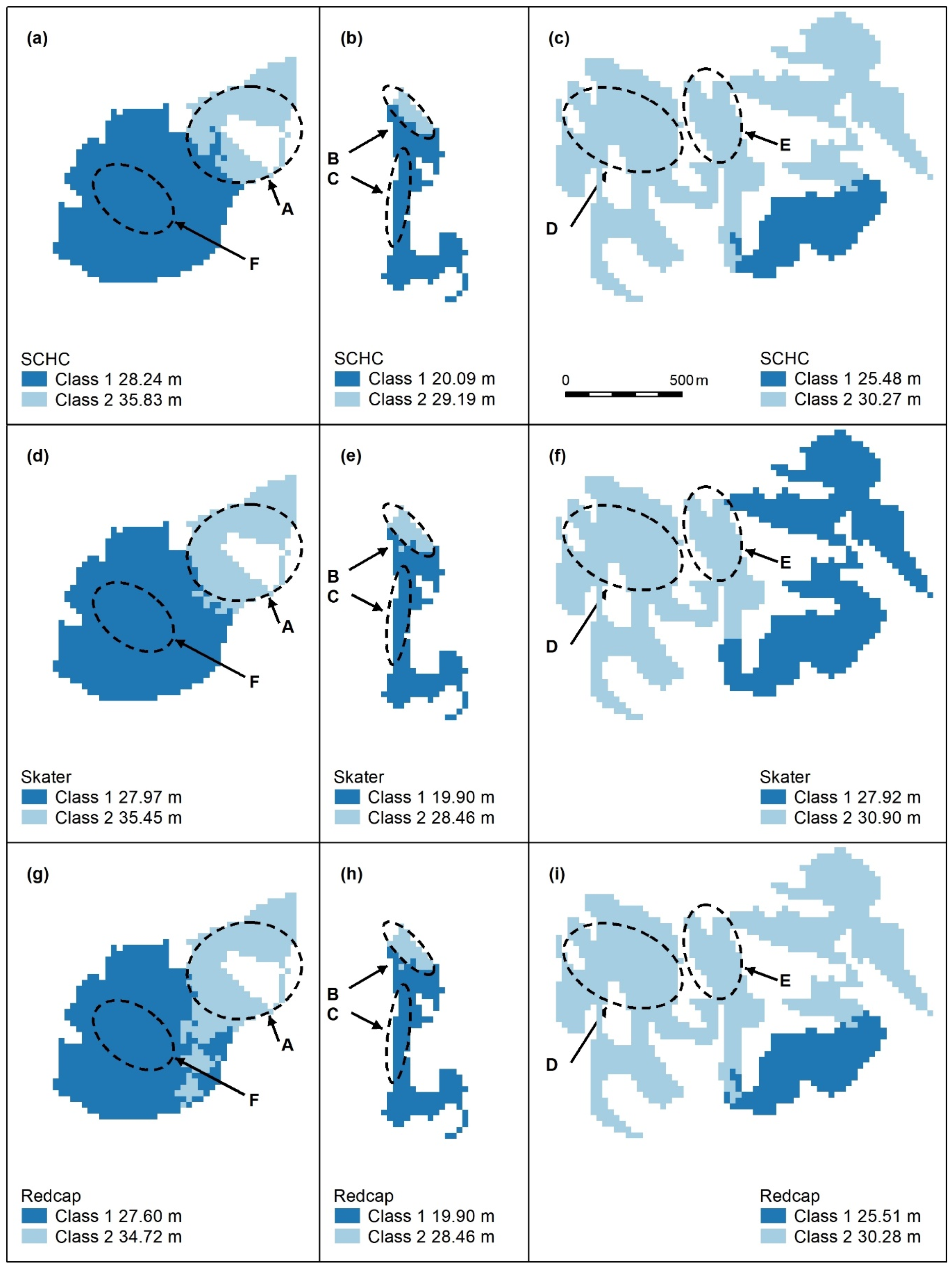
Spatially constrained hierarchical (SCHC, (a–c), Skater (d–f), and Redcap (g–i)) clustering maps with 2 classes. Letters A–F indicate areas of higher canopy, features A and B are adequately captured by these algorithms (a,b,d,e,g,h), but the areal extents of D and E (e,f,i) are too large. C and F are not recognised. Redcap separates an area of regrowth forest on land previously used for farming (g, dark blue) adjoining a relatively undisturbed national park (light blue), which encompasses Feature A. Panel scores: Hierarchical clustering = 9, Skater = 9, and Redcap = 9.
Figure A4.
Spatially constrained hierarchical (SCHC, (a–c), Skater (d–f), and Redcap (g–i)) clustering maps with 2 classes. Letters A–F indicate areas of higher canopy, features A and B are adequately captured by these algorithms (a,b,d,e,g,h), but the areal extents of D and E (e,f,i) are too large. C and F are not recognised. Redcap separates an area of regrowth forest on land previously used for farming (g, dark blue) adjoining a relatively undisturbed national park (light blue), which encompasses Feature A. Panel scores: Hierarchical clustering = 9, Skater = 9, and Redcap = 9.
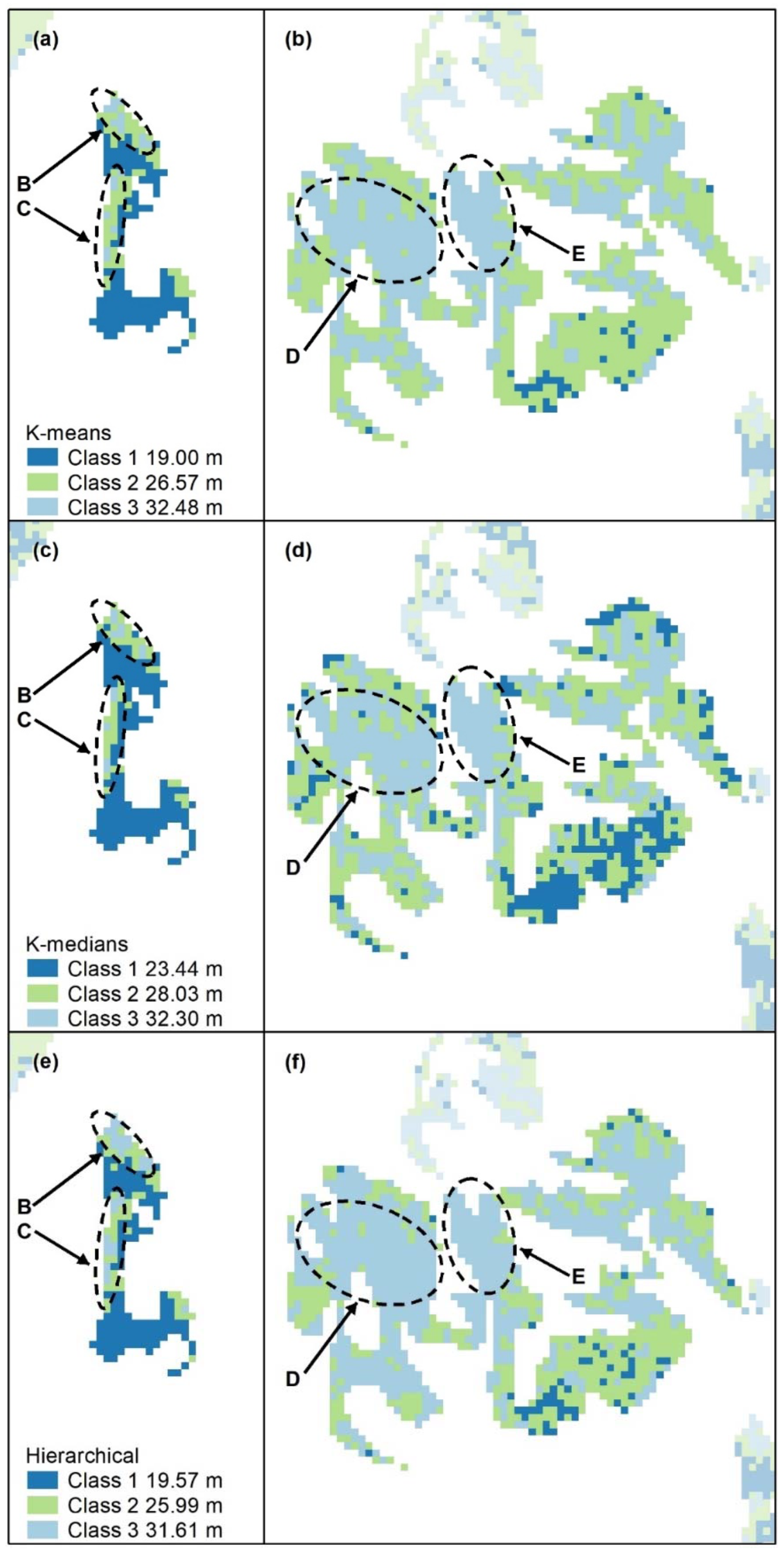
Figure A5.
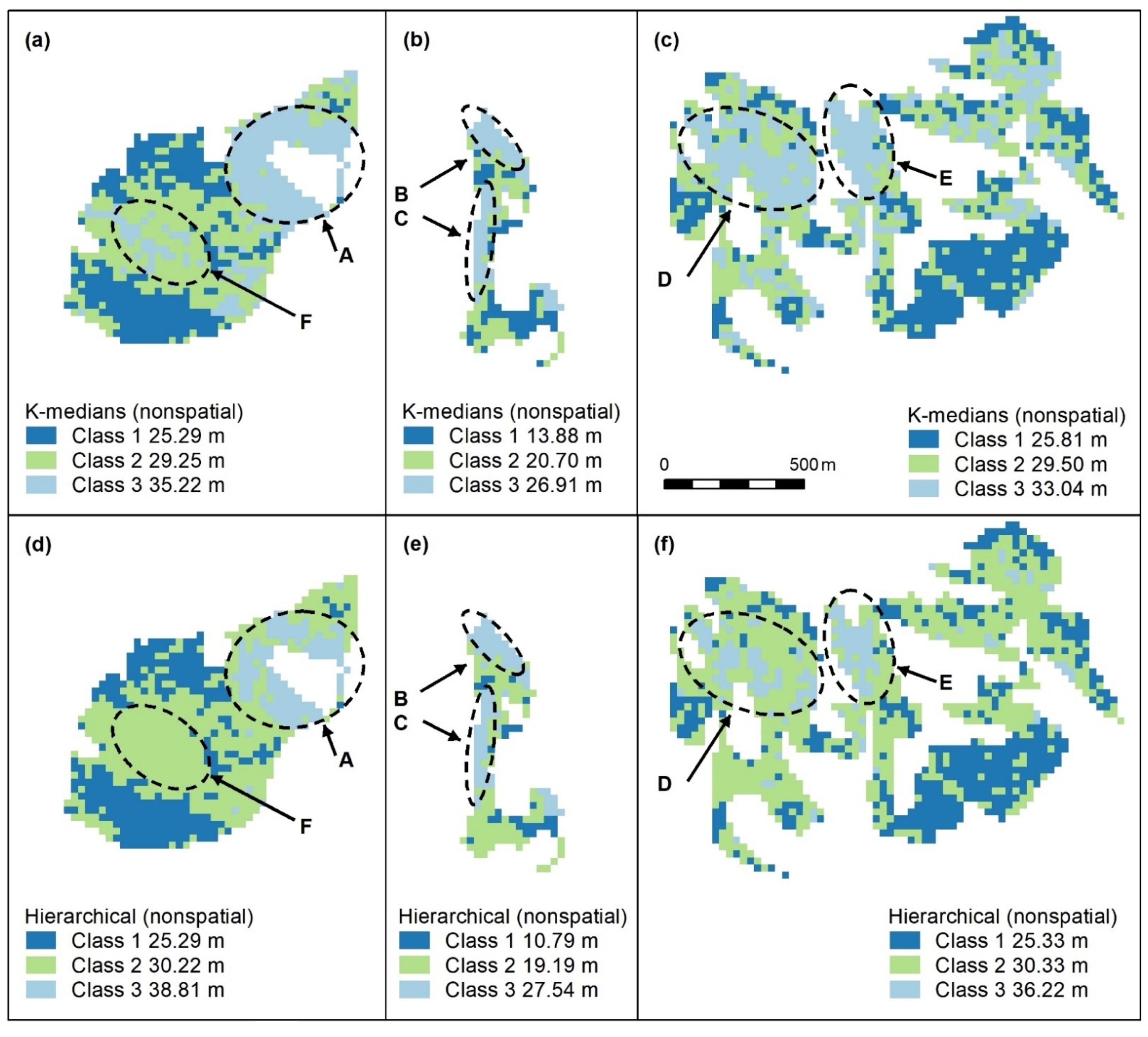
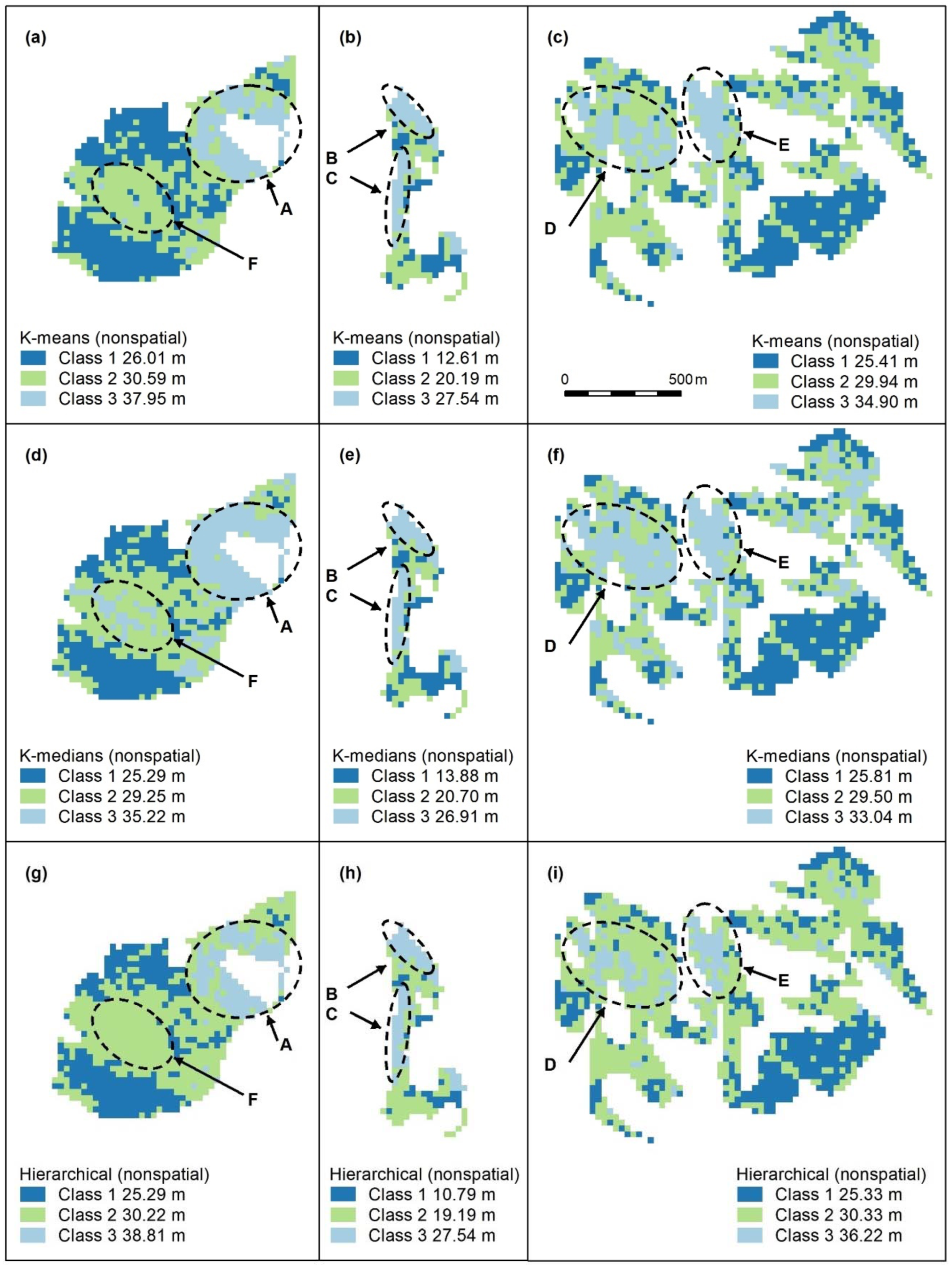
Nonspatial algorithm maps (K-means, a–c; K-medians, d–f; nonspatial hierarchical, g–i) with 3 classes. Letters A–F indicate areas of higher canopy. K-medians (d–f) best captures features A, D, C, all algorithms capture B and C. No algorithm adequately captures F, the unmapped area of Eucalyptus tereticornis. Panel scores: K-means = 12, K-medians = 16, and Hierarchical = 11.
Figure A5.
Nonspatial algorithm maps (K-means, a–c; K-medians, d–f; nonspatial hierarchical, g–i) with 3 classes. Letters A–F indicate areas of higher canopy. K-medians (d–f) best captures features A, D, C, all algorithms capture B and C. No algorithm adequately captures F, the unmapped area of Eucalyptus tereticornis. Panel scores: K-means = 12, K-medians = 16, and Hierarchical = 11.
Figure A6.
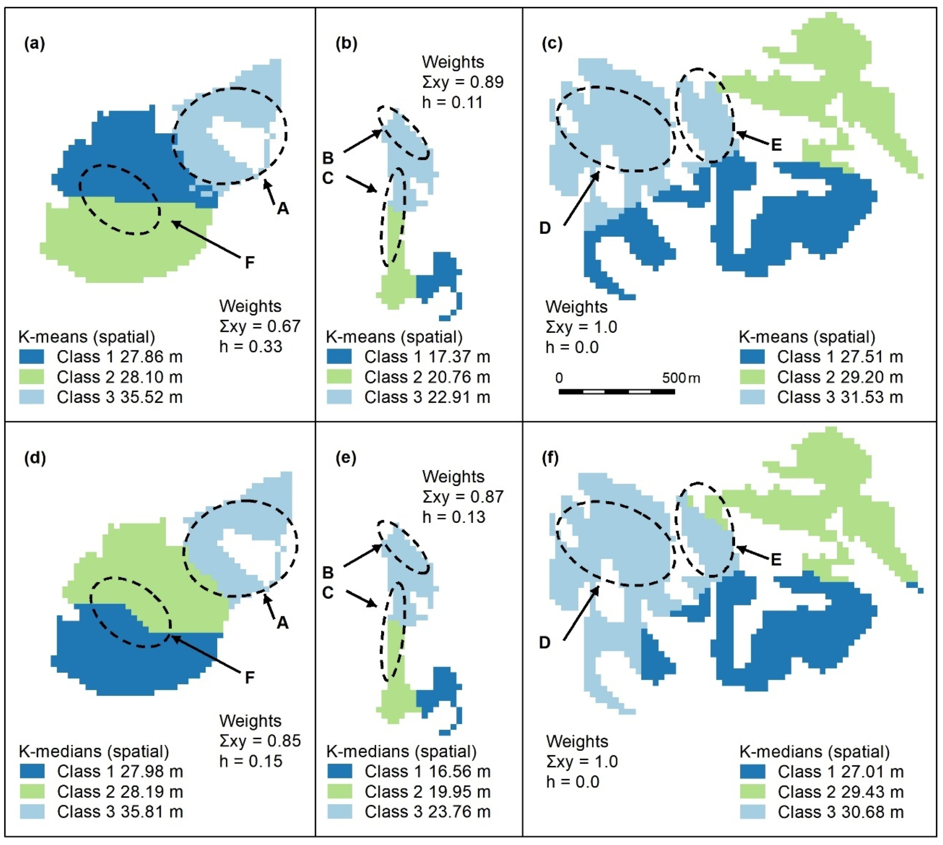
Spatially constrained K-means (a–c) and K-medians (d–f) cluster maps with 3 classes. Letters A–F indicate areas of higher canopy. Again, these algorithms use spatial weights (x, y) which outweigh those of the object (h = height). The only features adequately captured by these algorithms are A (a,d) and E (c,f). Panel scores: K-means = 9 and K-medians = 9.
Figure A6.
Spatially constrained K-means (a–c) and K-medians (d–f) cluster maps with 3 classes. Letters A–F indicate areas of higher canopy. Again, these algorithms use spatial weights (x, y) which outweigh those of the object (h = height). The only features adequately captured by these algorithms are A (a,d) and E (c,f). Panel scores: K-means = 9 and K-medians = 9.
Figure A7.
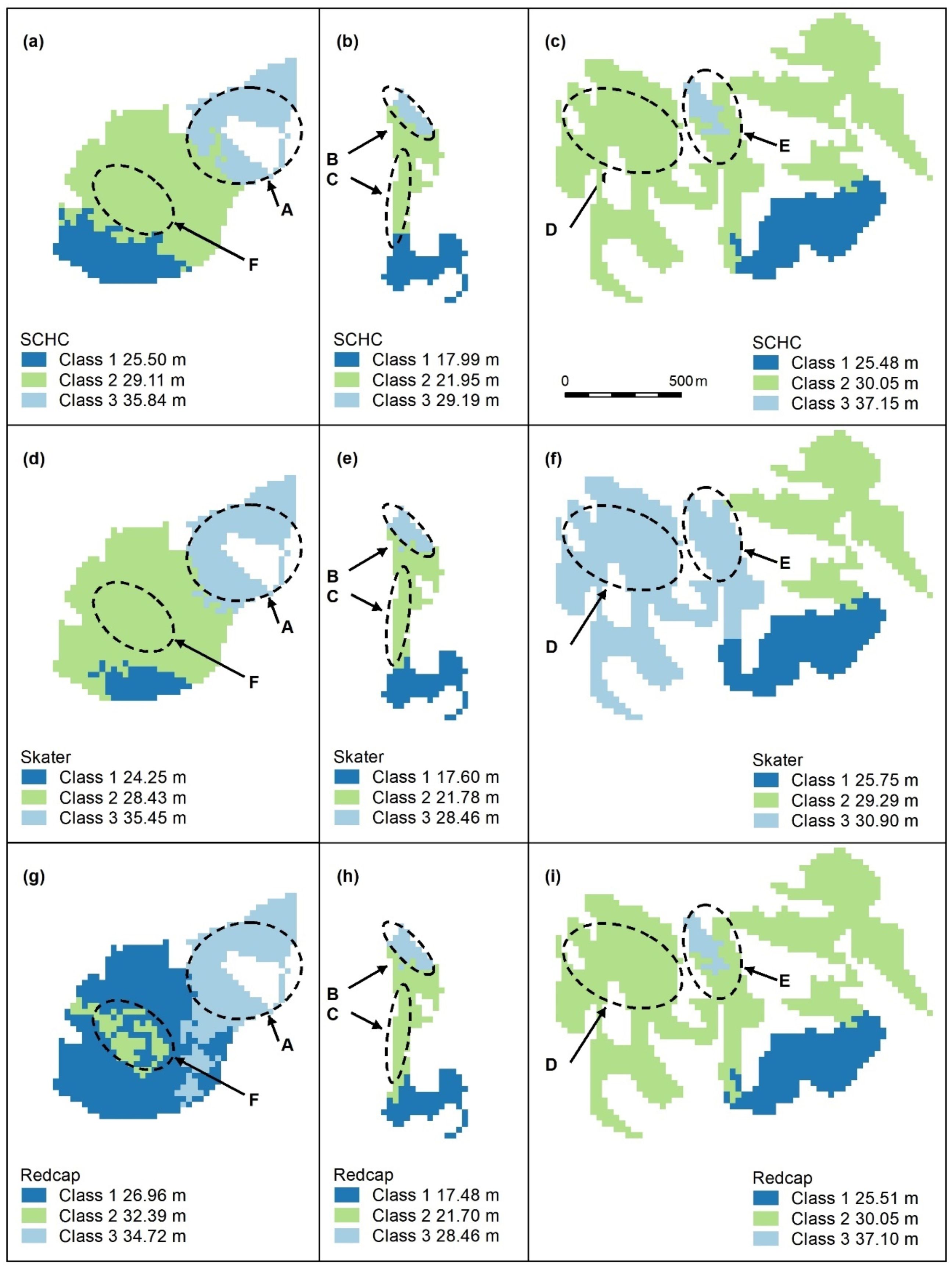
Spatially constrained hierarchical (SCHC, (a–c), Skater (d–f), and Redcap (g–i)) clustering maps with 3 classes. Letters A–F indicate areas of higher canopy, features A and B are adequately captured by all algorithms, but the areal extent of E is too small (c,i) or too large (f). C and D are not recognised. Redcap (g) separates an area of regrowth forest on land previously used for farming (dark blue) adjoining a relatively undisturbed national park (light blue), which encompasses Feature A and recognises F, the unmapped area of Eucalyptus tereticornis. Panel scores: Hierarchical clustering = 7, Skater = 9, and Redcap = 9.
Figure A7.
Spatially constrained hierarchical (SCHC, (a–c), Skater (d–f), and Redcap (g–i)) clustering maps with 3 classes. Letters A–F indicate areas of higher canopy, features A and B are adequately captured by all algorithms, but the areal extent of E is too small (c,i) or too large (f). C and D are not recognised. Redcap (g) separates an area of regrowth forest on land previously used for farming (dark blue) adjoining a relatively undisturbed national park (light blue), which encompasses Feature A and recognises F, the unmapped area of Eucalyptus tereticornis. Panel scores: Hierarchical clustering = 7, Skater = 9, and Redcap = 9.
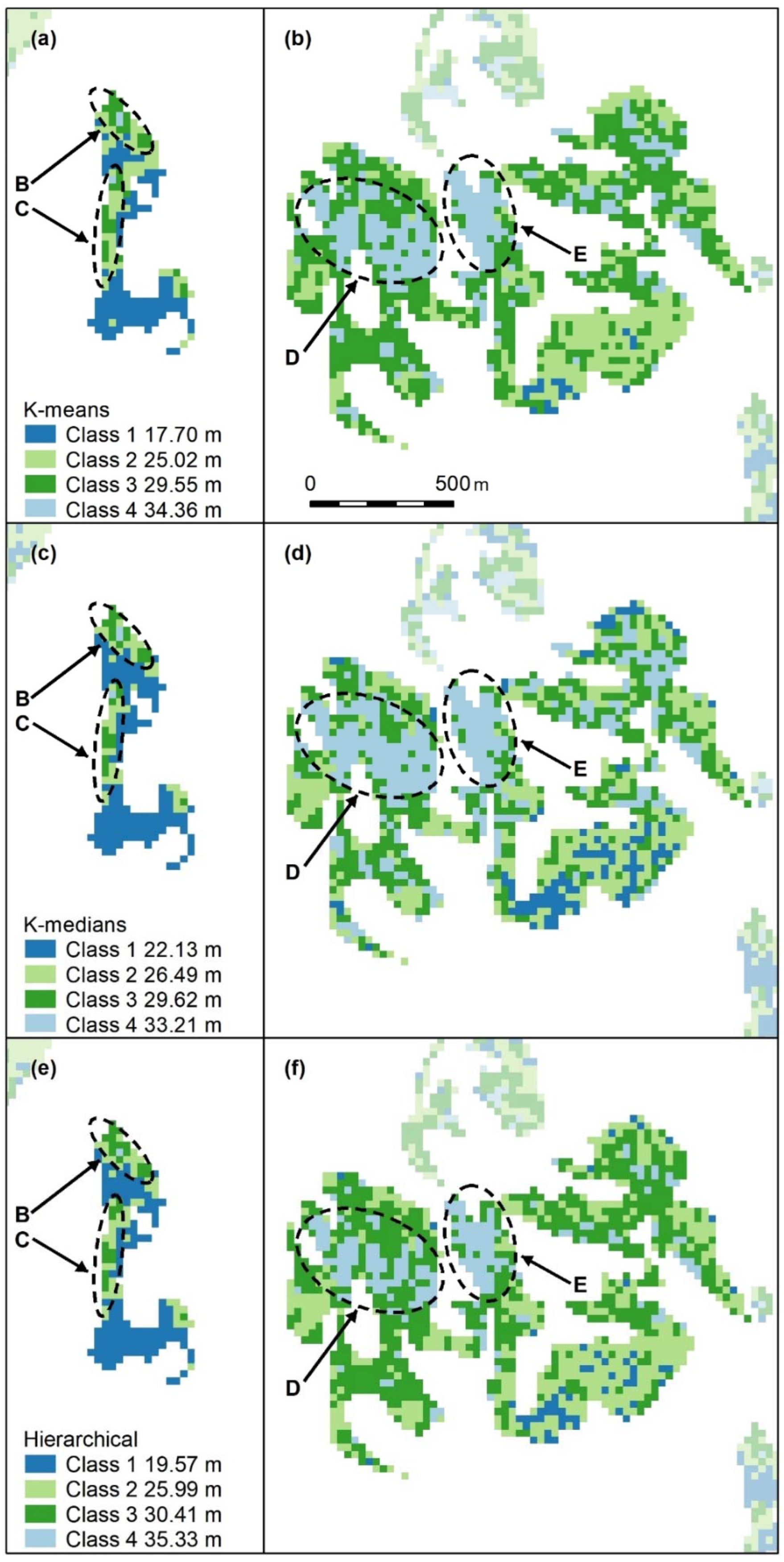
Figure A8.
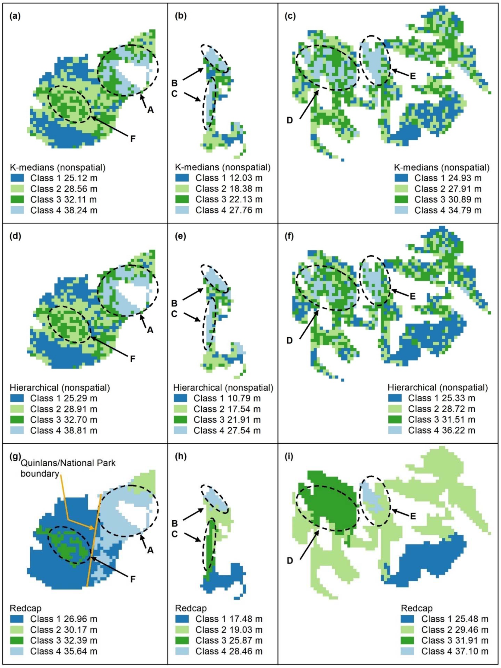
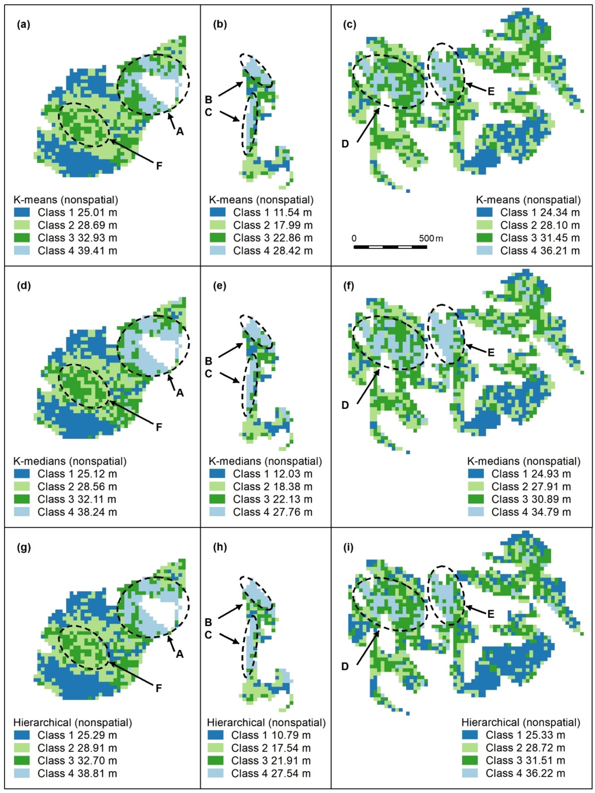
Nonspatial algorithm cluster maps, K-means (a–c), K-medians (d–f) and hierarchical (g–i) with 4 classes. Letters A–F indicate areas of higher canopy, K-medians (d–f) best captures all the features, but D and F are not contiguous. B and C are captured in all maps, with little difference between algorithms. Panel scores: K-means = 11, K-medians = 15, and Hierarchical = 12.
Figure A8.
Nonspatial algorithm cluster maps, K-means (a–c), K-medians (d–f) and hierarchical (g–i) with 4 classes. Letters A–F indicate areas of higher canopy, K-medians (d–f) best captures all the features, but D and F are not contiguous. B and C are captured in all maps, with little difference between algorithms. Panel scores: K-means = 11, K-medians = 15, and Hierarchical = 12.
Figure A9.
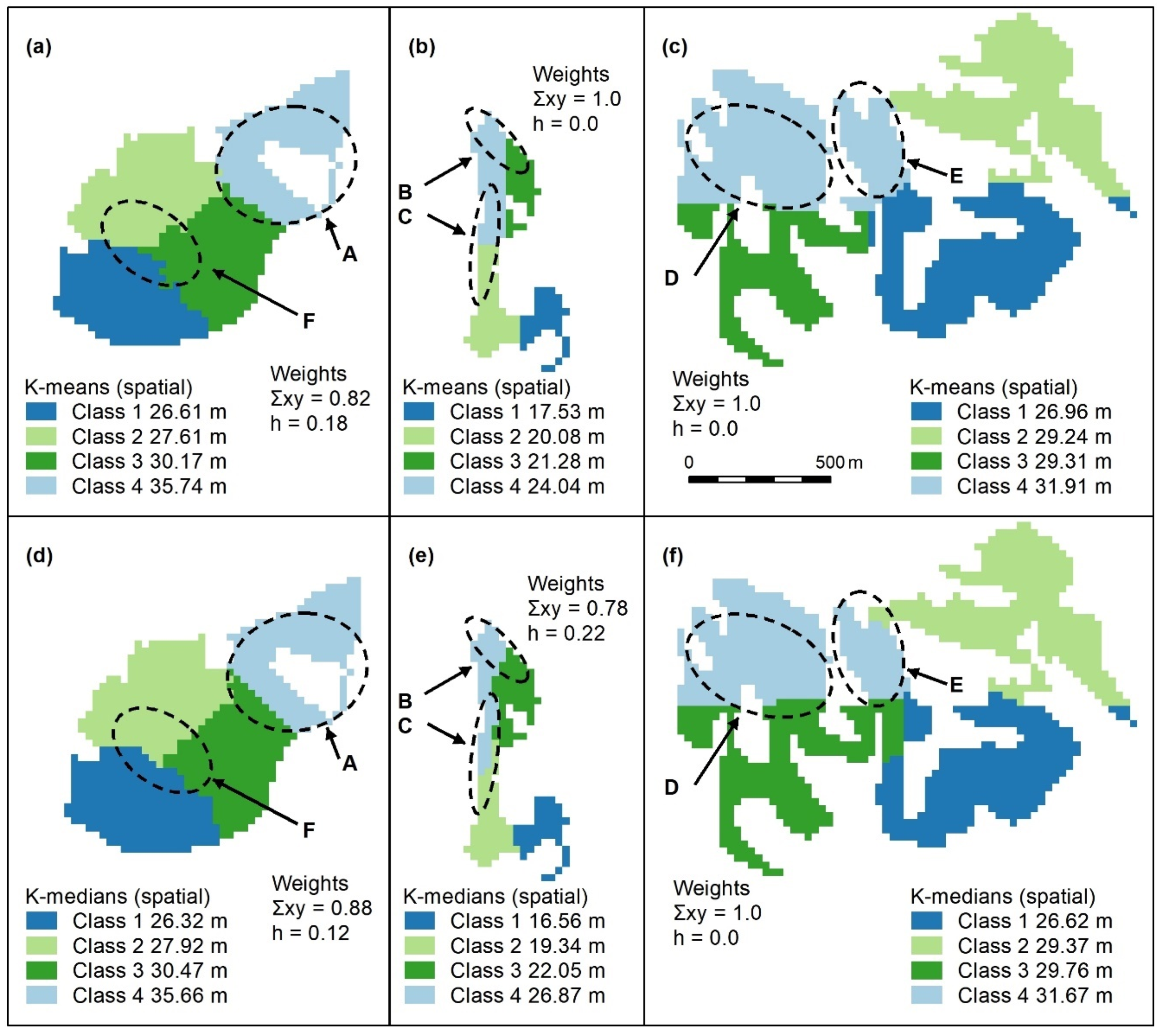
Spatially constrained K-means (a–c) and K-medians (d–f) cluster maps with 4 classes. Letters A–F indicate areas of higher canopy. Again, these algorithms use spatial weights (x, y) that far outweigh those of the object (h = height). As with 3 classes for these algorithms, the only features adequately captured are A (a,d) and E (c,f). Panel scores: K-means = 7 and K-medians = 7.
Figure A9.
Spatially constrained K-means (a–c) and K-medians (d–f) cluster maps with 4 classes. Letters A–F indicate areas of higher canopy. Again, these algorithms use spatial weights (x, y) that far outweigh those of the object (h = height). As with 3 classes for these algorithms, the only features adequately captured are A (a,d) and E (c,f). Panel scores: K-means = 7 and K-medians = 7.
Figure A10.
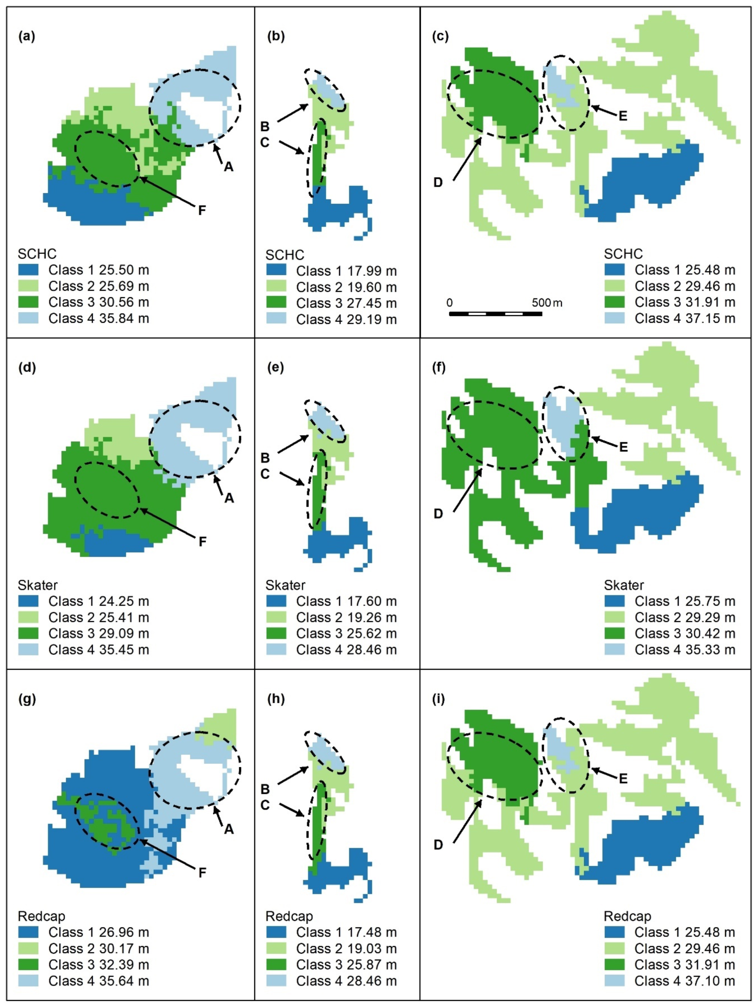
Spatially constrained hierarchical (SCHC, (a–c), Skater (d–f), and Redcap (g–i)) clustering maps with 4 classes. Letters A–F indicate areas of higher canopy. Redcap (g) separates an area of regrowth forest on land previously used for farming (A, dark blue) adjoining a relatively undisturbed national park (light blue). Redcap also recognises F, the unmapped area of Eucalyptus tereticornis (dark green), which is slightly lower in height than the national park canopy but higher than the surrounding forest (dark blue). All algorithms portray C (b,e,h) as slightly lower than B, but the areal extent of D is exaggerated by Skater (i). Skater is the algorithm that best captures the areal extent of E (i). Panel scores: Hierarchical clustering = 14, Skater = 15, and Redcap = 16.
Figure A10.
Spatially constrained hierarchical (SCHC, (a–c), Skater (d–f), and Redcap (g–i)) clustering maps with 4 classes. Letters A–F indicate areas of higher canopy. Redcap (g) separates an area of regrowth forest on land previously used for farming (A, dark blue) adjoining a relatively undisturbed national park (light blue). Redcap also recognises F, the unmapped area of Eucalyptus tereticornis (dark green), which is slightly lower in height than the national park canopy but higher than the surrounding forest (dark blue). All algorithms portray C (b,e,h) as slightly lower than B, but the areal extent of D is exaggerated by Skater (i). Skater is the algorithm that best captures the areal extent of E (i). Panel scores: Hierarchical clustering = 14, Skater = 15, and Redcap = 16.
Appendix A.3. Multiple Polygon Clustering
Non-contiguous polygons can only be clustered by nonspatial algorithms, i.e., K-means, K-medians, and hierarchical clustering. For the Koala Coast area, we selected two polygon groups, one from intra-subregional Group 6 (212 cells, 13.3 ha) and one from Group 7 (1357 cells, 84.8 ha), i.e., a polygon from each of the high- and low-canopy cohorts. We again produced a canopy height map classified by interquartile height ranges (IQR) as a reference point but with height data from 6007 cells from all seven Koala Coast intra-subregional groups (
Figure A11). Some clustering is apparent in the maps—in particular, in Map (b), two areas of higher canopy (D and E), and a section of lower canopy in the southeast. In Map (a), the higher canopy areas (B and C) are differentiated from the low-canopy height (dark blue, IQR 1).
Figure A11 thus identifies the same features as
Figure A1 but provides a subregional context, i.e., whilst B and C are higher than the remainder of their polygon group, they are significantly lower than D and E and similar areas across the subregion.
Figure A11.
Selected polygon groups from Koala Coast intra-subregional Groups 6 (
a, low-canopy cohort) and 7 (
b, high-canopy cohort). Letters B–E indicate areas of higher canopy These maps are similar to
Figure A1, with features B–E recognisable, but, because they encompass the entire canopy height range within the Koala Coast, B and C (
a) are in middle IQRs (interquartile ranges), D and E (
b) are still in the upper quartile. Lower canopy heights (
b, dark blue) adjoining B and C are pronounced. Cell colours represent the IQRs of all height data within the Koala Coast, i.e., intra-subregional Groups 1–7. IQR median heights are also shown.
Figure A12.
Nonspatial algorithm (K-means, (
a,
b), K-medians (
c,
d), hierarchical (
e,
f)) cluster maps with 2 classes. Letters B–E indicate areas of higher canopy. Features B and C (
a,
c,
e) are captured, but the areal extent of D and E (
b,
d,
f) is not as well-defined as in
Figure A11 Panel scores: K-means = 6, K-medians = 6, and Hierarchical = 7.
Figure A13.
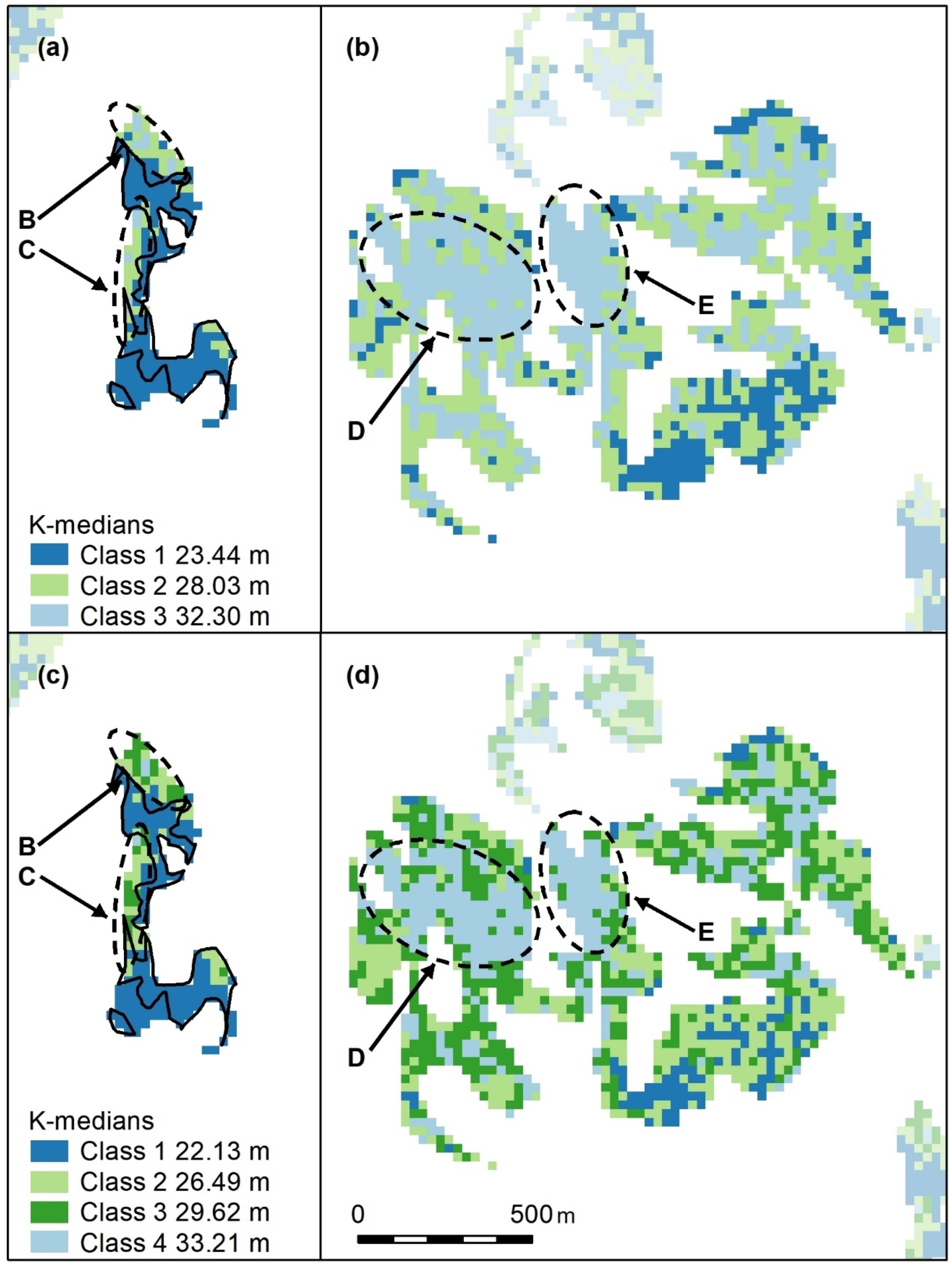
Nonspatial algorithm (K-means, a,b; K-medians c,d; hierarchical, e,f) cluster maps with 3 classes. Letters B–E indicate areas of higher canopy. Features B and C are captured by all algorithms, but D is best captured by K-means (b). Panel scores: K-means = 10, K-medians = 10, and Hierarchical = 8.
Figure A13.
Nonspatial algorithm (K-means, a,b; K-medians c,d; hierarchical, e,f) cluster maps with 3 classes. Letters B–E indicate areas of higher canopy. Features B and C are captured by all algorithms, but D is best captured by K-means (b). Panel scores: K-means = 10, K-medians = 10, and Hierarchical = 8.
Figure A14.
Nonspatial algorithm (K-means, a,b; K-medians c,d; hierarchical, e,f) cluster maps with 4 classes. Letters B–E indicate areas of higher canopy. Features B and C are captured by all algorithms, but D and E are best captured by K-medians (c,d). Panel scores: K-means = 6, K-medians = 10, and Hierarchical = 8.
Appendix A.4. Elbow Plots
Our assumption was that two, three, or four cluster class maps would have the greatest utility in terms of user practicality, but we generated maps with 2–10 clusters to allow use of the elbow method (
Figure A15,
Figure A16 and
Figure A17) to estimate the optimal number of clusters [
64]. The plots indicate that the elbow position is not clearly demarcated but occurs between two and four clusters; after four clusters, additional clusters explain less and less variance. Nonspatial methods show the greatest consistency between algorithms, and differences between spatial algorithms may be due to different polygon group shapes, i.e., compact, linear, and complex.
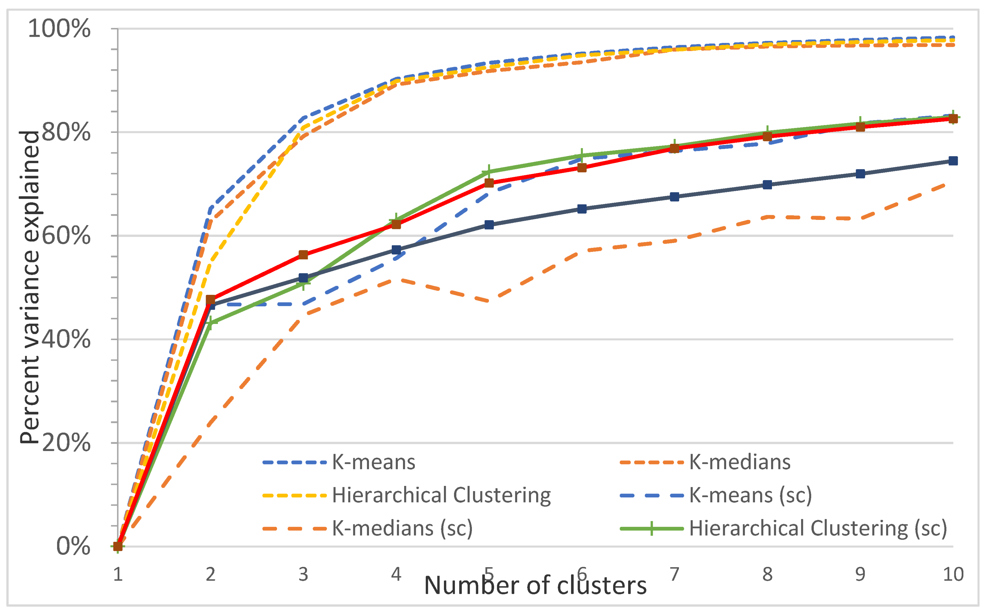
Figure A15.
Plot of the percentage of variance explained as a function of the number of clusters generated by eight algorithms for the Sunshine Coast study site. This elbow plot indicates that 2–4 classes is the optimum, e.g., for nonspatial algorithms, 3 classes explain 82.7% (K-means), 79.2% (K-medians), and 80.9% (Hierarchical clustering) of the variance, and 4 classes explain 90.3% (K-means), 89.2% (K-medians), and 90.0% (Hierarchical clustering) of the variance. In comparison, spatially constrained algorithms (sc) explain a maximum of 56% (3 classes) and 63% (4 classes) of the variance.
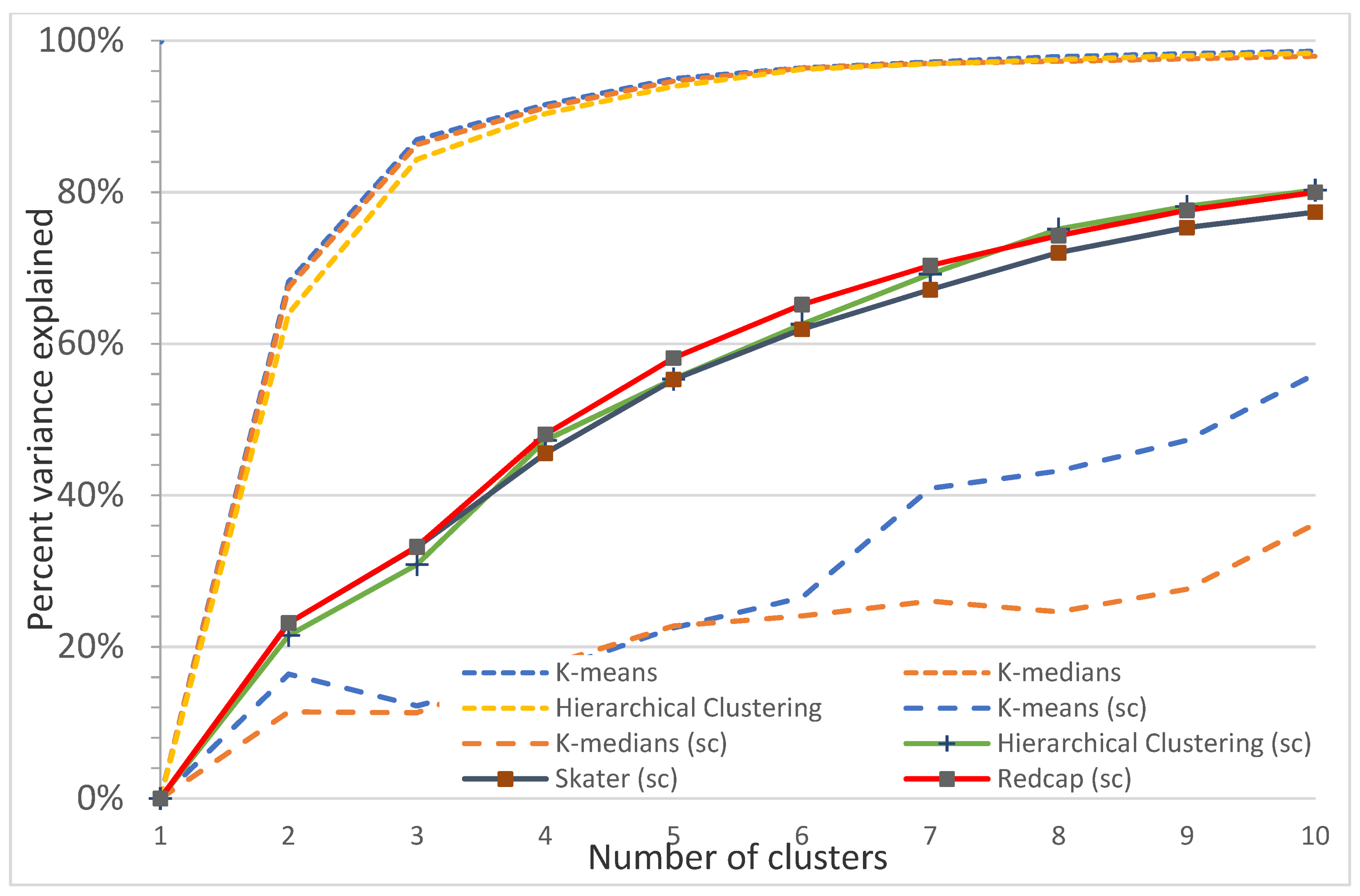
Figure A16.
Plot of percentage of the variance explained as a function of the number of clusters generated by eight algorithms for the Koala Coast intra-subregional Group 6 polygon group. This elbow plot indicates that 2 to 3 classes is the optimum, e.g., for nonspatial algorithms, 2 classes explain 86.9% (K-means), 86.3% (K-medians), and 84.3% (Hierarchical clustering) of the variance. For spatial algorithms (sc), there is no clear elbow, with the Redcap algorithm explaining a maximum of 33.2% of the variances for 3 classes.
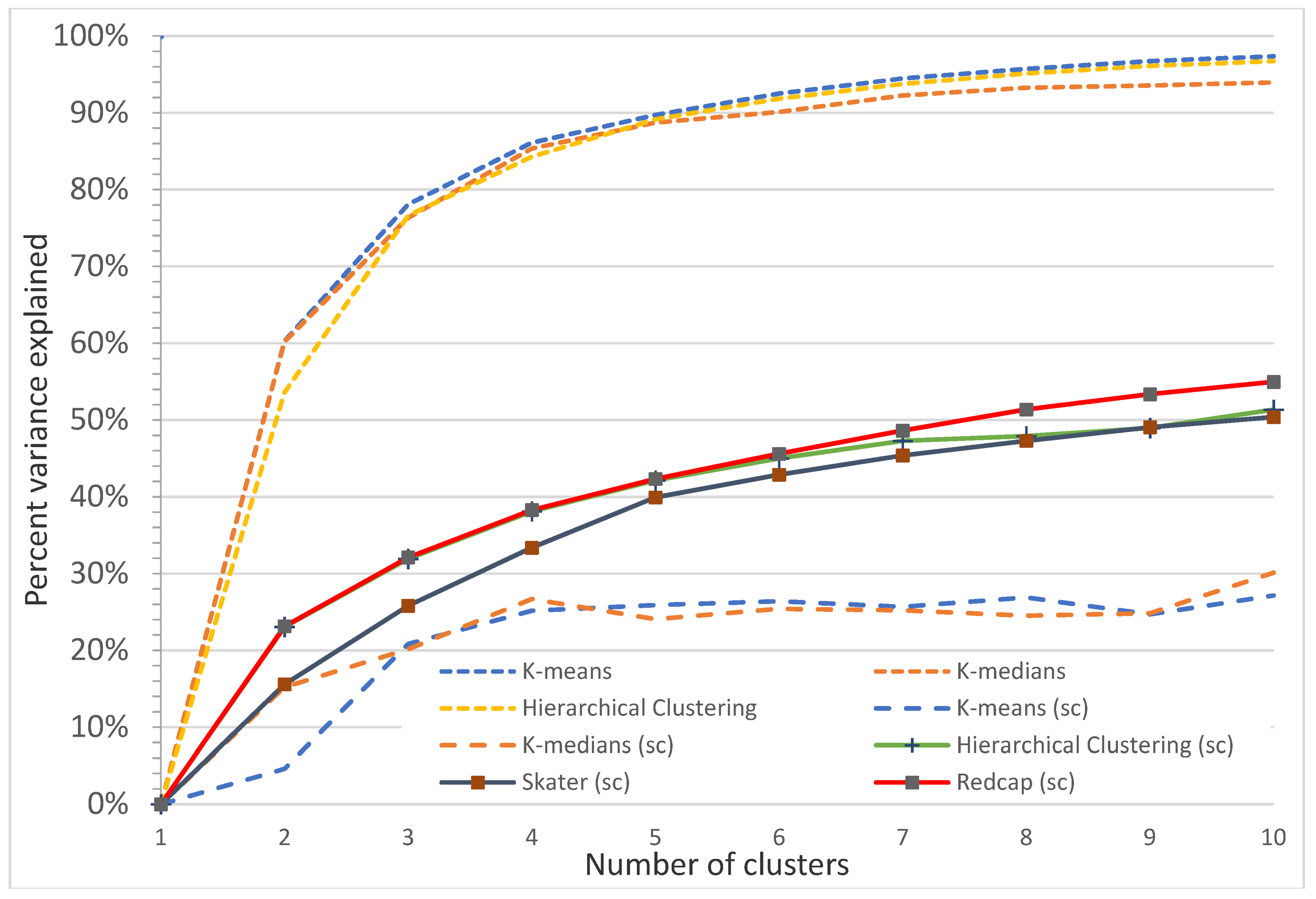
Figure A17.
Plot of percentage of the variance explained as a function of the number of clusters generated by eight algorithms for the Koala Coast intra-subregional Group 7 polygon group. This elbow plot indicates that 2–4 classes is the optimum, e.g., for nonspatial algorithms, 3 classes explain 78.1% (K-means), 76.3% (K-medians), and 76.6% (Hierarchical clustering) of the variance, and 4 classes explain 86.1% (K-means), 85.4% (K-medians), and 84.3% (Hierarchical clustering) of the variance. For spatial algorithms (sc), Redcap explains a maximum of 32.1% (3 classes) and 38.3% (4 classes) of the variance.


