
The Use of Remote Sensing Data to Estimate Land Area with Forest Vegetation Cover in the Context of Selected Forest Definitions


Abstract
:1. Background
2. Methodology
2.1. Study Site
2.2. Remotely Sensed Data
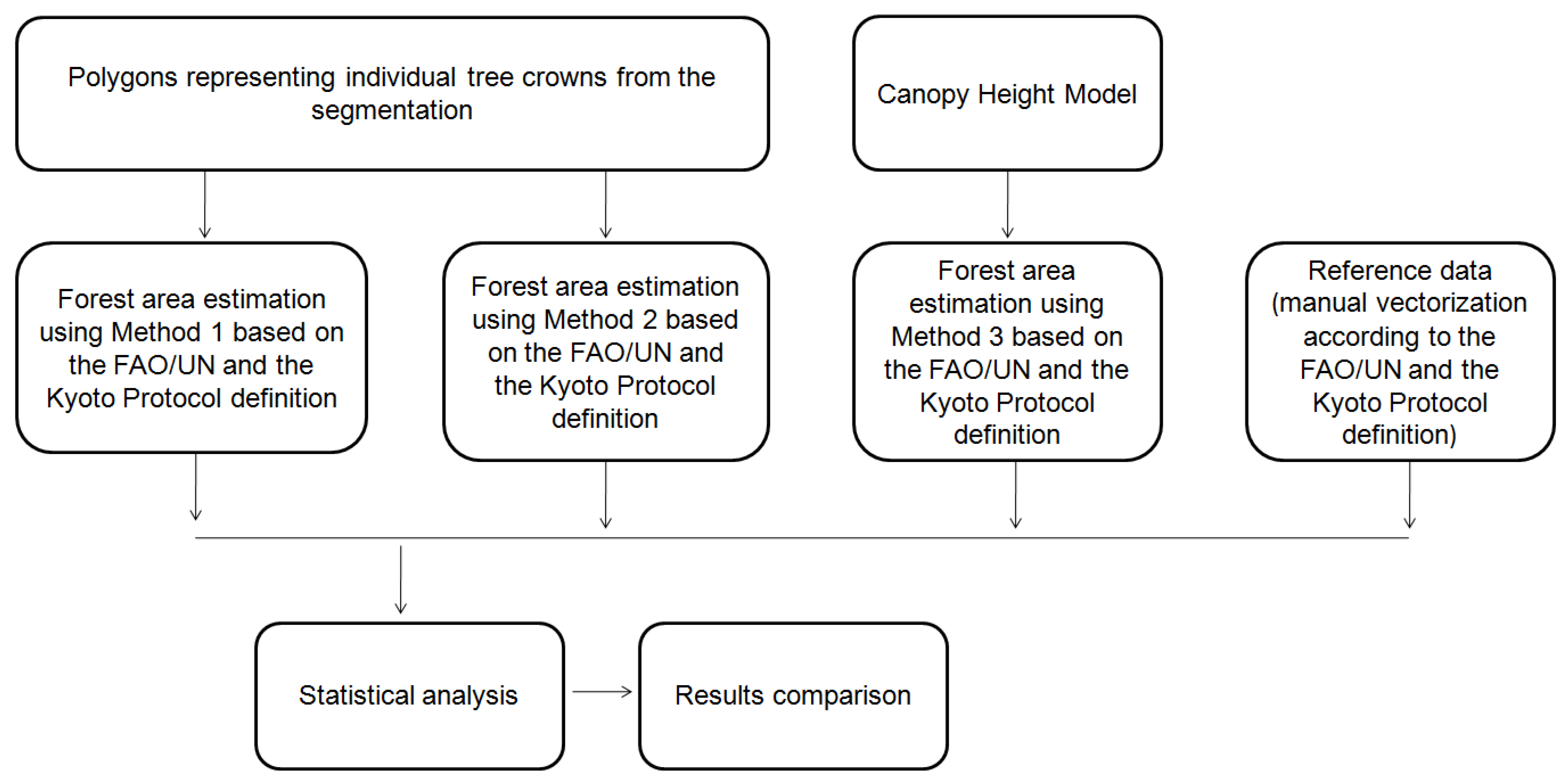
2.3. Methodology in General
2.4. Methods for Determining the Canopy Coverfrom ALS Data
2.5. The Reference Data
2.6. Statistical Analysis
2.7. Limitations of the Study
2.8. Assumptions and Boundary Conditions
3. Results
4. Discussion
5. Conclusions
Author Contributions
Funding
Institutional Review Board Statement
Informed Consent Statement
Data Availability Statement
Conflicts of Interest
Appendix A


References
- Putz, F.E.; Redford, K. The Importance of Defining ‘Forest’: Tropical Forest Degradation, Deforestation, Long-Term Phase Shifts, and Further Transitions. Biotropica 2009, 42, 10–20. [Google Scholar] [CrossRef]
- Traub, B.; Kohl, M.; Paivinen, R.; Kugler, O. Effects of different definitions on forest area estimation in national forest inventories in Europe. In Integrated Tools for Natural Resources Inventories in the 21st Century; General Technical Report NC-212; Hansen, M., Burk, T., Eds.; General Technical Report NC-212; U.S. Dept. of Agriculture, Forest Service, North Central Forest Experiment Station: St. Paul, MN, USA, 2000; pp. 176–184. [Google Scholar]
- Mathys, L.; Ginzler, C.; Zimmermann, E.; Brassel, P.; Wildi, O. Sensitivity assessment on continuous landscape variables to classify a discrete forest area. For. Ecol. Manag. 2006, 229, 111–119. [Google Scholar] [CrossRef]
- Colson, F.; Bogaert, J.; Filho, A.C.; Nelson, B.; Pinage, E.R. The influence of forest definition on landscape fragmentation assessment in Rondônia, Brazil. Ecol. Indic. 2009, 9, 1163–1168. [Google Scholar] [CrossRef]
- Seebach, L.M.; Strobl, P.; San Miguel-Ayanz, J.; Gallego, J.; Bastrup-Birk, A. Comparative analysis of harmonized forest area estimates for European countries. Int. J. For. Res. 2011, 84, 285–299. [Google Scholar] [CrossRef] [Green Version]
- Romijn, E.; Ainembabazi, J.H.; Wijaya, A.; Herold, M.; Angelsen, A.; Verchot, L.; Murdiyarso, D. Exploring different forest definitions and their impact on developing REDD+ reference emission levels: A case study for Indonesia. Environ. Sci. Policy 2013, 33, 246–259. [Google Scholar] [CrossRef]
- Sasaki, N.; Putz, F.E. Crucial need for new definitions of “forest” and “forest degradation” in global climate change agreements. A J. Soc. Conserv. Biol. 2009, 2, 226–232. [Google Scholar]
- Mayeux, P.; Frederic, A.; Malingeau, J.P. Global tropical forest area measurements derived from coarse resolution satellite imagery: A comparison with other approaches. Environ. Conserv. 1998, 25, 37–52. [Google Scholar] [CrossRef]
- FAO. Global Forest Resources Assessment Update 2005, Terms and Definitions. In Forest Resources Assessment (2004) Working Paper 83; FAO: Rome, Italy, 2005. [Google Scholar]
- FAO. Specification of National Reporting Tables for FRA 2010. In Forest Resources Assessment (2007) Working Paper 135; FAO: Rome, Italy, 2010. [Google Scholar]
- FAO. Forest Resources Assessment Update 2015, Terms and Definitions. In Forest Resources Assessment (2012) Working Paper 180; FAO: Rome, Italy, 2015. [Google Scholar]
- Decision 2/CMP.7. Land use, land−use change and forestry (2012). In Proceedings of the Report of the Conference of the Parties serving as the meeting of the Parties to the Kyoto Protocol on Its Seventh Session, Durban, South African, 28 November–11 December 2011. [Google Scholar]
- Jabłoński, M. Definicja lasu w ujęciu krajowym i międzynarodowym oraz jej znaczenie dla wielkości i zmian powierzchni lasów w Polsce. Sylwan 2015, 159, 469–482. [Google Scholar]
- Jabłoński, M. Powierzchnia lasów. Definicja definicji nierówna. Las Pol. 2015, 24, 24–26. [Google Scholar]
- Jabłoński, M. Powierzchnia gruntów leśnych—Przyczyny zmian i spójność źródeł danych. Wiadomości Stat. 2015, 11, 54–68. [Google Scholar]
- Jabłoński, M.; Korhonen, K.T.; Budniak, P.; Mionskowski, M.; Zajączkowski, G.; Sućko, K. Comparing land use registry and sample based inventory to estimate forest area in Podlaskie, Poland. iForest 2017, 10, 315–321. [Google Scholar] [CrossRef] [Green Version]
- Neef, T.; von Luepke, H.; Schoene, D. Choosing a Forest Definition for the Clean Development Mechanism; FAO: Rome, Italy, 2006; pp. 1–18. [Google Scholar]
- Próchnicki, P. Wykorzystanie GIS i teledetekcji jako narzędzi do analizy sukcesji zakrzewień w Narwiańskim Parku Narodowym. Rocz. Geomatyki 2006, 4, 127–134. [Google Scholar]
- Kunz, M.; Nienartowicz, A.; Deptuła, M. Teledetekcja satelitarna wtórnych lasów na gruntach porolnych na przykładzie Zaborskiego Parku Krajobrazowego. Fotointerpret. W Geogr. 2000, 31, 122–128. [Google Scholar]
- Haapanen, R.; Ek, A.R.; Bauer, M.E.; Finley, E.O. Delineation of forest/non forest land use classes using nearest neighbor methods. Remote Sens. Environ. 2004, 89, 265–271. [Google Scholar] [CrossRef]
- McRoberts, R.E. Satellite image-based maps: Scientific inference or pretty pictures. Remote Sens. Environ. 2011, 115, 715–724. [Google Scholar] [CrossRef]
- McRoberts, R.E.; Gobakken, T.; Naesset, E. Post-stratified estimation of forest area and growing stock volume using lidar-based stratifications. Remote Sens. Environ. 2012, 125, 157–166. [Google Scholar] [CrossRef]
- Stehman, S.V.; Foody, G.M. Key issues in rigorous accuracy assessment of land cover products. Remote Sens. Environ. 2019, 231, 111199. [Google Scholar] [CrossRef]
- Stehman, S.V. Estimating area from an accuracy assessment error matrix. Remote Sens. Environ. 2013, 132, 202–211. [Google Scholar] [CrossRef]
- Olofsson, P.; Foody, G.M.; Herold, M.; Stehman, S.V.; Woodcock, C.E.; Wulder, M.A. Good practices for estimating area and assessing accuracy of land change. Remote Sens. Environ. 2014, 148, 42–57. [Google Scholar] [CrossRef]
- Naesset, E.; Orka, H.O.; Solberg, S.; Bollandsas, O.M.; Hansen, E.H.; Mauya, E.; Zahabu, E.; Malimbwi, R.; Chamuya, N.; Olsson, H.; et al. Mapping and estimating forest area and aboveground biomass in miombo woodlands in Tanzania using data from airborne. Remote Sens. Environ. 2016, 175, 282–300. [Google Scholar] [CrossRef]
- Wang, Z.; Boesch, R.; Ginzler, C. Integration of high resolution aerial images and airborne Lidar data for forest delineation. In Proceedings of the International Archives of the Photogrammetry, Remote Sensing and Spatial Information Sciences 37 (B7), Beijing, China, 3–11 July 2008. [Google Scholar]
- Wang, Z.; Boesch, R.; Ginzler, C. Color and LiDAR data fusion: Application to automatic forest boundary delineation in aerial images. Int. Arch. Photogramm. Remote Sens. Spat. Inf. Sci. 2007, 3, 1203–1207. [Google Scholar]
- Wang, Z.; Boesch, R.; Ginzler, C. Aerial images and LIDAR Fusion Applied in Forest Boundary. In Proceedings of the 7th WSEAS International Conference on Signal, Speech and Image Processing, Beijing, China, 15–17 September 2007. [Google Scholar]
- Pekkarinen, A.; Reithmaier, L.; Strobl, P. Pan-European forest/non-forest mapping with Landsat ETM+ and CORINE Land Cover 2000 data. J. Photogramm. Remote Sens. 2009, 64, 171–183. [Google Scholar] [CrossRef]
- Hościłło, A.; Mirończuk, A.; Lewandowska, A.; Gąsiorowski, J. Inventory of the Actual Forest Cover of the Country Using the Existing Photogrammetric Data; Institute of Geodesy and Cartography: Warsaw, Poland, 2015. [Google Scholar]
- Thompson, S.D.; Nelson, T.A.; Giesbrecht, I.; Frazer, G.; Saunders, S.C. Data-driven regionalization of forested and non-forested ecosystems in coastal British Columbia with LiDAR and RapidEye imagery. Appl. Geogr. 2016, 69, 35–50. [Google Scholar] [CrossRef]
- Wężyk, P.; de Kok, R. Automatic Mapping of the Dynamics of Forest Successionon Abandoned Parcels in South Poland. Angew. Geoinformatik 2005, 1–6. [Google Scholar]
- Kolecka, N.; Kozak, J.; Kaim, D.; Dobosz, M.; Ginzler, C.; Psomas, A. Mapping Secondary Forest Succession on Abandoned Agricultural Land with LiDAR Point Clouds and Terrestrial Photography. Remote Sens. 2015, 7, 8300–8322. [Google Scholar] [CrossRef] [Green Version]
- Szostak, M.; Hawryło, P.; Piela, P. Using of Sentinel-2 images for automation of the forest succession detection. Eur. J. Remote Sens. 2018, 51, 142–149. [Google Scholar] [CrossRef]
- Pujar, G.S.; Reddy, P.M.; Reddy, C.S.; Jha, C.S.; Dadhwal, V.K. Estimation of Trees Outside Forests using IRS High Resolution data by Object Based Image Analysis. In Proceedings of the International Archives of the Photogrammetry, Remote Sensing and Spatial Information Sciences XL-8, Hyderabad, India, 9–12 December 2014; pp. 623–629. [Google Scholar]
- Castillo-Núñez, M.; Sánchez-Azofeifa, A.; Croitoru, A.; Rivard, B.; Calvo-Alvarado, J.; Dubayah, R.O. Delineation of secondary succession mechanisms for tropical dry forests using LiDAR. Remote Sens. Environ. 2011, 115, 2217–2231. [Google Scholar] [CrossRef]
- Vega, C.; Durrieu, S. Multi-level filtering segmentation to measure individual tree parameters based on Lidar data: Application to a mountainous forest with heterogeneous stands. Int. J. Appl. Earth Obs. Geoinf. 2011, 13, 646–656. [Google Scholar] [CrossRef] [Green Version]
- Vega, C.; Hamrouni, A.; El Mokhtari, S.; Morel, J.; Bock, J.; Renaud, J.-P.; Bouvier, M.; Durrieu, S. PTrees: A point-based approach to forest tree extraction from lidar data. Int. J. Appl. Earth Obs. Geoinf. 2014, 33, 98–108. [Google Scholar] [CrossRef]
- Swetnam, T.L.; Falk, D.A. Application of Metabolic Scaling Theory to reduce error in local maxima tree segmentation from aerial LiDAR. For. Ecol. Manag. 2014, 323, 158–167. [Google Scholar] [CrossRef]
- Strimbu, V.F.; Strimbu, B.M. A graph-based segmentation algorithm for tree crown extraction using airborne LiDAR data. ISPRS J. Photogramm. Remote Sens. 2015, 104, 30–43. [Google Scholar] [CrossRef] [Green Version]
- Latifi, H.; Fassnacht, F.E.; Muller, J.; Tharani, A.; Dech, S.; Heurich, M. Forest inventories by LiDAR data: A comparison of single tree segmentation and metric-based methods for inventories of a heterogeneous temperate forest. Int. J. Appl. Earth Obs. Geoinf. 2015, 42, 162–174. [Google Scholar] [CrossRef]
- Mongus, D.; Zalik, B. An efficient approach to 3D single tree-crown delineation in LiDAR data. ISPRS J. Photogramm. Remote Sens. 2015, 108, 219–233. [Google Scholar] [CrossRef]
- Ferraz, A.; Saatchi, S.; Mallet, C.; Meyer, V. Lidar detection of individual tree size in tropical forests. Remote Sens. Environ. 2016, 183, 318–333. [Google Scholar] [CrossRef]
- Hamraz, H.; Contrares, M.A.; Zhang, J. A scalable approach for tree segmentation within small-footprint airborne LiDAR data. Comput. Geosci. 2017, 102, 139–147. [Google Scholar] [CrossRef] [Green Version]
- Hamraz, H.; Contrares, M.A.; Zhang, J. A robust approach for tree segmentation in deciduous forests using small-footprint airborne LiDAR data. Int. J. Appl. Earth Obs. Geoinf. 2016, 52, 532–541. [Google Scholar] [CrossRef] [Green Version]
- Wu, B.; Yu, B.; Wu, Q.; Huang, Y.; Chen, Z.; Wu, J. Individual tree crown delineation using localized contour tree method and airborne LiDAR data in coniferous forests. Int. J. Appl. Earth Obs. Geoinf. 2016, 52, 82–94. [Google Scholar] [CrossRef]
- Kamińska, A.; Lisiewicz, M.; Stereńczak, K.; Kraszewski, B.; Sadkowski, R. Species-related single dead tree detection using multi-temporal ALS data and CIR imagery. Remote Sens. Environ. 2018, 219, 31–43. [Google Scholar] [CrossRef]
- Magdon, P.; Kleinn, C. Uncertainties of forest area estimates caused by the minimum crown cover criterion-a scale issue relevant to forest cover monitoring. Environ. Monit. Assess. 2013, 185, 5345–5360. [Google Scholar] [CrossRef] [PubMed] [Green Version]
- Eysn, L.; Hollaus, M.; Schadauer, K.; Pfeifer, N. Forest Delineation Based on Airborne LIDAR Data. Remote Sens. 2012, 4, 762–783. [Google Scholar] [CrossRef] [Green Version]
- Eysn, L.; Hollaus, M.; Schadauer, K.; Pfeifer, N.; Roncat, A. Crown coverage calculation based on ALS data. In Proceedings of the 11th International Conference on LiDAR Applications for Assessing Forest Ecosystems—SilviLaser 2011, Hobart, Australia, 16–20 October 2011. [Google Scholar]
- Eysn, L.; Hollaus, M.; Vetter, M.; Mücke, W.; Pfeifer, N.; Regner, B. Adapting alpha-shapes for forest delineation using ALS Data. In Proceedings of the 10th International Conference on LiDAR Applications for Assessing Forest Ecosystems—Silvilaser 2010, Freiburg, Germany, 14–17 September 2010. [Google Scholar]
- Sackov, I.; Kardos, M. Forest delineation based on LiDAR data and vertical accuracy of the terrain model in forest and non-forest area. Ann. For. Res. 2014, 57, 119–136. [Google Scholar] [CrossRef]
- Straub, C.; Weinacker, H.; Koch, B. A fully automated procedure for delineation and classification of forest and non-forest vegetation based on full waveform laser scanner data. In Proceedings of the International Archives of the Photogrammetry, Remote Sensing and Spatial Information Sciences 37 (B8), Beijing, China, 3–11 July 2008. [Google Scholar]
- Szwagrzyk, J. Sukcesja leśna na gruntach porolnych; stan obecny, prognozy i wątpliwości. Sylwan 2017, 4, 53–59. [Google Scholar]
- Milicz Forest District Website. Available online: https://milicz.wroclaw.lasy.gov.pl (accessed on 16 March 2020).
- Stereńczak, K.; Lisańczuk, M.; Parkitna, K.; Mitelsztedt, K.; Mroczek, P.; Miścicki, S. The influence of number and size of sample plots on modelling growning stock volume based on airborne laser scanning. Drewno 2018, 61, 5–22. [Google Scholar]
- Stereńczak, K.; Kraszewski, B.; Mielcarek, M.; Piasecka, Ż.; Lisiewicz, M.; Heurich, M. Mapping individual trees with airborne laser scanning data in an European lowland forest using a self-calibration algorithm. Int. J. Appl. Earth Obs. Geoinf. 2020, 93, 102191. [Google Scholar] [CrossRef]
- Mielcarek, M.; Kamińska, A.; Stereńczak, K. Digital Aerial Photogrammetry (DAP) and Airborne Laser Scanning (ALS) as Sources of Information about Tree Height: Comparisons of the Accuracy of Remote Sensing Methods for Tree Height Estimation. Remote Sens. 2020, 12, 1808. [Google Scholar] [CrossRef]
- Ciesielski, M.; Stereńczak, K. Volunteered Geographic Information data as a source of information on the use of forests in the Warsaw agglomeration. Sylwan 2020, 164, 695–704. [Google Scholar]
- Ciesielski, M.; Stereńczak, K. What do we expect from forests? The European view of public demands. J. Environ. Manag. 2018, 209, 139–151. [Google Scholar] [CrossRef] [PubMed]


| Land Area | Evergreen and Tropical Rain Forest | Tropical Rain Forest | Wet, Moist and Mountain Forest | Closed Broadleaved Forest | Closed Forest | |
|---|---|---|---|---|---|---|
| Central Africa | 398,320 | 183,967 | 78,821 | 202,456 | 158,300 | 185,802 |
| West Africa | 203,803 | 17,859 | 3231 | 52,223 | 15,569 | 13,470 |
| Total Africa | 602,123 | 201,826 | 82,052 | 254,679 | 173,869 | 199,273 |
| Central America | 50,977 | 18,029 | 11,957 | 21,525 | 17,499 | 22,649 |
| Caribbean-Mexico | 202,934 | 32,858 | 267 | 746,763 | 10,130 | 54,321 |
| South America | 1,002,297 | 652,772 | 438,932 | 715,509 | 637,050 | 615,605 |
| Variables | Law on Forests—Poland | FAO | Kyoto Protocol |
|---|---|---|---|
| Minimum area (ha) | 0.1 | 0.5 | 0.1 |
| Minimum height (m) | - | 5 | 2 |
| Minimum crown coverage (%) | - | 10 | 10 |
| Width of the forest complex (m) | - | - | 10 |
| Land intended for renovation | yes | yes | yes |
| Land intended for natural succession | yes | yes | yes |
| Hunting plots | yes | yes | yes/no |
| Christmas tree plantations | yes | yes | yes |
| Post-agricultural land with secondary succession | no | yes | yes |
| Land related to forest management | yes | yes | no |
| Orchards and urban greenery | no | no | yes |
| Scheme | Habitat | Species | Age | Volume |
|---|---|---|---|---|
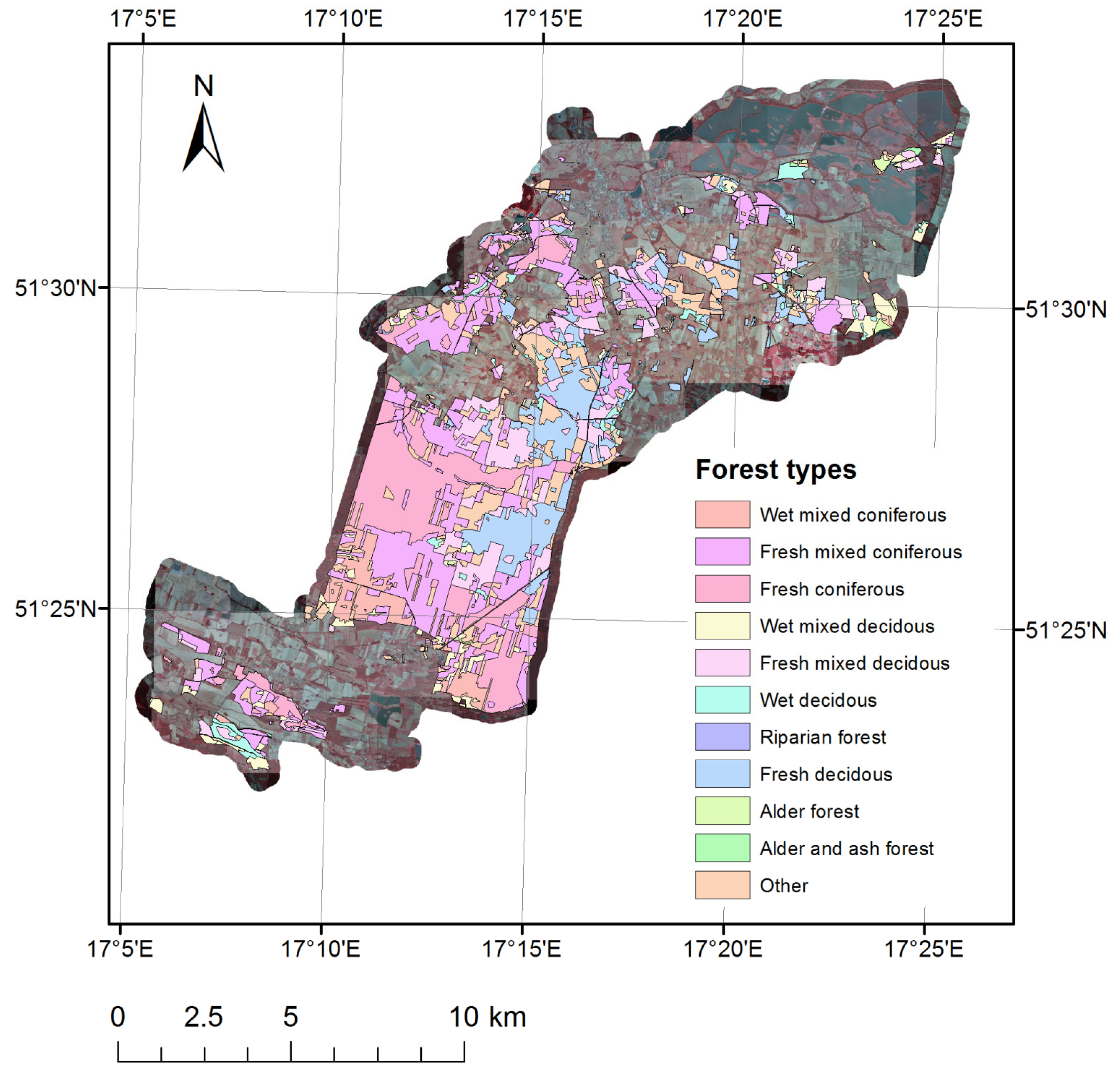
| Milicz Forest Department | Fresh coniferous—19.2% (1572.3 ha) Fresh mixed coniferous—26.8% (2198.1 ha) Wet mixed coniferous—5.1% (413.9 ha) Fresh deciduous—13.5% (1105.1 ha) Fresh mixed deciduous—13.1% (1072.2 ha) Wet mixed deciduous—4.5% (369.4 ha) Wet deciduous—2.6% (216.5 ha) | Pine—74.9% (1,973,262.2 ha) Oak—10.6% (279,260.1 ha) Beech—5.8% (152,802.7 ha) Birch—2% (52,690.6 ha) Alder—4.7% (2476.5 ha) Other—2% (52,690.6 ha) | 0–20—12% (316,143.5 ha) 20–40—15% (395,179.4 ha) 40–60—29.6% (779,820.6 ha) 60–80—13.6% (358,295.9 ha) 80–100—12.7% (334,585.2 ha) >100—15.6% (410,986.5 ha) | Beech—300 m3/ha Pine—298 m3/ha Alder—285 m3/ha Oak = 275 m3/ha |
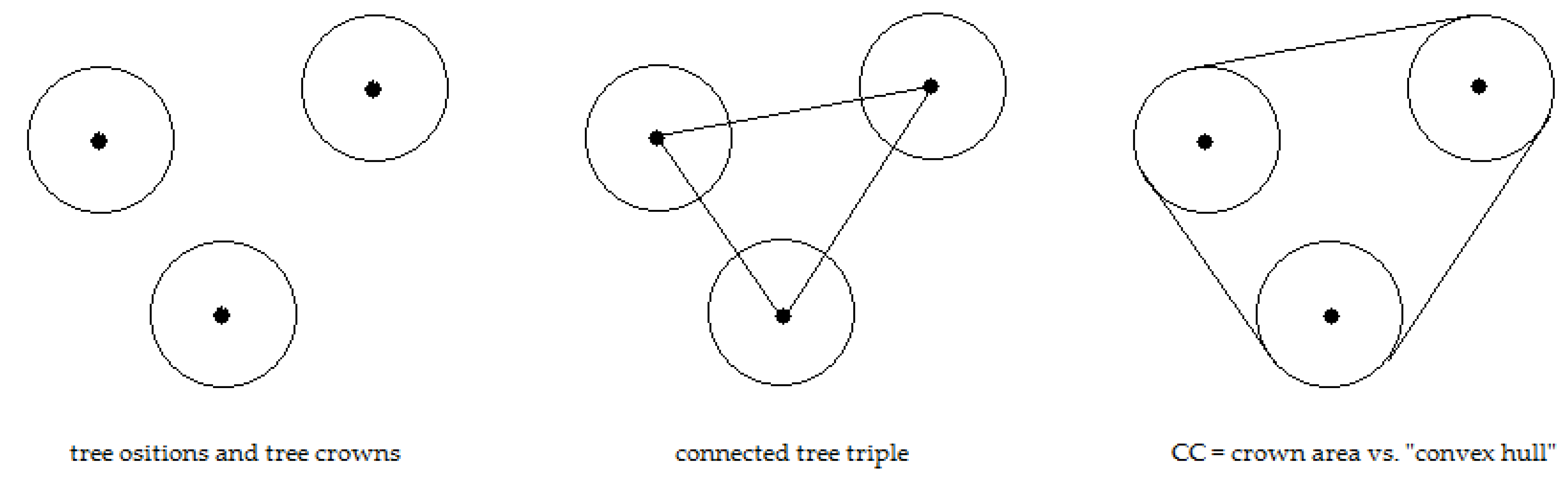
| Method | Reference | Description |
|---|---|---|
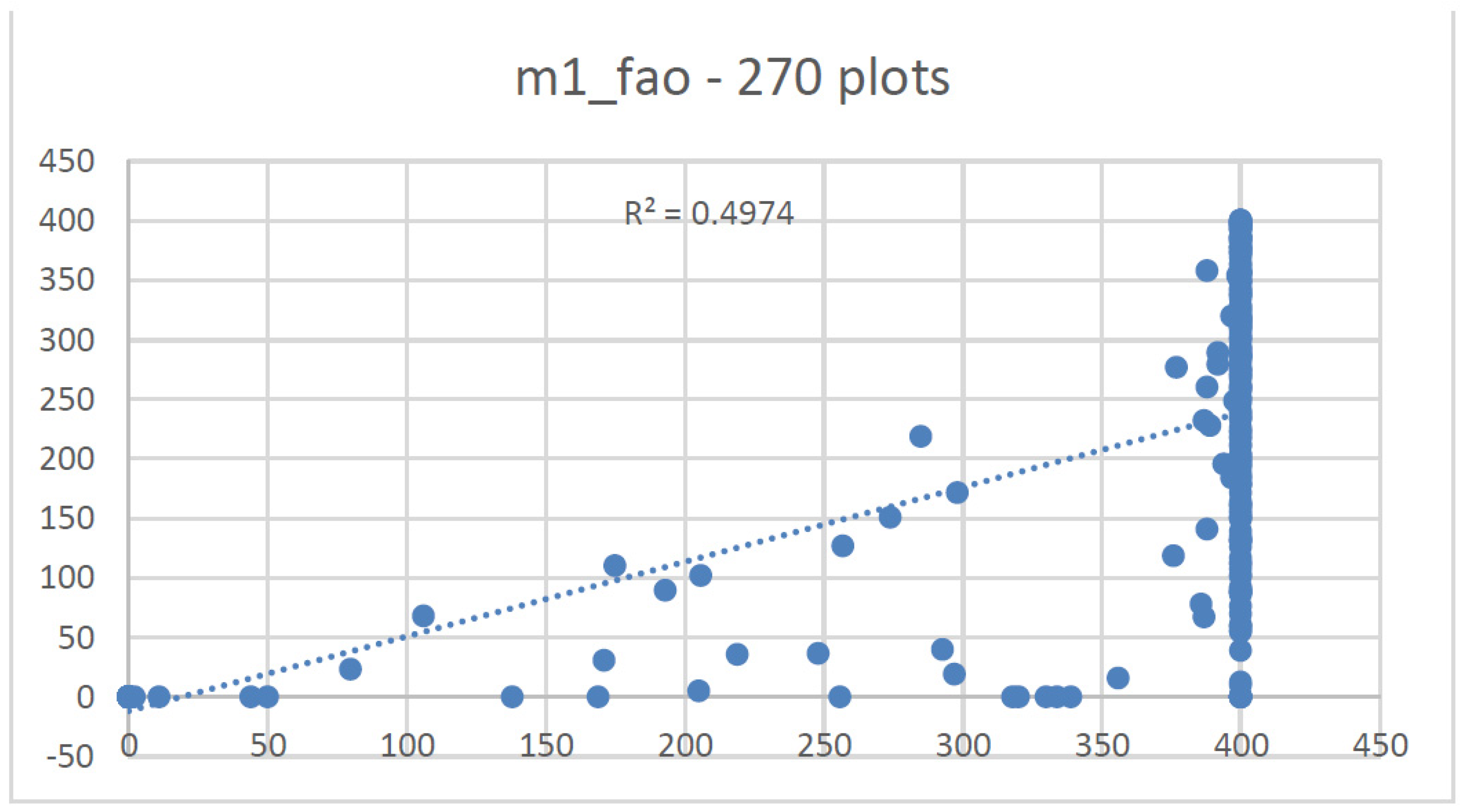
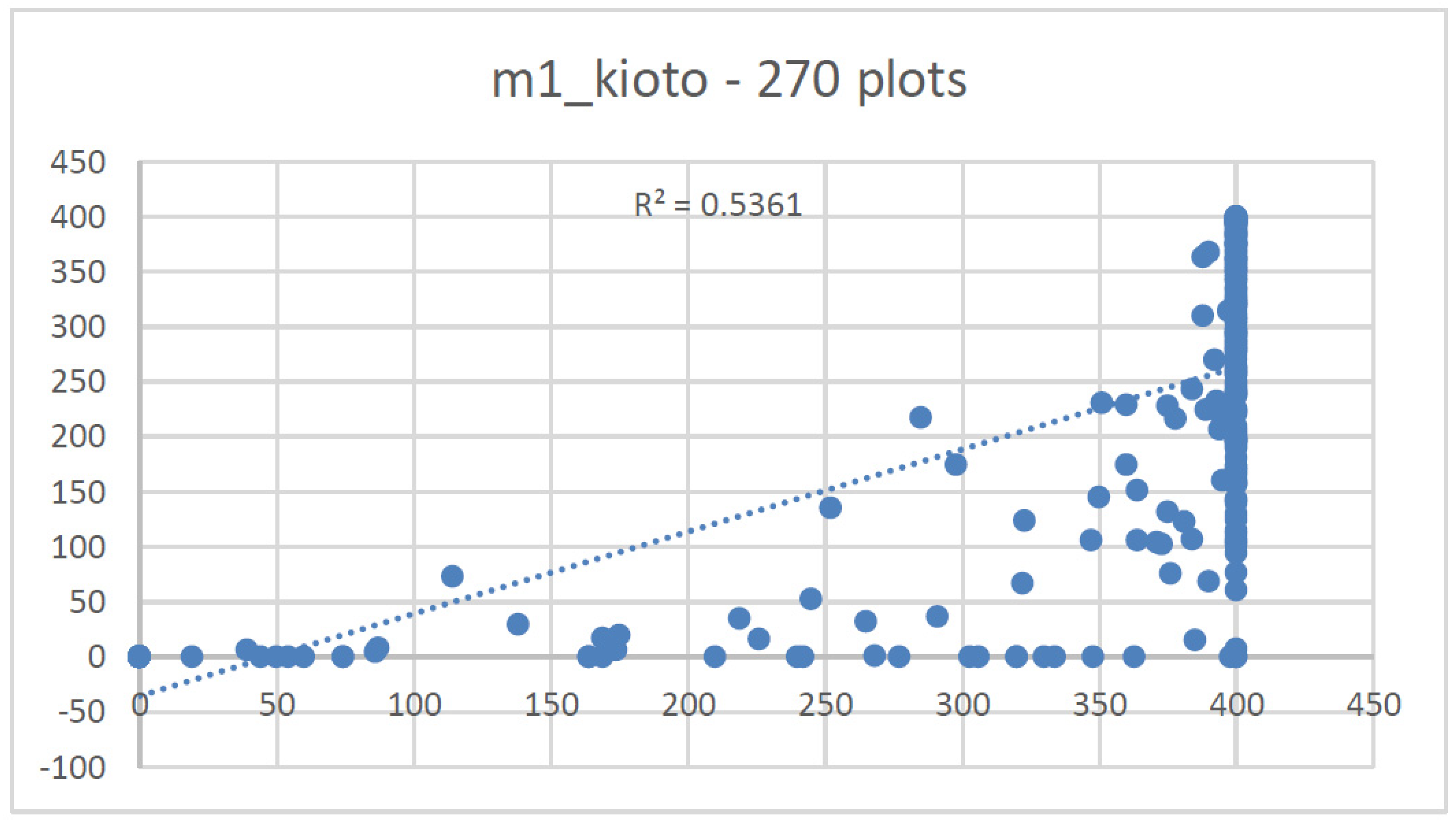
| Method 1 | Eysn et al., 2010, 2011, 2012 Sakcov and Kardos, 2014 [50,51,52,53] | The first method is based on a triangular grid such that each point representing a tree is the vertex of one of the triangles. Such a triangular grid can be created using the Delauney triangulation method. Irregular polygons created during a segmentation process were used to represent the individual trees of 5 m and higher. The areas for which percent cover is calculated (“Convex Hull”) were created based on groups of trees (three each) defined by the vertices of the triangles. |
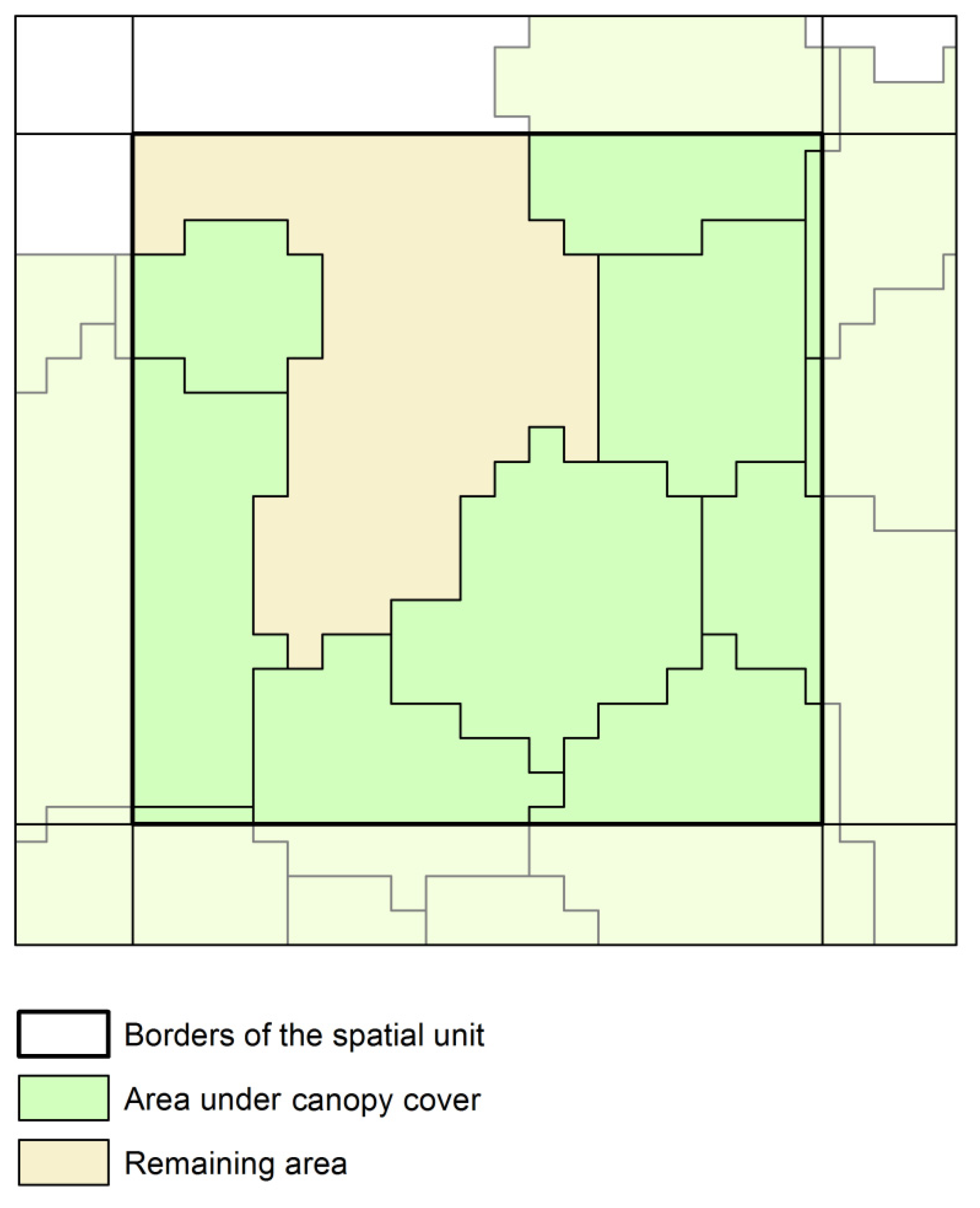
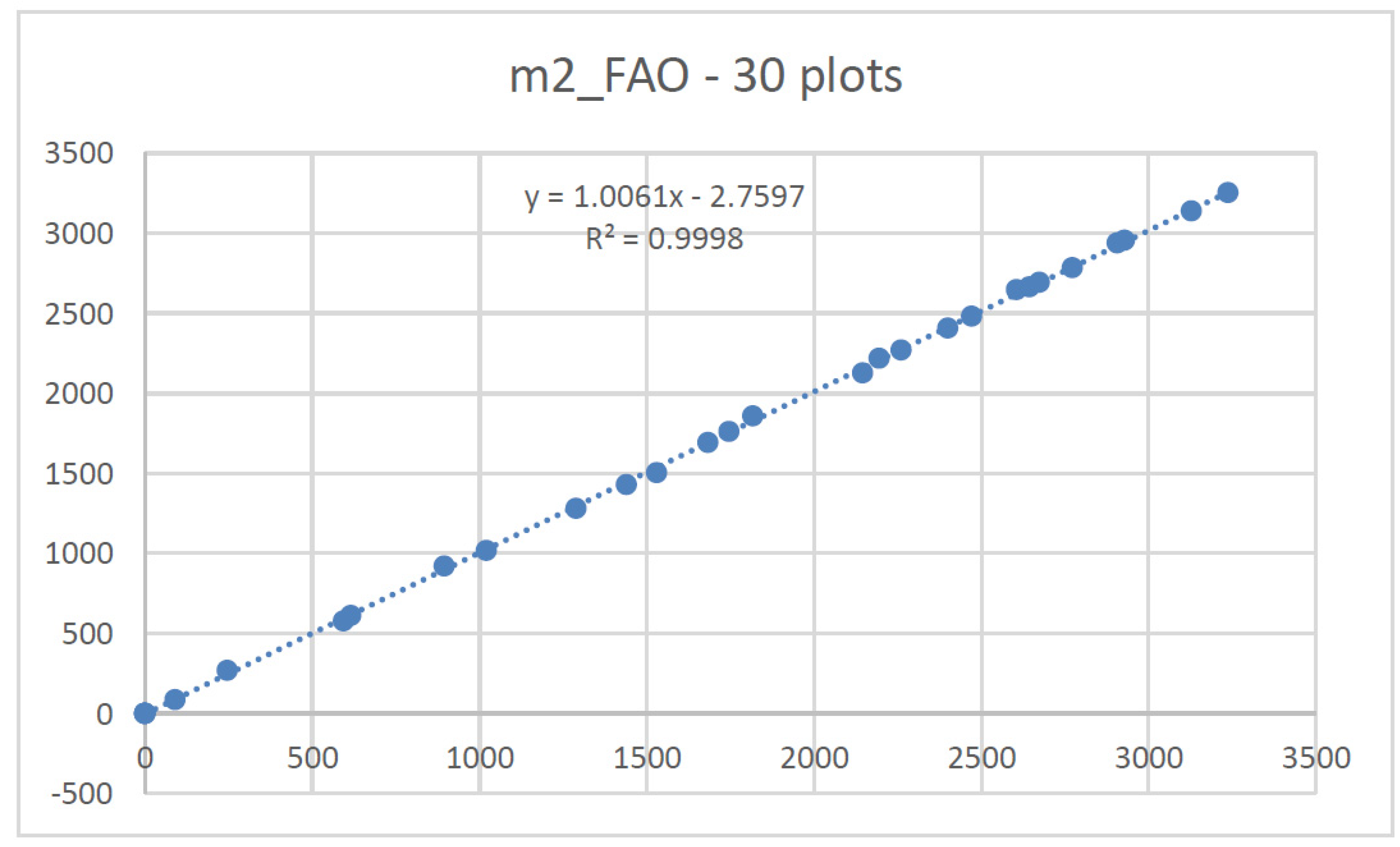
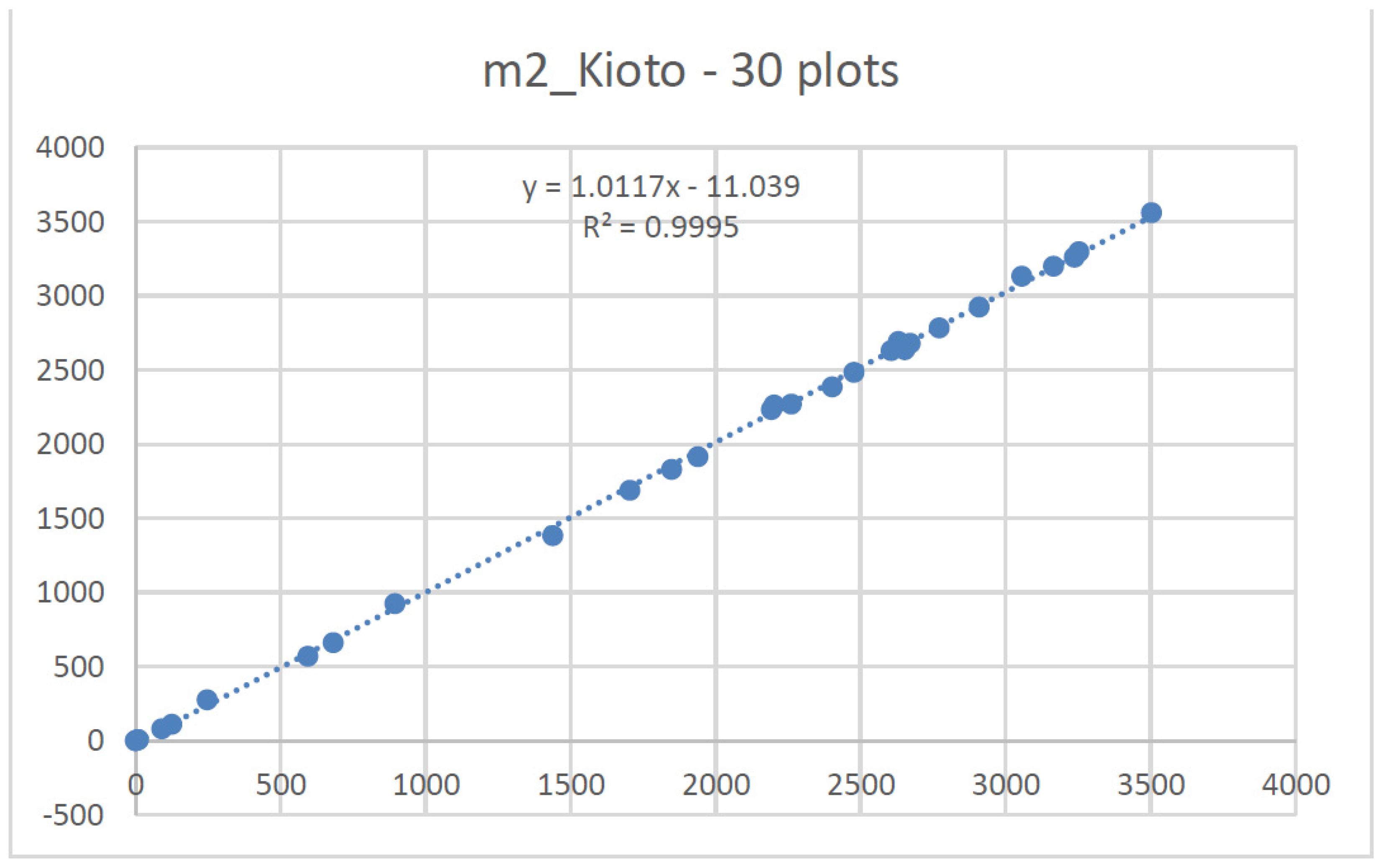
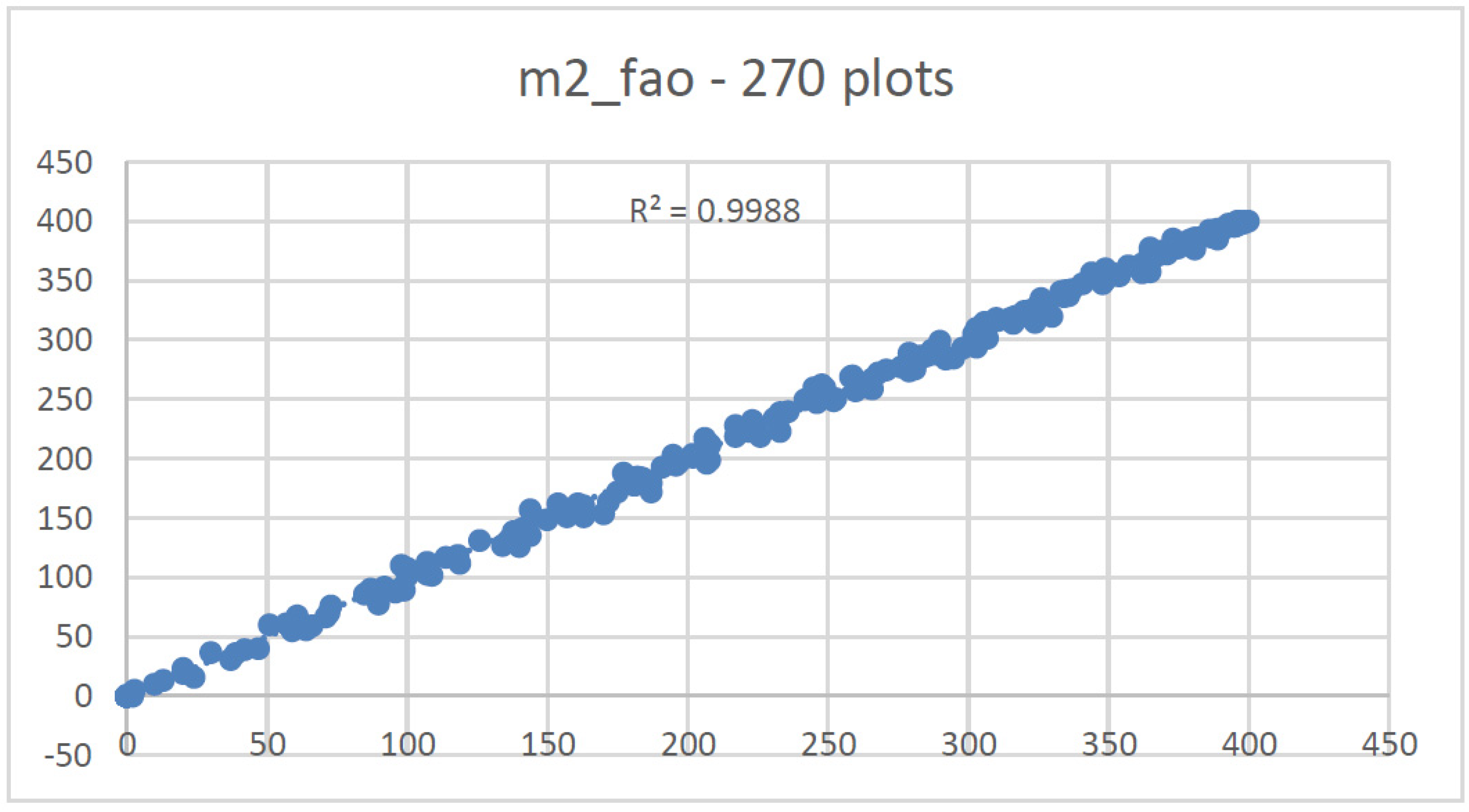
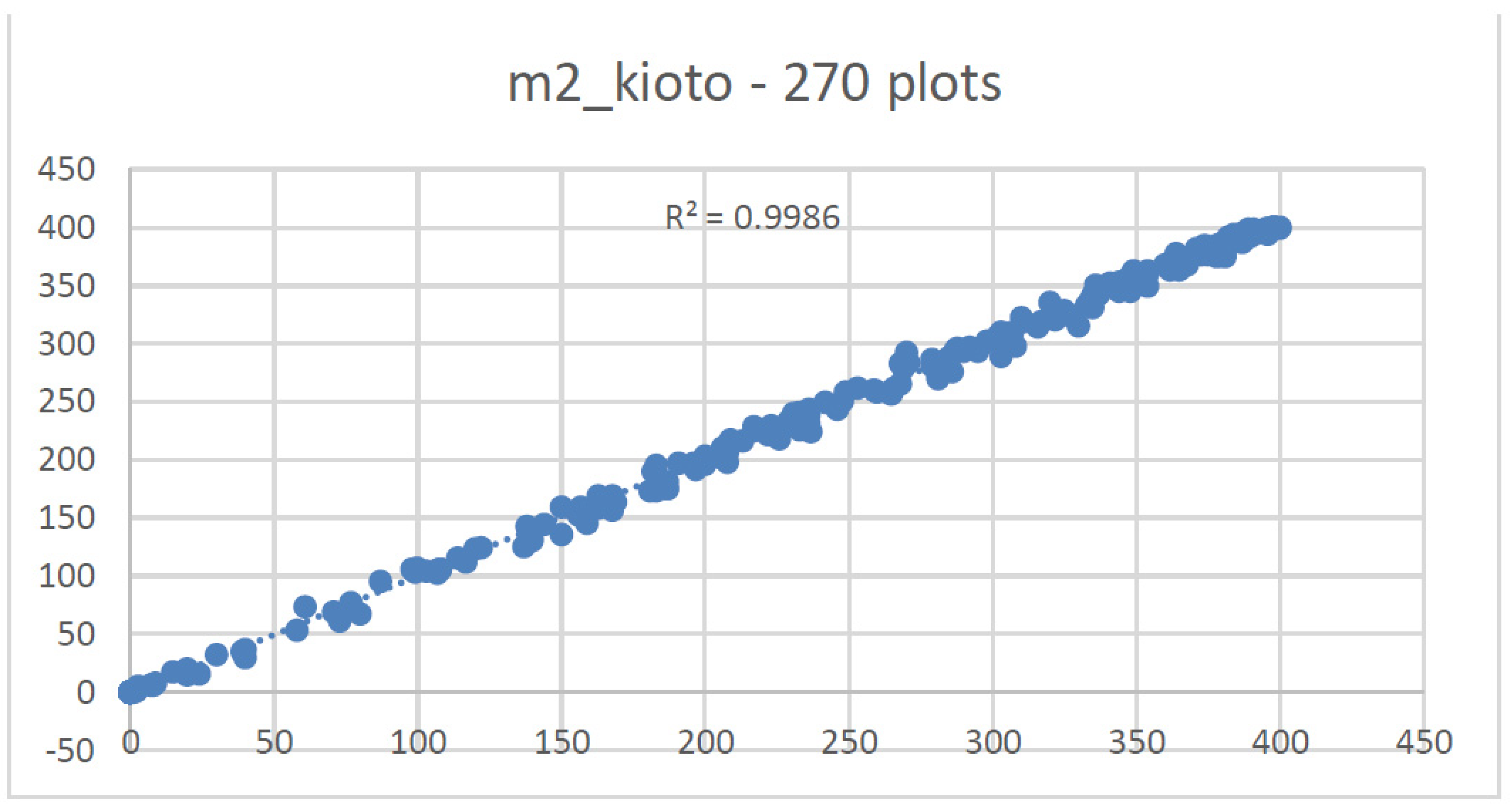
| Method 2 | Straub et al., 2008 [54] | The second method uses only the polygons representing individual tree crowns from the segmentation |
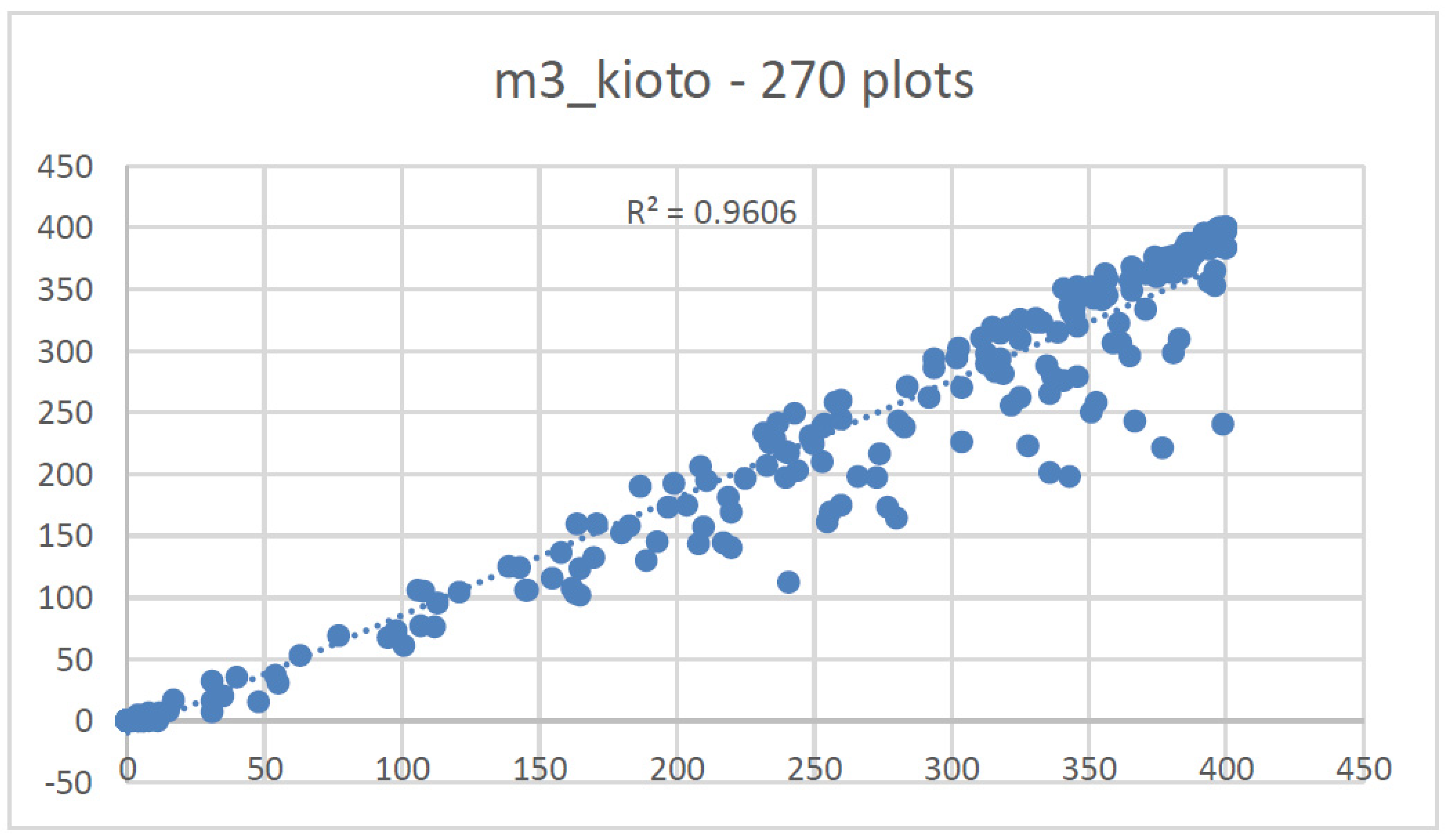
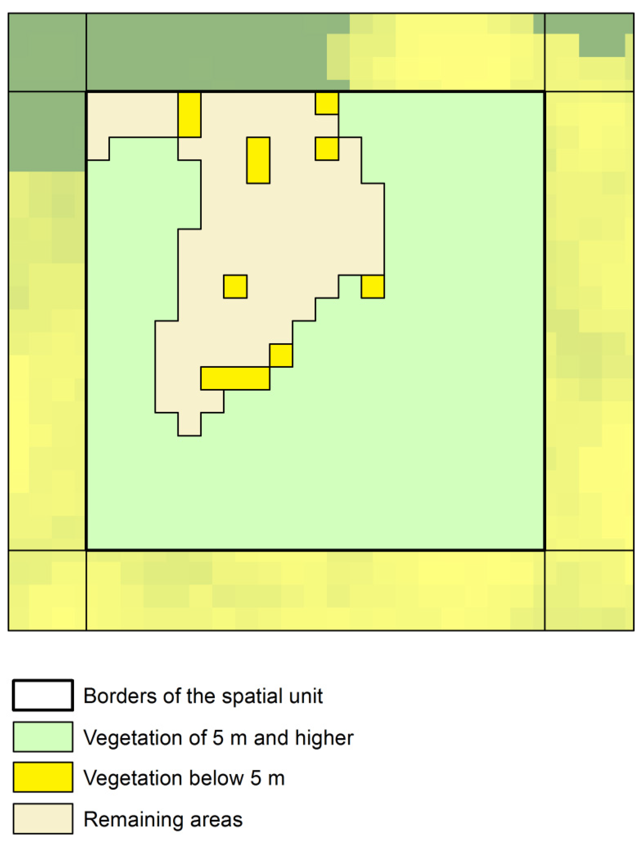
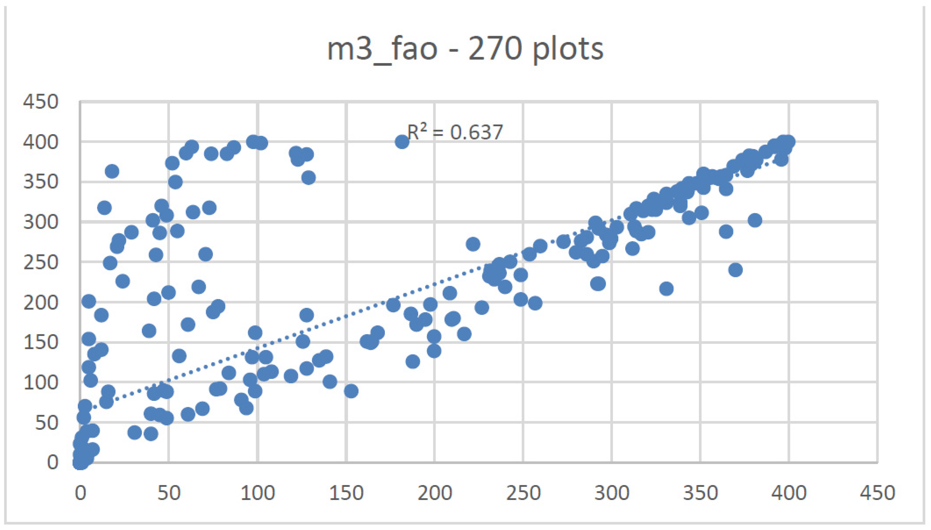
| Method 3 | Wang et al., 2007, 2007, 2008 [27,28,29] | The third method uses only the pixels representing forest vegetation with a height of at least 5 m on the Canopy Height Model |
| Definition | Method 1 | Method 2 | Method 3 | Reference |
|---|---|---|---|---|
| 270 test plots FAO/UN | ||||
| Forest plots | 214 | 187 | 167 | 181 |
| Overall accuracy | 87.8% | 97.8% | 94.8% | n/a |
| Kappa | 0.69 | 0.95 | 0.89 | n/a |
| Commission | 18.2% | 3.3% | n/a | n/a |
| Omission | n/a | n/a | 7.7% | n/a |
| 270 test plots UNFCCC | ||||
| Forest plots | 232 | 196 | 198 | 194 |
| Overall accuracy | 84% | 97.4% | 96.7% | n/a |
| Kappa | 0.55 | 0.94 | 0.92 | n/a |
| Commission | 22.8% | 3.7% | 4.8% | n/a |
| Omission | n/a | n/a | n/a | n/a |
| 30 test plots FAO/UN | ||||
| Forest plots | 25 | 23 | 21 | 23 |
| Overall accuracy | 93.3% | 100% | 93.3% | n/a |
| Kappa | 0.79 | 1 | 0.83 | n/a |
| Commission | 8.7% | 0% | n/a | n/a |
| Omission | n/a | 0% | 8.7% | n/a |
| 30 plots UNFCCC | ||||
| Forest plots | 28 | 23 | 23 | 23 |
| Overall accuracy | 83.3% | 100% | 100% | n/a |
| Kappa | 0.38 | 1 | 1 | n/a |
| Commission | 21.7% | 0% | 0% | n/a |
| Omission | n/a | 0% | 0% | n/a |
| Definition | Method 1 | Method 2 | Method 3 |
|---|---|---|---|
| 270 test plots FAO/UN | |||
| MBE | 123.87 | −0.76 | −33.90 |
| RMSE% | 97.8% | 3.0% | 55.8% |
| MAE% | 70.3% | 2.1% | 27.3% |
| R2 | 0.50 | 0.998 | 0.64 |
| 270 test plots UNFCCC | |||
| MBE | 115.31 | −1.10 | 20.34 |
| RMSE% | 79.3% | 3.0% | 18.4% |
| MAE% | 57.8% | 2.1% | 10.4% |
| R2 | 0.54 | 0.99 | 0.96 |
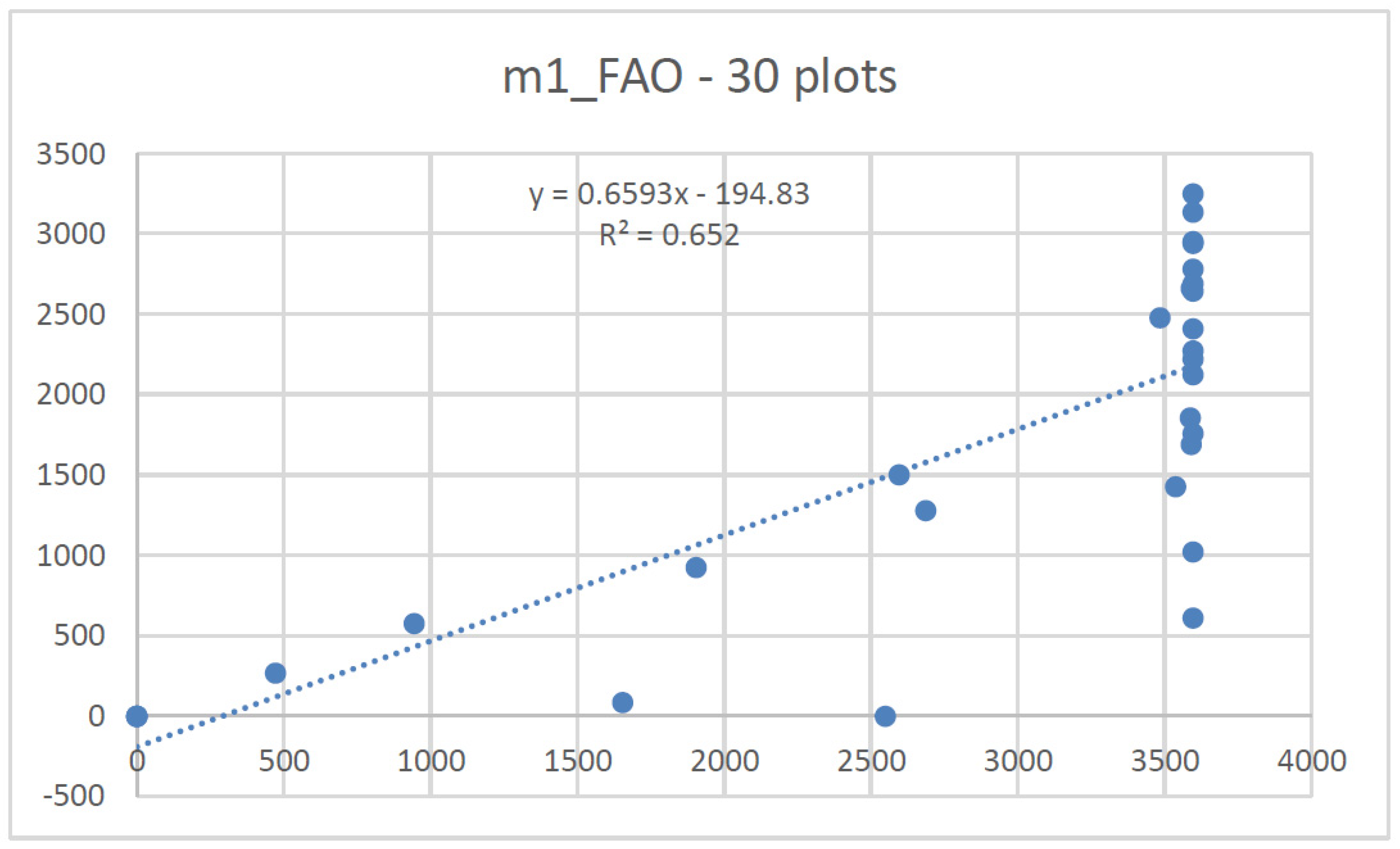
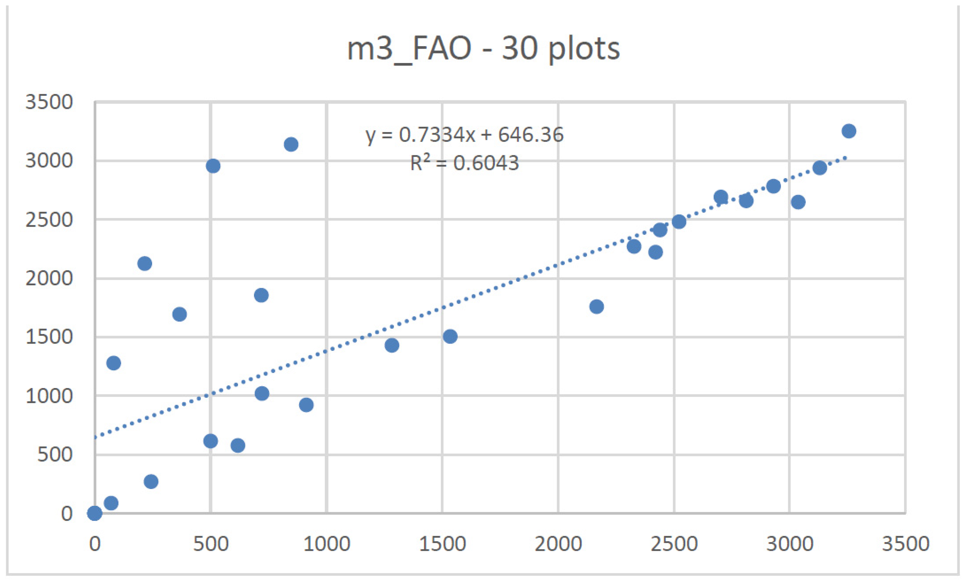
| 30 test plots FAO/UN | |||
| MBE | 1114.83 | −6.80 | −305.07 |
| RMSE% | 86.2% | 1.1% | 51.4% |
| MAE% | 70.3% | 0.9% | 26.6% |
| R2 | 0.65 | 0.99 | 0.60 |
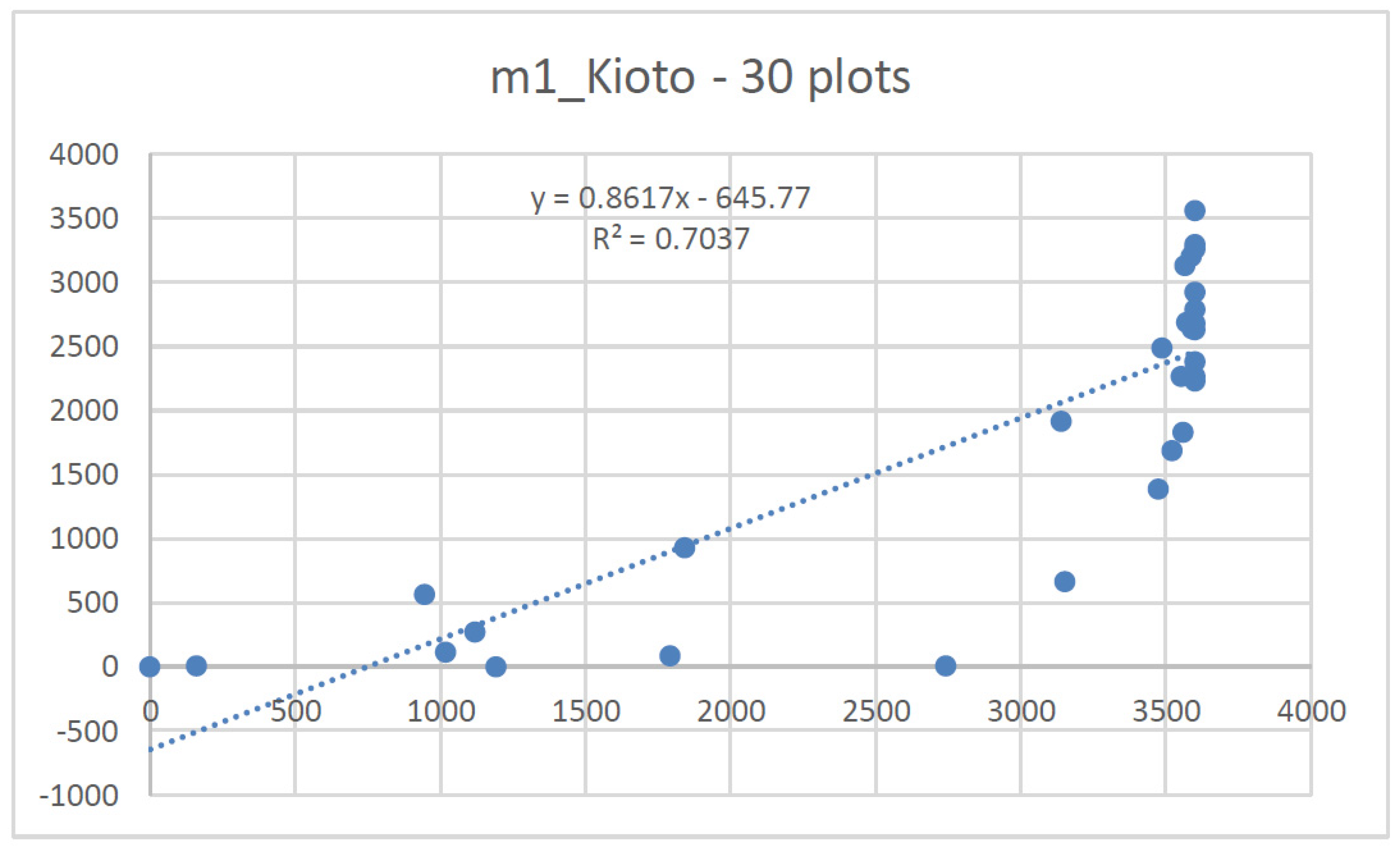
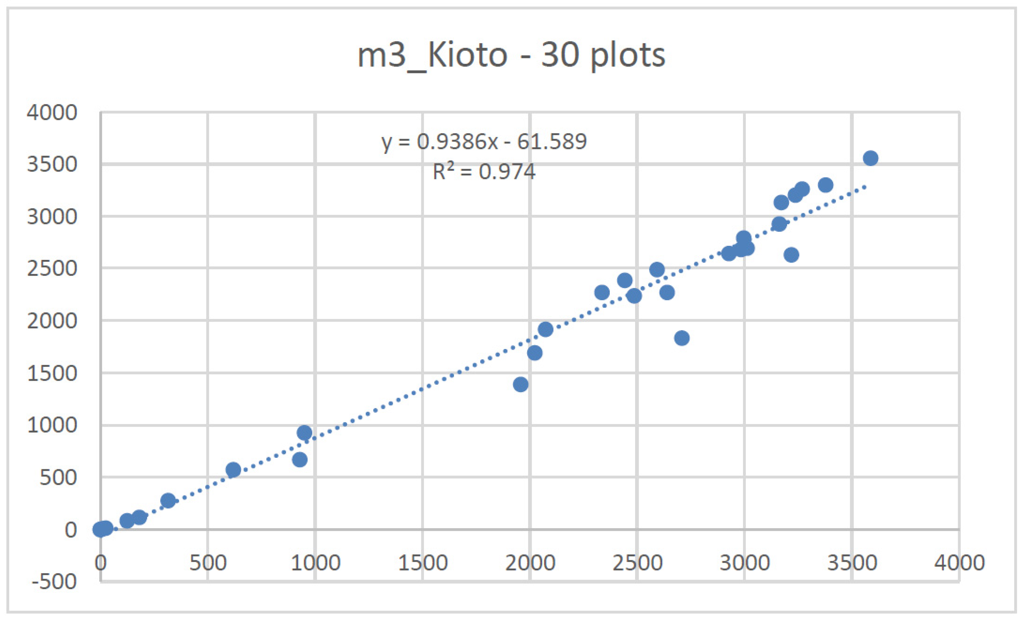
| 30 test plots UNFCCC | |||
| MBE | 1037.83 | −9.87 | 183.03 |
| RMSE% | 68.7% | 1.7% | 15.4% |
| MAE% | 57.8% | 1.3% | 10.2% |
| R2 | 0.70 | 0.99 | 0.97 |
Publisher’s Note: MDPI stays neutral with regard to jurisdictional claims in published maps and institutional affiliations. |
© 2021 by the authors. Licensee MDPI, Basel, Switzerland. This article is an open access article distributed under the terms and conditions of the Creative Commons Attribution (CC BY) license (https://creativecommons.org/licenses/by/4.0/).
Share and Cite
Hycza, T.; Kamińska, A.; Stereńczak, K. The Use of Remote Sensing Data to Estimate Land Area with Forest Vegetation Cover in the Context of Selected Forest Definitions. Forests 2021, 12, 1489. https://doi.org/10.3390/f12111489
Hycza T, Kamińska A, Stereńczak K. The Use of Remote Sensing Data to Estimate Land Area with Forest Vegetation Cover in the Context of Selected Forest Definitions. Forests. 2021; 12(11):1489. https://doi.org/10.3390/f12111489
Chicago/Turabian StyleHycza, Tomasz, Agnieszka Kamińska, and Krzysztof Stereńczak. 2021. "The Use of Remote Sensing Data to Estimate Land Area with Forest Vegetation Cover in the Context of Selected Forest Definitions" Forests 12, no. 11: 1489. https://doi.org/10.3390/f12111489
APA StyleHycza, T., Kamińska, A., & Stereńczak, K. (2021). The Use of Remote Sensing Data to Estimate Land Area with Forest Vegetation Cover in the Context of Selected Forest Definitions. Forests, 12(11), 1489. https://doi.org/10.3390/f12111489