The Effects of Combining the Variables in Allometric Biomass Models on Biomass Estimates over Large Forest Areas: A European Beech Case Study

Abstract

Effective initiatives for forest-based mitigation of climate change rely on continuous efforts to improve the estimation of forest biomass. Allometric biomass models, which are nonlinear models that predict aboveground biomass (AGB) as a function of diameter at breast height (D) and tree height (H), are typically used in forest biomass estimations. A combined variable D²H may be used instead of two separate predictors. The Q-ratio (i.e., the ratio between the parameter estimates of D and parameter estimates of H, in a separate variable model) was proposed recently as a measure to guide the decision on whether D and H can be safely combined into D²H, being shown that the two model forms are similar when Q = 2.0. Here, using five European beech (Fagus sylvatica L.) biomass datasets (of different Q-ratios ranging from 1.50 to 5.05) and an inventory dataset for the same species, we investigated the effects of combining the variables in allometric models on biomass estimation over large forest areas. The results showed that using a combined variable model instead of a separate variable model to predict biomass of European beech trees resulted in overestimation of mean AGB per hectare for Q > 2.0 (i.e., by 6.3% for Q = 5.05), underestimation for Q < 2.0 (i.e., by –3.9% for Q = 1.50), whereas for Q = 2.03, the differences were minimum (0.1%). The standard errors of mean AGB per hectare were similar for Q = 2.03 (differences up to 0.2%), and the differences increased with the Q-ratio, by up to 10.2% for Q = 5.05. Therefore, we demonstrated for European beech that combining the variables in allometric biomass models when Q ≠ 2.0 resulted in biased estimates of mean AGB per hectare and of uncertainty.

1. Introduction

The policies on forest-based mitigation of climate change cannot be successfully implemented without a rigorous quantification of the forest carbon stock and/or stock change [1,2,3,4,5]. Usually, forest carbon is not estimated directly; the forest biomass is first quantified and then a species-specific biomass-to-carbon ratio is used to transform biomass to carbon [3]. Therefore, the real challenge is the estimation of forest biomass [6]. Forest biomass estimation relies, in many cases, on the use of allometric biomass models [7], which are nonlinear regression models predicting tree aboveground biomass (AGB) as a function of diameter at breast height (D) and/or tree height (H) [8,9]. These models are then applied to a sample of plots, which may involve remote sensing data, to obtain a statistical parameter of mean biomass per unit of forest area [3,10].

The addition of H as a predictor variable in allometric biomass models was shown to improve the biomass prediction [11,12] and reduce the dependence of allometric models on sites [13]. However, the dependence on tree species was only marginally reduced when including H [13], although ‘wood density’ as an additional predictor of D and H was shown to significantly reduce dependence on species [14].

Correlation of D and H, although strong, is never perfect; the relationship between D and H is affected by genotype, age, tree competition, and environmental conditions [15,16]. If the correlation would be perfect (i.e., r = 1.0), the addition of H in allometric models would be redundant. It is to be expected that for trees of similar D, the variability in H will cause some variability in AGB. Therefore, the addition of H as a predictor of biomass explains the variability in AGB produced by variability in H for trees of any given D.

The variables D and H are commonly used separately in allometric models to predict AGB. Although weighting for heteroscedasticity of residuals in nonlinear models is easily implemented in statistical software routines, a logarithmic transformation of all variables is often used to stabilize the variance and to linearize the model:

$$\ln \left(AGB\right)={\beta }_{10}+{\beta }_{11}\cdot \ln \left(D\right)+{\beta }_{12}\cdot \ln \left(H\right)+{\epsilon }_1$$

(1)

Nevertheless, because variables D and H are correlated, there is inherently a degree of collinearity in allometric biomass models when both D and H are used as individual predictors of biomass [12]. Alternatively, to avoid the negative effects of collinearity [17], the variables D and H can be combined into a single predictor variable D²H, being justified by the proportionality between AGB and the cylinder of diameter, D, and height, H [14]:

$$\ln \left(AGB\right)={\beta }_{20}+{\beta }_{21}\cdot \ln \left(D^{2}H\right)+{\epsilon }_2$$

(2)

The combined variable model contains a lower number of parameters, and, therefore, a lower number of variances and covariances to be estimated. Equation (2) can be fitted with only a single parameter, assuming isometry between the predictor variable and the predicted AGB (i.e., if ${\beta }_{21}=1$) [14].

However, combining the variables D and H into D²H is not that harmless. Dutcă et al. [18] showed that combining the variables into D²H can affect the accuracy of biomass prediction under certain conditions. They proposed a practical measure, the Q-ratio:

$$Q=\frac{{\widehat{\beta }}_{11}}{{\widehat{\beta }}_{12}}$$

(3)

where ${\widehat{\beta }}_{11}$ and ${\widehat{\beta }}_{12}$ are the parameter estimates from Equation (1), to guide the decision as to whether D and H may be combined into D²H without the adverse effects of loss in biomass prediction accuracy. The authors showed that there is no preference in using a log-transformation or a weighted nonlinear approach to fit the allometric model (Equation (1)) in order to calculate the Q-ratio (Equation (3)), since the differences in estimated Q-ratio were minor [18]. The combined variable model (Equation (2)) is the equivalent of the separate variable model (Equation (1)), when Q = 2.0, and, therefore, the combined variable model can be safely used instead of separate variable model when Q = 2.0. They demonstrated that the combined variable model became less efficient in predicting AGB as the Q-ratio deviated from 2.0 [18]. Since Dutcă et al. [18] investigated the effects at the level of allometric models only, and it is essential to investigate the effects of using a combined variable to predict biomass over large forest areas, when the Q-ratio deviates from 2.0.

Therefore, in this paper we investigated the effects of using a combined variable model (Equation (2)) instead of a separate variable model (Equation (1)), under different levels of Q-ratios, to predict biomass for large European beech forest areas.

2. Materials and Methods

2.1. Data

2.1.1. Calibration Datasets

The calibration data were used to fit the allometric biomass models to predict the biomass of individual trees within the inventory dataset. Since the aim of our study was to investigate the effects of different levels of Q-ratios [18] on using the combined variable to predict the biomass over large forest areas, we derived five biomass datasets having different Q-ratios. We started from a large biomass dataset [19] and selected only European beech (Fagus sylvatica L.) trees with D > 5.6 cm to match the starting D-range for the inventory dataset. We obtained a ‘beech dataset’ containing 221 observations.

We further resampled from the ‘beech dataset’, without replacement, a constant number of 100 trees. To each resampled dataset we fitted an allometric model taking the form of Equation (1) and calculated the Q-ratio as in Equation (3). The resampling continued until the Q-ratio was within the following intervals: 1.5 ± 0.05, 2 ± 0.05, 3 ± 0.05, 4 ± 0.05 and 5 ± 0.05. Therefore, we obtained five biomass (i.e., calibration) datasets, each containing 100 trees, but having a different Q-ratio. The actual Q-ratios and other characteristics for each calibration dataset used in this study are presented in

Table 1. The characteristics of the calibration datasets.

Dataset Name	Q-Ratio	Sample Size	D-Range (cm)	H-Range (m)	AGB-Range (kg)
Q1	1.50	100	5.6–60.1	7.91–35.80	8.3–3456.6
Q2	2.03	100	5.6–86.3	8.54–40.30	8.3–8447.1
Q3	3.03	100	6.1–86.3	8.20–40.30	10.1–8447.1
Q4	4.03	100	6.0–86.3	5.64–40.30	11.3–8447.1
Q5	5.05	100	6.2–86.3	9.39–40.30	11.4–8447.1

.

2.1.2. Inventory Dataset

The inventory dataset was selected from Romanian National Forest Inventory (NFI). Out of 5036 sample plots within the NFI network, we selected all plots containing only beech (Fagus sylvatica L.) trees. A total of 298 sample plots were identified and considered for the study. The diameter at breast height (D) range was between 5.6 and 101.0 cm; the H range was between 3.0 and 49.3 m.

European beech is the most important tree species in Romania, covering 2.11 million ha, according to the National Forest Inventory. Because of the widespread distribution of European beech in Romania, it is the best-suited species [20,21].

The Romanian NFI uses a 4 by 4 km grid in the mountain area [21] where the beech trees grow. Therefore, each plot is representative of a forest area of 16 km², and the 298 plots correspond to 476.8 thousand hectares of forest. Each sample plot consists of two sub-plots in which trees of different sizes are measured for D (with a precision of 1 mm) and H (with a precision of 1 cm). In a smaller circular sub-plot (200 m²) all trees with a diameter at breast height (D) between 5.6 and 28.5 cm are measured. In a larger sub-plot (circular sub-plot of 500 m², concentrical to the small sub-plot) all trees with D > 28.5 cm are measured [22].

2.2. Data Analysis

2.2.1. Fitting Allometric Models to Calibration Datasets

To each calibration dataset (i.e., Q1 to Q5, Table 1) we fitted two allometric models, taking the form of:

(a)

separate variable model (Equation (1));

(b)

combined variable model (Equation (2)).

2.2.2. Prediction of Biomass

For every tree in every plot within the inventory dataset, the AGB was predicted using

(a)

the separate variable model:

$${\widehat{AGB}}_{ij}{}^s=\exp \left({\widehat{\beta }}_{10}\right)\cdot D_{ij}{}^{{\widehat{\beta }}_{11}}\cdot H_{ij}{}^{{\widehat{\beta }}_{12}}\cdot \exp \left(\frac{RS{E}_1{}^2}{2}\right)$$

(4)

where ${\widehat{\beta }}_{10}$, ${\widehat{\beta }}_{11}$, and ${\widehat{\beta }}_{12}$ are the parameter estimates of Equation (1) fitted to Datasets Q1–Q5; $D_{ij}$ is the diameter at breast height of the ith tree from the jth plot in the inventory dataset; $H_{ij}$ is the height of the ith tree from the jth plot in the inventory dataset; RSE₁ is the residual standard error of Equation (1) that was used to calculate the back transformation correction factor [23].

(b)

the combined variable model:

$${\widehat{AGB}}_{ij}{}^c=\exp \left({\widehat{\beta }}_{20}\right)\cdot {(D^2{H}_{ij})}^{{\widehat{\beta }}_{21}}\cdot \exp \left(\frac{RS{E}_2{}^2}{2}\right)$$

(5)

where ${\widehat{\beta }}_{20}$ and ${\widehat{\beta }}_{21}$ are the parameter estimates of Equation (2); $D^2{H}_i$ is the combined predictor variable for the ith tree in the jth plot in the inventory dataset (it was calculated by multiplication of squared D with H); RSE₂ is the residual standard error of Equation (2); exp(RSE₂²/2) is the correction factor [23].

For each plot, the individual tree predictions were added and then extrapolated per hectare. We used an expansion factor of 50 for the small subplot (i.e., of 200 m², where the trees with 5.6 ≤ D ≤ 28.5 cm were measured) and a factor of 20 for the large subplot (i.e., of 500 m², where the trees with D > 28.5 cm were measured):

$${\widehat{AGB}}_j{}^s=50\cdot {{\displaystyle \sum }}_{i=1}^{n_{j1}}{\widehat{AGB}}_i{{}^s}^{\left(\mathrm{small}\mathrm{subplot}\right)}+20\cdot {{\displaystyle \sum }}_{\mathrm{i}=1}^{n_{j2}}{\widehat{AGB}}_i{{}^s}^{\left(\mathrm{large}\mathrm{subplot}\right)}$$

(6)

$${\widehat{AGB}}_j{}^c=50\cdot {{\displaystyle \sum }}_{i=1}^{n_{j1}}{\widehat{AGB}}_i{{}^c}^{\left(\mathrm{small}\mathrm{subplot}\right)}+20\cdot {{\displaystyle \sum }}_{i=1}^{n_{j2}}{\widehat{AGB}}_i{{}^c}^{\left(\mathrm{large}\mathrm{subplot}\right)}$$

(7)

where ${\widehat{AGB}}_i{}^s$ is the predicted AGB of the ith tree based on separate variable model (Equation (4)) from either the small or the large subplot; ${\widehat{AGB}}_i{}^c$ is the predicted AGB of the ith tree based on combined variable model (Equation (5)) from either the small or the large subplot; n_j1 is the total number of measured trees in the small subplot; n_j2 is the total number of measured trees in the large subplot.

Assuming negligible uncertainty due to allometric model predictions [24,25] and an equal probability sample, the population mean AGB per hectare (i.e., ${\widehat{\mu }}^s$ based on the separate variable model and ${\widehat{\mu }}^c$ based on the combined variable model) and the standard error of the mean (i.e., $SE\left({\widehat{\mu }}^s\right)$ and $SE\left({\widehat{\mu }}^c\right)$) were estimated using a simple expansion estimator [26,27]. Therefore, under simple expansion estimation, the uncertainty that originated in allometric biomass models (e.g., variance-covariance matrix and residual variance) was not included:

$${\widehat{\mu }}^s=\frac{1}{n}{{\displaystyle \sum }}_{j=1}^n{\widehat{AGB}}_j{}^s$$

(8)

$${\widehat{\mu }}^c=\frac{1}{n}{{\displaystyle \sum }}_{j=1}^n{\widehat{AGB}}_j{}^c$$

(9)

$$SE\left({\widehat{\mu }}^s\right)=\sqrt{\frac{1}{n\left(n-1\right)}{\displaystyle \sum }_{j=1}^n{\left({\widehat{AGB}}_j{}^s-{\widehat{\mu }}^s\right)}^2}$$

(10)

$$SE\left({\widehat{\mu }}^c\right)=\sqrt{\frac{1}{n\left(n-1\right)}{\displaystyle \sum }_{j=1}^n{\left({\widehat{AGB}}_j{}^c-{\widehat{\mu }}^c\right)}^2}$$

(11)

where ${\widehat{AGB}}_j{}^s$ is the predicted AGB of the j^th plot from Equation (6); ${\widehat{AGB}}_j{}^c$ is the predicted AGB of the jth plot from Equation (7); n is the total number of plots.

We further investigated the differences between the estimates based on separate variable models (Equation (4)) and estimates from combined variable models (Equation (5)) at the level of (i) individual tree predictions and (ii) plot level estimates. Bland–Altman plots [28,29] were developed to report the mean difference (or bias) (MD) and the limits of agreement (LoA) of estimates derived from the two model forms. At the level of individual trees, the MD_tree and LoA_tree were calculated as:

$$M{D}_{tree}=\frac{1}{N}{\displaystyle \sum }_{i=1}^N({\widehat{AGB}}_i{}^c-{\widehat{AGB}}_i{}^s)$$

(12)

$$Lo{A}_{tree}=1.96\cdot \sqrt{\frac{1}{N-1}{\displaystyle \sum }_{i=1}^N{\left[\left({\widehat{AGB}}_i{}^c-{\widehat{AGB}}_i{}^s\right)-M{D}_{tree}\right]}^2}$$

(13)

where ${\widehat{AGB}}_i{}^s$ is the predicted AGB of the ith tree in the inventory dataset based on the separate variable model (Equation (4)); ${\widehat{AGB}}_i{}^c$ is the predicted AGB of the ith tree in the inventory dataset based on the combined variable model (Equation (5)); N is the total number of trees in the inventory dataset.

At the level of individual plots, the MD_plot and LoA_plot were calculated as:

$$M{D}_{plot}=\frac{1}{n}{\displaystyle \sum }_{j=1}^n({\widehat{AGB}}_j{}^c-{\widehat{AGB}}_j{}^s)$$

(14)

$$Lo{A}_{plot}=1.96\cdot \sqrt{\frac{1}{n-1}{\displaystyle \sum }_{j=1}^n{\left[\left({\widehat{AGB}}_j{}^c-{\widehat{AGB}}_j{}^s\right)-M{D}_{plot}\right]}^2}$$

(15)

where ${\widehat{AGB}}_j{}^c$ is the estimated AGB per hectare of the j^th plot (Equation (7)), which used the combined variable model to predict the AGB of individual trees; ${\widehat{AGB}}_j{}^s$ is the estimated AGB per hectare of the j^th plot (Equation (6)), which used the separate variable model to predict the AGB of individual trees; n is the total number of plots.

2.3. Data Processing

The processing and analysis of the data were performed in R [30] with the RStudio interface [31].

3. Results

3.1. The Effects at the Level of Large Forest Area Estimates

The estimates of mean AGB per hectare and their standard errors are presented in

Table 2. The estimates of mean AGB per hectare and of SE, in Mg·ha–1, by model form and dataset. ${\widehat{\mu }}^s$ is the mean AGB per hectare based on the separate variable model, Equation (8); ${\widehat{\mu }}^c$ is the mean AGB per hectare based on the separate variable model, Equation (9); $SE\left({\widehat{\mu }}^s\right)$ is the standard error of ${\widehat{\mu }}^s$, Equation (10); $SE\left({\widehat{\mu }}^c\right)$ is the standard error of ${\widehat{\mu }}^c$, Equation (11). The relative difference was calculated as the ratio between the difference (i.e., the estimates of the combined variable model minus the estimates of the separate variable model) and the estimates based on the separate variable model, multiplied by 100.

Dataset	Q-Ratio	$\mathbf{Mean}\mathbf{AGB}\mathbf{per}\mathbf{Hectare}\left(\widehat{\mathit{\mu }}\right)$			SE$\mathbf{of}\mathbf{the}\mathbf{Mean}\left(\mathit{S}\mathit{E}\left(\widehat{\mathit{\mu }}\right)\right)$
		$$\begin{gathered} {\widehat{\mathit{\mu }}}^{\mathit{s}} \\ (\mathbf{Mg}·{\mathbf{ha}}^{-1}) \end{gathered}$$	$$\begin{gathered} {\widehat{\mathit{\mu }}}^{\mathit{c}} \\ (\mathbf{Mg}·{\mathbf{ha}}^{-1}) \end{gathered}$$	Relative Difference (%)	$$\begin{gathered} \mathit{S}\mathit{E}\left({\widehat{\mathit{\mu }}}^{\mathit{s}}\right) \\ (\mathbf{Mg}·{\mathbf{ha}}^{-1}) \end{gathered}$$	$$\begin{gathered} \mathit{S}\mathit{E}\left({\widehat{\mathit{\mu }}}^{\mathit{c}}\right) \\ (\mathbf{Mg}·{\mathbf{ha}}^{-1}) \end{gathered}$$	Relative Difference (%)
Q1	1.50	289.30	278.09	–3.9	10.54	9.91	–6.0
Q2	2.03	276.71	277.00	0.1	9.84	9.86	0.2
Q3	3.03	287.03	297.63	3.7	10.08	10.66	5.8
Q4	4.03	274.99	290.44	5.6	9.50	10.35	9.0
Q5	5.05	270.28	287.34	6.3	9.19	10.18	10.8

, for the two model forms (i.e., separate variables and combined variables). For Dataset Q2 (Q = 2.03), the difference in mean AGB per hectare between estimates based on combined vs. separate variable models (i.e., ${\widehat{\mu }}^c$ vs. ${\widehat{\mu }}^s$) was the lowest, by approximately 0.1% (Table 2). However, this difference increased as the Q-ratio departed from 2.0. For Q > 2.0, the estimates based on combined variable models were larger than those based on separate variable models, the difference increasing gradually for Datasets Q3, Q4, and Q5 because of the increasing Q-ratio. The largest difference in mean AGB per hectare (i.e., 6.3%, Table 2) was observed for Dataset Q5 (Q = 5.05). For Q < 2.0, the differences were negative. The estimates of mean AGB per hectare based on combined variables were smaller compared to those based on the separate variable model, by 3.9% (Table 2) for Dataset Q1. Therefore, the negative effects of using a combined variable model instead of separate variables were minimal when Q = 2.0 and increased as the Q-ratio departed from the threshold value of 2.0.

The Q-ratio also affected the estimates of uncertainty. The relative difference of SE increased with the Q-ratio (Table 2). For Dataset Q5, the SE increased by more than 10% when using a combined variable model instead of a separate variable model. The SE relative to the mean AGB per hectare (i.e., the coefficient of variation) was between 3.4% and 3.6%.

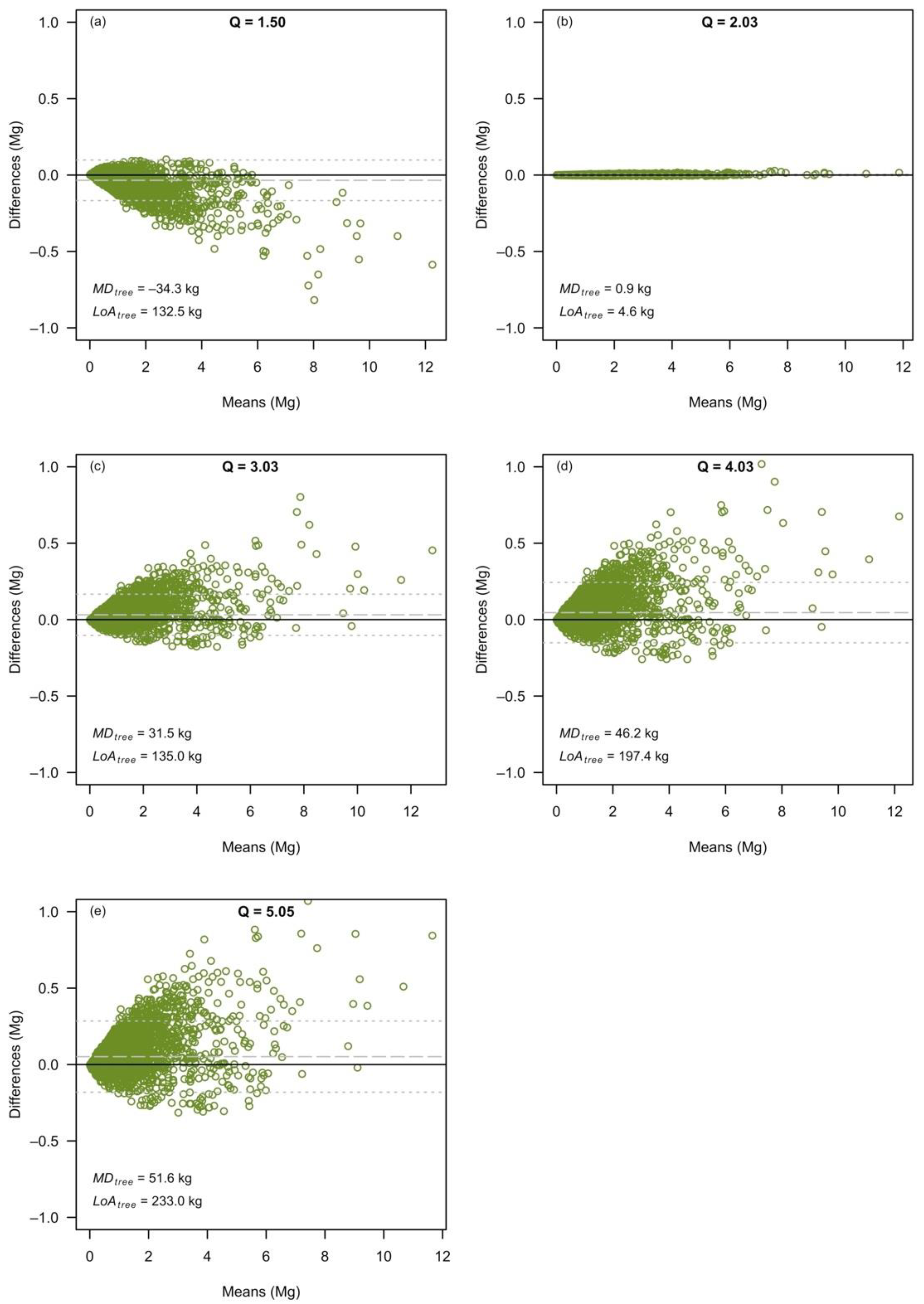
3.2. The Effects at the Level of Individual Tree Predictions

It was confirmed, at the level of individual tree predictions, that the smallest differences between models based on separate variables and models based on combined variables occurred for Dataset Q2 (Q = 2.03, Figure 1b). For Q ≠ 2.0, the smallest differences in absolute values occurred for the smallest trees whereas the largest differences occurred for the largest trees (Figure 1a,c–e). The mean difference (MD_tree), which is the average difference of the predicted biomass per tree, was closest to zero (i.e., unbiased) for Q = 2.03 (i.e., 0.9 kg per tree). However, MD_tree increased for Q > 2.0, up to 51.6 kg per tree for Dataset Q5. Therefore, for Dataset Q5, the combined variable model estimated, on average, a 51.6 kg heavier tree biomass compared with the separate variable model. This large MD_tree was driven by the large differences in large trees, which for Dataset Q5 reached 1357 kg for a tree that had ${\widehat{AGB}}^s$ = 6.37 Mg and ${\widehat{AGB}}^c$ = 7.73 Mg. As can be observed in Figure 1, for small trees, the differences were relatively small and balanced. For Q < 2.0, the MD_tree decreased by up to 34.5 kg per tree (for Q = 1.50). Therefore, for Dataset Q1, the combined variable model predicted, on average, 34.5 kg per tree less compared to the separate variable model.

The limit of agreement (LoA_tree) that indicates how well the two model forms agree in their predictions was lowest for Dataset Q2 (i.e., 4.6 kg). The LoA_tree increased for both Q < 2.0 and Q > 2.0. For Q > 2.0, the LoA_tree increased up to 233.0 kg (for Dataset Q5), while for Q < 2.0, the LoA_tree increased up to 132.5 kg (for Dataset Q1). Therefore, the agreement between predictions of the two model forms was weaker as the Q-ratio departed from 2.0. Although dealing with only a single dataset with Q < 2.0, we conjecture that the differences between separate and combined predictor variables were more strongly affected by the Q-ratio for Q < 2.0. A decrease of 0.5 units in the Q-ratio below the threshold value of 2.0 produced differences that were comparable to those of Q = 3.03 (therefore, one unit above 2.0).

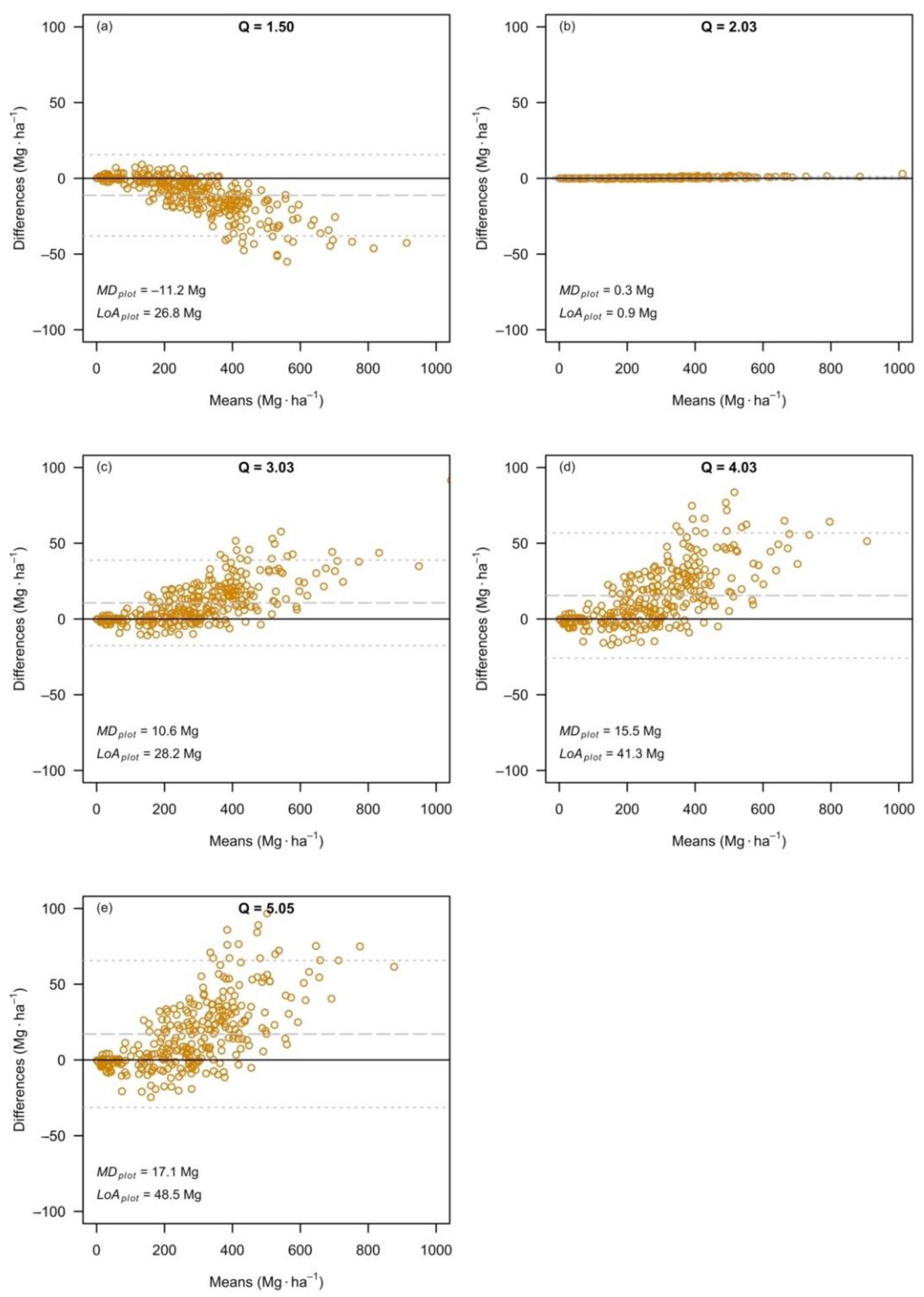
3.3. The Effects at the Level of Plot Estimates

The trends observed at the level of individual tree predictions were replicated at the level of individual plot estimates. This was partly expected because the estimates of plot biomass are based on individual tree predictions. However, within a plot, trees of different sizes can be expected to occur, and therefore, the effects at the plot level represent a combination of the effects for individual trees. Overall, the smallest differences between separate and combined variable models occurred again for Dataset Q2 (Figure 2b). For Q ≠ 2.0, the largest differences were observed for the largest plots (in terms of estimated biomass). Compared to the separate variable models, the combined variable models estimated, on average, 17.1 Mg·ha⁻¹ more biomass, whereas for Dataset Q1, 11.2 Mg·ha^–1 less biomass.

4. Discussion

Combining the variables D and H in allometric biomass models to estimate forest biomass over large forest areas produced large systematic errors when the Q-ratio was different from 2.0. At the level of allometric models, it has been shown that Q-ratio is a good indicator of whether a combined variable can be used instead of separate variable-based models [18]. In this study, we demonstrated that combining the variables in allometric models had substantial negative consequences for the estimation of biomass over large forest areas when the Q-ratio was different from 2.0, confirming the results of ref. [18]. Using five calibration datasets with Q-ratios of approximately 1.5, 2.0, 3.0, 4.0 and 5.0, as well as an inventory dataset, we showed that the systematic errors increased with the Q-ratio, for both Q > 2.0 and Q < 2.0.

As noted by Dutcă et al. [18], the combined variable model is equivalent to the separate variable model only when Q = 2.0. Therefore, it was expected that both, the separate variable model and the combined variable model, would produce similar estimates of mean AGB per hectare when Q = 2.0 (differences in mean AGB per hectare for Q = 2.03 reached 0.1%). It was not known, however, how strong the effects at the level of large forest area biomass estimates would be once the Q-ratio departed from 2.0. We found that for the largest Q-ratio value tested in this study (i.e., Q = 5.05), the combined variable model overestimated the mean AGB per hectare by 6.3%. However, for Q = 1.50, the combined variable model produced an underestimation of mean AGB per hectare of −3.9%. These differences were caused by the constraints of combined variable models to produce parameter estimates with a ratio of 2.0 (parameter estimate of D divided by parameter estimate of H), when the actual ratio, of that specific dataset, was different from 2.0. The more different the Q-ratio, the larger the systematic error produced. For Q > 2.0, the combined-variable model produced overestimation of mean AGB per hectare, but underestimation for Q < 2.0.

An increase in the Q-ratio yields a decrease in the main effect of H relative to the main effect of D (parameter of H, i.e., ${\beta }_2$, decreased with the Q-ratios,

Table A1. The estimates of model parameters.

Dataset	Q-Ratio	Separate Variable model (Equation (1))					Combined Variable Model (Equation (2))
		${\mathsf{\beta }}_0\left(\mathit{S}\mathit{E}\right)$	${\mathsf{\beta }}_1\left(\mathit{S}\mathit{E}\right)$	${\mathsf{\beta }}_2\left(\mathit{S}\mathit{E}\right)$	$\mathbf{RSE}$	${\mathbf{R}}^2$	${\mathsf{\beta }}_0\left(\mathit{S}\mathit{E}\right)$	${\mathsf{\beta }}_1\left(\mathit{S}\mathit{E}\right)$	$\mathbf{RSE}$	${\mathbf{R}}^2$
Q1	1.50	−3.808 (0.287)	1.850 (0.083)	1.231 (0.169)	0.212	0.978	−3.437 (0.139)	0.982 (0.015)	0.214	0.977
Q2	2.03	−3.409 (0.257)	1.966 (0.077)	0.970 (0.149)	0.223	0.977	−3.425 (0.139)	0.980 (0.015)	0.222	0.978
Q3	3.03	−3.068 (0.179)	2.127 (0.059)	0.702 (0.106)	0.172	0.986	−3.452 (0.113)	0.990 (0.012)	0.177	0.986
Q4	4.03	−2.804 (0.207)	2.187 (0.068)	0.543 (0.126)	0.190	0.983	−3.394 (0.127)	0.982 (0.014)	0.200	0.981
Q5	5.05	−2.515 (0.186)	2.204 (0.057)	0.436 (0.107)	0.159	0.987	−3.282 (0.118)	0.971 (0.012)	0.174	0.984

). Therefore, for a constant D, a 1% increase in H would result in lower predicted tree AGB when the Q-ratio is large, and vice-versa. The main drivers of the main effect of H in allometric models are the changes in tree taper or wood density with the increase in H under constant D. Under a constant tree taper and constant wood density across tree sizes, the main effect of H would be 1.0. However, for large Q-ratios, the main effect of H was much lower than 1.0 (Table A1). Since the main effect of H represents the relative increase in AGB produced by a 1% increase in H under constant D, the increase in H under constant D may result in a decrease in wood density. It is known that under stronger tree competition, trees invest more in H growth. In a study on height-diameter scaling from the United States, the author found that wood density was a significant predictor of H–D scaling [15]. Therefore, it is likely that for trees of similar D, an increase in H may result in overall lower wood density that would further affect the Q-ratio. This may also explain why the parameter of H in many reported allometric models was considerably lower than 1.0, resulting in Q-ratios larger than 2.0 [18].

Since the mean AGB per hectare was calculated based on plot estimates, it is important to understand how the variation in plot AGB was affected by combining the variables in allometric models. For Dataset Q5, the largest difference at the plot level between the combined variable model and separate variable model was 153.9 Mg·ha^–1. This difference occurred for the largest estimated AGB per hectare: 1048.6 Mg·ha^–1 for the combined variable model and 894.7 Mg·ha⁻¹ for the separate variable model. Therefore, the overestimation caused by the combined variable model drove the differences in mean AGB per hectare and the standard error of the mean (Table 2). This overestimation at the plot level originated in overestimations that took place for tree-level predictions (Figure 1). To obtain a large plot AGB, the trees within the plot should be large. Therefore, the overestimation observed for large trees (Figure 1) was further propagated to plot-level estimates (Figure 2) and then to mean AGB per hectare and to the standard error of the mean.

The goodness of fit offered little information on the potential danger the combined variable may pose for the estimation of biomass at a large scale. Although differences in R² (coefficient of determination, Table A1) between separate variable models and combined variable models were relatively small, the systematic differences between estimates were important, confirming previous findings [32]. It has previously been assumed that models with fewer parameters are more robust to bias [14], but we showed that combined variable models, although having fewer parameters, produced biased estimates when Q ≠ 2.0. In addition, for Q > 2.0, the combined variable models produced greater uncertainty (Table 2).

Combining the variables in allometric biomass models used to be a common practice, and it continues to be widely used. For example, in recent reviews of allometric biomass models in China [33,34], the authors proposed models based on a combined variable between D and H, rather than using D and H as separate variables. Further, some of the most widely used allometric models for the tropical region are based on combined variables [14,35]. This combined variable model structure may significantly affect the accuracy of estimations over large forest areas; therefore, it should be used with due care, checking first whether the Q-ratio is close enough to 2.0, so the subsequent bias is insignificant.

The findings of this study can improve the awareness on the limitations of using a combined variable model instead of a separate variable model when the Q-ratio differs from 2.0. Allometric models have been recognised as a major source of uncertainty in biomass estimations, with model selection among the most important sources of uncertainty [36]. However, model selection often refers to selecting a model that was based on a certain biomass dataset [36]. In our study, the models, although based on the exact same datasets, produced very different estimates when the Q-ratio was very different from 2.0. Therefore, it is not only the different datasets that affect the model but also the model form.

It is widely recognized that the greatest potential for climate change mitigation is provided by tropical forests [1,4,37]. Mitigation of climate change can occur through conservation and enhancement of the current forest carbon sink and by reducing emissions from deforestation [4]. For programmes such as REDD+ (reduce emissions from deforestation and forest degradation), uncertainty in carbon estimations is crucial [1,38]. Therefore, our results bring important knowledge on how to avoid further uncertainties in biomass estimations and to improve the relevance of such initiatives. Based on the results of our study, we recommend checking the Q-ratio before combining the variables in allometric models to avoid estimation bias. If the Q-ratio is different from 2.0, the variables should not be combined into D²H.

5. Conclusions

Using a combination of European beech calibration datasets of different Q-ratios and an inventory dataset for the same species, we demonstrated that combining the variables D and H in allometric biomass models to estimate forest biomass over large forest areas produced systematic errors that depended on the Q-ratio. For our European beech example, combining the variables D and H into D²H in allometric models produced overestimation of mean AGB per hectare and standard error of the mean for Q > 2.0 of up to 6.3% and 10.8% (for Q = 5.05) and underestimation for Q < 2.0 of up to −3.9% and −6.0% (for Q = 1.50), respectively. These differences were driven by overestimations and underestimations of single tree-level predictions, which increased with tree size. Therefore, combining the variables in allometric biomass or volume models should be done with due care, and checking of the Q-ratio prior to combining the variables should always be performed.

References

1. Yanai, R.D.; Wayson, C.; Lee, D.; Espejo, A.B.; Campbell, J.L.; Green, M.B.; Zukswert, J.M.; Yoffe, S.B.; Aukema, J.E.; Lister, A.J.; et al. Improving uncertainty in forest carbon accounting for REDD+ mitigation efforts. Environ. Res. Lett. 2020, 15, 124002. [Google Scholar] [CrossRef]
2. Xu, L.; Saatchi, S.S.; Yang, Y.; Yu, Y.; Pongratz, J.; Bloom, A.A.; Bowman, K.; Worden, J.; Liu, J.; Yin, Y.; et al. Changes in global terrestrial live biomass over the 21st century. Sci. Adv. 2021, 7, eabe9829. [Google Scholar] [CrossRef]
3. Brown, S. Measuring carbon in forests: Current status and future challenges. Environ. Pollut. 2002, 116, 363–372. [Google Scholar] [CrossRef]
4. Grassi, G.; House, J.; Dentener, F.; Federici, S.; den Elzen, M.; Penman, J. The key role of forests in meeting climate targets requires science for credible mitigation. Nat. Clim. Chang. 2017, 7, 220–226. [Google Scholar] [CrossRef]
5. Nabuurs, G.-J.; Lindner, M.; Verkerk, P.J.; Gunia, K.; Deda, P.; Michalak, R.; Grassi, G. First signs of carbon sink saturation in European forest biomass. Nat. Clim. Chang. 2013, 3, 792–796. [Google Scholar] [CrossRef]
6. Gibbs, H.K.; Brown, S.; Niles, J.O.; Foley, J.A. Monitoring and estimating tropical forest carbon stocks: Making REDD a reality. Environ. Res. Lett. 2007, 2, 045023. [Google Scholar] [CrossRef]
7. Stephenson, N.L.; Das, A.J.; Condit, R.; Russo, S.E.; Baker, P.J.; Beckman, N.G.; Coomes, D.A.; Lines, E.R.; Morris, W.K.; Rüger, N.; et al. Rate of tree carbon accumulation increases continuously with tree size. Nature 2014, 507, 90–93. [Google Scholar] [CrossRef] [PubMed]
8. Zianis, D.; Muukkonen, P.; Mäkipää, R.; Mencuccini, M. Biomass and Stem Volume Equations for Tree Species in Europe; Finnish Society of Forest Science, Finnish Forest Research Institute: Helsinki, Finland, 2005. [Google Scholar]
9. Jenkins, J.C.; Chojnacky, D.C.; Heath, L.S.; Birdsey, R.A. National-scale biomass estimators for United States tree species. For. Sci. 2003, 49, 12–35. [Google Scholar]
10. McRoberts, R.E.; Moser, P.; Zimermann Oliveira, L.; Vibrans, A.C. A general method for assessing the effects of uncertainty in individual-tree volume model predictions on large-area volume estimates with a subtropical forest illustration. Can. J. For. Res. 2015, 45, 44–51. [Google Scholar] [CrossRef]
11. Rutishauser, E.; Noor’an, F.; Laumonier, Y.; Halperin, J.; Rufi’ie; Hergoualch, K.; Verchot, L. Generic allometric models including height best estimate forest biomass and carbon stocks in Indonesia. For. Ecol. Manag. 2013, 307, 219–225. [Google Scholar] [CrossRef]
12. Dutcă, I.; Mather, R.; Blujdea, V.N.; Ioraș, F.; Olari, M.; Abrudan, I.V. Site-effects on biomass allometric models for early growth plantations of Norway spruce (Picea abies (L.) Karst.). Biomass Bioenergy 2018, 116, 8–17. [Google Scholar] [CrossRef]
13. Dutcă, I. The Variation Driven by Differences between Species and between Sites in Allometric Biomass Models. Forests 2019, 10, 976. [Google Scholar] [CrossRef] [Green Version]
14. Chave, J.; Réjou-Méchain, M.; Búrquez, A.; Chidumayo, E.; Colgan, M.S.; Delitti, W.B.C.; Duque, A.; Eid, T.; Fearnside, P.M.; Goodman, R.C.; et al. Improved allometric models to estimate the aboveground biomass of tropical trees. Glob. Chang. Biol. 2014, 20, 3177–3190. [Google Scholar] [CrossRef] [PubMed]
15. Ducey, M.J. Evergreenness and wood density predict height–diameter scaling in trees of the northeastern United States. For. Ecol. Manag. 2012, 279, 21–26. [Google Scholar] [CrossRef]
16. Vizcaíno-Palomar, N.; Ibáñez, I.; Benito-Garzón, M.; González-Martínez, S.C.; Zavala, M.A.; Alía, R. Climate and population origin shape pine tree height-diameter allometry. New For. 2017, 48, 363–379. [Google Scholar] [CrossRef]
17. Dormann, C.F.; Elith, J.; Bacher, S.; Buchmann, C.; Carl, G.; Carré, G.; Marquéz, J.R.G.; Gruber, B.; Lafourcade, B.; Leitão, P.J.; et al. Collinearity: A review of methods to deal with it and a simulation study evaluating their performance. Ecography 2013, 36, 27–46. [Google Scholar] [CrossRef]
18. Dutcă, I.; McRoberts, R.E.; Næsset, E.; Blujdea, V.N.B. A practical measure for determining if diameter (D) and height (H) should be combined into D2H in allometric biomass models. For. Int. J. For. Res. 2019, 92, 627–634. [Google Scholar] [CrossRef] [Green Version]
19. Schepaschenko, D.; Shvidenko, A.; Usoltsev, V.; Lakyda, P.; Luo, Y.; Vasylyshyn, R.; Lakyda, I.; Myklush, Y.; See, L.; McCallum, I.; et al. A dataset of forest biomass structure for Eurasia. Sci. Data 2017, 4, 170070. [Google Scholar] [CrossRef]
20. Bouriaud, O.; Don, A.; Janssens, I.A.; Marin, G.; Schulze, E.-D. Effects of forest management on biomass stocks in Romanian beech forests. For. Ecosyst. 2019, 6, 19. [Google Scholar] [CrossRef] [Green Version]
21. Marin, G.; Strimbu, V.C.; Abrudan, I.V.; Strimbu, B.M. Regional variability of the Romanian main tree species growth using national forest inventory increment cores. Forests 2020, 11, 409. [Google Scholar] [CrossRef] [Green Version]
22. Bouriaud, O.; Marin, G.; Hervé, J.-C.; Riedel, T.; Lanz, A. Estimation Methods in the Romanian National Forest Inventory; Nova Science Publishers, Inc.: Haupauge, NY, USA, 2020. [Google Scholar]
23. Baskerville, G.L. Use of Logarithmic Regression in the Estimation of Plant Biomass. Can. J. For. Res. 1972, 2, 49–53. [Google Scholar] [CrossRef]
24. McRoberts, R.E.; Westfall, J.A. Effects of Uncertainty in Model Predictions of Individual Tree Volume on Large Area Volume Estimates. For. Sci. 2014, 60, 34–42. [Google Scholar] [CrossRef]
25. McRoberts, R.E.; Chen, Q.; Domke, G.M.; Ståhl, G.; Saarela, S.; Westfall, J.A. Hybrid estimators for mean aboveground carbon per unit area. For. Ecol. Manag. 2016, 378, 44–56. [Google Scholar] [CrossRef]
26. Cochran, W. Sampling Techniques, 3rd ed.; John Wiley & Sons: New York, NY, USA, 1977. [Google Scholar]
27. Särndal, C.-E.; Swensson, B.; Wretman, J. Model Assisted Survey Sampling; Springer Series in Statistics: New York, NY, USA, 1992. [Google Scholar]
28. Bland, J.M.; Altman, D. Statistical methods for assessing agreement between two methods of clinical measurement. Lancet 1986, 327, 307–310. [Google Scholar] [CrossRef]
29. Wallenius, T.; Laamanen, R.; Peuhkurinen, J.; Mehtätalo, L.; Kangas, A. Analysing the agreement between an airborne laser scanning based forest inventory and a control inventory-a case study in the state owned forests in Finland. Silva Fenn. 2012, 46, 111–129. [Google Scholar] [CrossRef] [Green Version]
30. R Core Team. R: A Language and Environment for Statistical Computing; R Foundation for Statistical Computing: Vienna, Austria, 2017. [Google Scholar]
31. RStudio Team. RStudio: Integrated Development for R; RStudio, Inc.: Boston, MA, USA, 2016. [Google Scholar]
32. Dutcă, I.; Mather, R.; Ioraș, F. Sampling trees to develop allometric biomass models: How does tree selection affect model prediction accuracy and precision? Ecol. Indic. 2020, 117, 106553. [Google Scholar] [CrossRef]
33. Luo, Y.; Wang, X.; Ouyang, Z.; Lu, F.; Feng, L.; Tao, J. A review of biomass equations for China’s tree species. Earth Syst. Sci. Data 2020, 12, 21–40. [Google Scholar] [CrossRef] [Green Version]
34. Wang, Y.; Xu, W.; Tang, Z.; Xie, Z. A biomass equation dataset for common shrub species in China. Earth Syst. Sci. Data 2020, 12, 21–40. [Google Scholar]
35. Chave, J.; Andalo, C.; Brown, S.; Cairns, M.A.; Chambers, J.Q.; Eamus, D.; Fölster, H.; Fromard, F.; Higuchi, N.; Kira, T.; et al. Tree allometry and improved estimation of carbon stocks and balance in tropical forests. Oecologia 2005, 145, 87–99. [Google Scholar] [CrossRef]
36. Picard, N.; Boyemba Bosela, F.; Rossi, V. Reducing the error in biomass estimates strongly depends on model selection. Ann. For. Sci. 2015, 72, 811–823. [Google Scholar] [CrossRef] [Green Version]
37. Canadell, J.G.; Raupach, M.R. Managing forests for climate change mitigation. Science 2008, 320, 1456–1457. [Google Scholar] [CrossRef] [PubMed] [Green Version]
38. Ziegler, A.D.; Phelps, J.; Yuen, J.Q.; Webb, E.L.; Lawrence, D.; Fox, J.M.; Bruun, T.B.; Leisz, S.J.; Ryan, C.M.; Dressler, W.; et al. Carbon outcomes of major land-cover transitions in SE Asia: Great uncertainties and REDD+ policy implications. Glob. Chang. Biol. 2012, 18, 3087–3099. [Google Scholar] [CrossRef] [PubMed]
Figure 1. The Bland–Altman plots, comparing the individual tree predictions, for trees in the inventory dataset, as predicted by the separate variable models and the combined variable models, based on Dataset Q1 (a), Dataset Q2 (b), Dataset Q3 (c), Dataset Q4 (d) and Dataset Q5 (e). Note: the dashed grey line represents the mean difference (MDtree), and dotted grey lines show the limits of agreement (LoAtree).
Forests 12 01428 g001
Figure 2. The Bland–Altman plots, comparing the individual plot estimates, that resulted from individual tree predictions based on separate variable models and combined variable models, based on Dataset Q1 (a), Dataset Q2 (b), Dataset Q3 (c), Dataset Q4 (d) and Dataset Q5 (e). Note: the dashed grey line represents the mean difference (MDplot), and dotted grey lines show the limits of agreement (LoAplot).
Forests 12 01428 g002