Article

On the Consequences of Using Moving Window Segmentation to Analyze the Structural Stand Heterogeneity and Debatable Patchiness of Old-Growth Temperate Forests

Faculty of Forestry, University of Agriculture, Al. 29 Listopada 46, 31-425 Krakow, Poland
Forests 2021, 12(1), 96; https://doi.org/10.3390/f12010096
Submission received: 16 December 2020 / Revised: 11 January 2021 / Accepted: 12 January 2021 / Published: 17 January 2021
(This article belongs to the Section Forest Ecology and Management)

Abstract

:
(1) Background: Early research in natural forests on decennia implanted conviction concerning the patchy patterns of their structural heterogeneity. Due to the variety of methodological approaches applied, verification of this fundamental assumption remains open. The aim of this study was to discuss the methodological limitations associated with the use of moving windows with overlap for the delineation of homogeneous patch mosaics in forest ecosystems. (2) Methods: The “patchiness” hypothesis was tested in six old-growth forests formed by Abies alba Mill., Fagus sylvatica L., and Picea abies (L.) H. Karst. localized in Bosnia and Herzegovina and southern Poland. In each stand, the tree diameter at breast height (dbh) was recorded on circular sample plots of 154 m2 regularly distributed in a 20 × 20 m lattice over an area of 10 ha. (3) Results: Computer simulations showed that patch classification based on overlapping windows results in apparent patchiness, even for completely randomized tree distributions. Analyses carried out on the empirical data indicated prevalent random patterns of structural heterogeneity. (4) Conclusions: Patchiness is not a universal feature of the investigated forest communities. The size of the moving window and the noise-smoothing procedure exert strong effects on the biasedness of patch classification, the frequency of structural types, and the mean patch size.

1. Introduction

The spatial patterns of plant communities are valuable sources of knowledge of the disturbance history, intraspecific competition, and mechanisms of species coexistence [1,2,3], although the extent to which these processes may be uncovered by analysis has been a subject of debate in ecology for many years [4]. In forest ecosystems, the processes of tree maturation and growth, senescence, renewal, and disturbances create spatial structural heterogeneity and constitute the life cycle of forests [5,6]. Analysis of the spatial distribution of young tree cohorts in relation to dead or live overstory trees can provide valuable information on generation replacement patterns [7,8,9,10] and resilience mechanisms [11,12,13], which are still poorly understood in ecosystems driven by natural dynamics and climate change [14].
Since the pioneering study by Watt [5], the spatial relations between trees representing different size or age cohorts are frequently generalized and depicted in the form of a spatially explicit patch-mosaic model [15,16,17,18,19,20,21,22,23,24]. A central idea inherent to this concept is that the locations of trees and/or their attributes (e.g., size, age, and species) are distributed not purely randomly but are subjected to systematic spatial segregation by ecological processes linked in space and time. The deterministic associations between growth and competition-dependent mortality, growth and unavoidable senescence, and senescence and renewal generate patch-mosaic patterns (patchiness), that is, nonrandom spatial ordering of tree distributions, which manifests in the repulsion or aggregation of tree locations and/or spatial dependence between tree attributes. Although the details of patch classification systems proposed in the literature differ, a general framework involves division into structural types distinguished by the quantitative frequencies of young, mature, or senescent veteran trees [15,16,17,19,25,26].
The seminal papers by Leibundgut [15] and Korpeĺ [16] based on the subjective delineation of patch-mosaic patterns in the natural montane forests of the Balkans and Carpathians caused the concept of spatially explicit developmental stages (phases) of decennia to become in Europe a leading paradigm describing the dynamics of forest communities formed by shade-tolerant species. Intuitive and attractive due to its theoretical elegance, the assumption of patchy patterns of structural stand heterogeneity was not explicitly tested in these early studies. The development of refined numerical methods dedicated to the analyses of spatial patterns [27,28,29,30] and efforts undertaken to collect extensive empirical data in natural forests brought new knowledge to the topic. However, the picture that arises from these newer studies, even when they concern similar site conditions and forest communities, is not coherent and evokes deepening controversy.
On the one side, there is a growing body of literature that indicates that among live and dead canopy trees, the decisive factors affecting the spatial biomass distribution dominate close-to-random distribution patterns, and a major nonrandom component is aggregated patterns of young tree cohorts; however, these dissipate rapidly with increasing sizes of young trees and competition from the overstory [31,32,33,34,35]. From this point of view, close-to-random structural heterogeneity results from the overlap of a variety of ecological processes including external disturbances, which may act in opposite directions and on diverse spatial and temporal scales, disrupting the ontogenetic sequence of maturing–senescence–renewal, even in small stand fragments. Thus, such findings question the presence of patchiness being understood as the nonrandom spatial ordering of tree locations and/or their attributes and therefore impair the patch-mosaic paradigm. It remains symptomatic that results of this kind are reported mostly by studies concerned with the lowest level of stand structure organization; that is, they are based on single tree-oriented analyses that consider the forest structure as the realization of a spatially marked point process [36].
On the other hand, research focused on the structural attributes of tree collectives and patch classification is accumulating [17,18,19,22,24]. Characterizing patchiness requires the explicit delineation of patches. In recent years, a methodology for the delineation of structural types based on the moving windows segmentation that is well known from computer graphics and image processing procedures [37]. In this technique [22], a window of a defined size and shape is moved over a stand, and all trees located within the window section are used to classify the kernel cell of the window into a given structural type according to a predefined classification protocol. Then, noise-smoothing techniques are used to obtain an easy-to-interpret two-dimensional model of the distribution of structural types. In contrast to methods using direct analyses of spatial tree distributions, moving window segmentation is based on the classification of tree collectives within the window sections. The smoothed raster models obtained by this approach usually reveal clear-cut patchy patterns and are interpreted as evidence of structural patchiness in the investigated forest ecosystems [22,38]. Thus, the results obtained using methods based on the classification of tree collectives and on the direct analysis of spatial patterns of tree distributions conducted under similar site conditions and forest communities frequently lead to contrasting findings.
It seems that the main source of the discrepancy between these two approaches is the different definitions of the term patchiness. While in the first, it is used sensu stricto as spatial segregation to express a nonrandom distribution (aggregated or regular) of tree locations and/or a nonrandom labeling of the locations by a given tree attribute (e.g., size, age, and species), in the second, it is extended to include any spatial structural variation, no matter whether this variation has random or nonrandom character. However, this distinction is not irrelevant. It is noteworthy that patchiness sensu largo has acquired a broad, blank meaning because spatial structural variation occurs in all tree populations, except in cases in which all individuals have the same size and are regularly distributed in the space. In contrast, patchiness sensu stricto has a subtler functional sense and links structural stand heterogeneity with the spatial pattern of the developmental pathways of the individual trees. Specifically, this definition introduces a distinction between a “random forest” in which the only level of forest structural organization is formed by individual trees with their unique surroundings and individual development pathways and a “patch-mosaic forest” in which the patches constitute a higher level of forest structural organization defined by the synchronization of developmental trajectories and similar growth patterns of trees representing the same age cohorts within the patches. While in a “random forest”, the structural attributes of forest fragments alternate randomly in space within the boundaries determined by stand-level characteristics, in a “patch-mosaic” forest, they show clear spatial dependence.
The different understanding of the term patchiness has also its methodological consequences. In particular, research focused on patch classification are usually purely explorative, and to my best knowledge there is a lack of papers referring to temperate forests formed by shade-tolerant species that involve statistical inference to evidence that the frequency and spatial ordering of the predefined structural types (phases) indeed differ from these expected for completely random tree distributions. Moreover, the segmentation with overlapping moving windows used for patch delineation artificially generates patchiness itself, and results obtained by this way are difficult to interpret. Therefore, a sound debate is needed to avoid misunderstanding of the patchiness concept and to develop sound methods focused on tree collectives and capable of distinguishing between random structural heterogeneity and patchiness sensu stricto.
The present study has three objectives relevant to this debate. The first is to discuss consequences of using sliding window segmentation for the analysis of structural heterogeneity in multiaged forests. Specifically, the study shows the effects of the moving window size and pattern-smoothing techniques on the frequency, mean patch size, and selected summarizing statistics (basal area, stem density, diameters at breast height (dbh) differentiation) of spatial units representing predefined structural types. The second objective is to evidence that the procedure of moving windows with overlap generates intrinsic autocorrelation, which may lead to misinterpretation of the original random patterns (patchiness sensu largo) as patch mosaics (patchiness sensu stricto). The third objective was to test whether the empirical patterns of structural heterogeneity correspond with the concept of patchiness sensu stricto. In this part, the data from six old-growth Abies-Picea-Fagus forests were analyzed using a robust methodology based on the classification of tree collectives obtained from spatially independent (non-overlapping) samples.

2. Materials and Methods

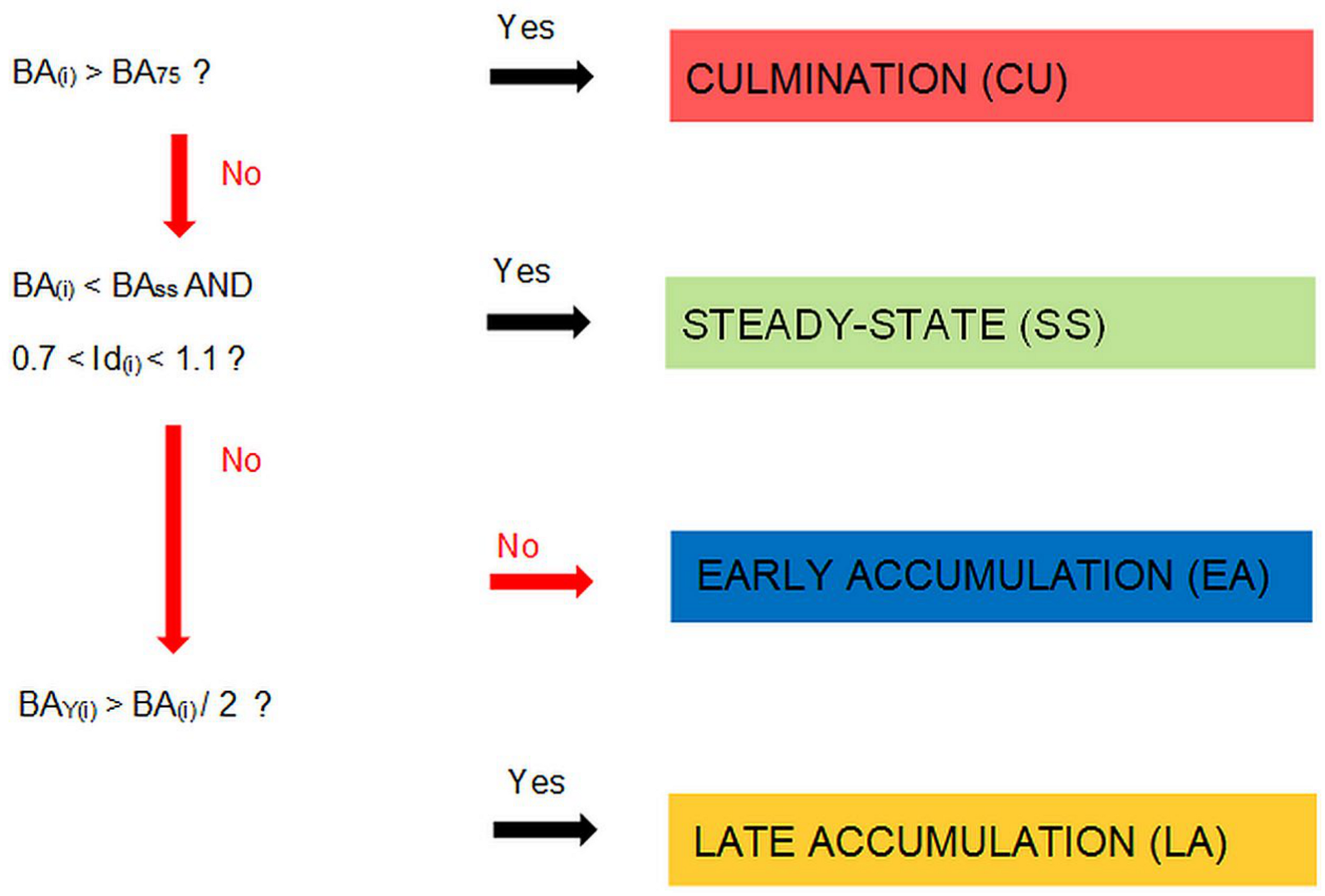
2.1. Patch Classification

The term “patch” used through this paper is defined as an integral forest fragment with explicitly determined boundaries, which represents a given type of forest structure (phase). The boundaries of the stand patches were delineated using the moving window technique, or, in the part of this study based on empirical data, were explicitly linked with the sample plots. The basic structural criteria used for the patch classification were (1) the local biomass accumulation (herein expressed as the local basal area), (2) the differentiation of tree diameters at breast height (dbh), and (3) the proportion of the local basal area fallen relative to trees of young and mature tree generations. These generations were distinguished based on the stand-level median basal area tree diameter, i.e., the dbh, which divides the cumulative basal areas of trees ordered according to ascending or descending dbh into two equal parts. The trees with dbh values lesser or greater than this reference dbh were regarded as young or mature generations, respectively.
Structural differentiation in the stand patches was expressed as the ratio of the empirical dbh variance to a hypothetical variance of the uniform dbh distribution with a predefined lower and upper bound [39]. To put more emphasis on the dbh differentiation among subcanopy trees, which strongly contributes to vertical stand heterogeneity, instead of the dbh, the natural logarithm of this characteristic was used. The ratio, hereafter termed the index of dbh differentiation (Id), was calculated as
I d = S E 2 S U 2 ,
where S2E is the empirical variance of the logarithm of the tree dbh and S2U = (ln dbhmax− ln dbhmin)2/12 is the theoretical variance of the uniform dbh distribution bounded by the minimal and maximal values dbhmin and dbhmax, respectively. The values 7 and 60 cm were assumed as the lower and upper bounds, and in the calculation of the Id index empirical variance S2E, the dbh values of all the trees larger than dbhmax were replaced by the value of 60 cm. This transformation was motivated by the need to construct a dbh-based measure that more strongly corresponds to the vertical structural differentiation than to the absolute dbh variation. Depending on the species and site, in the study region, trees with a dbh of approximately 60 cm attain an average height of 32–35 m. This seems to be a sufficient qualification by which to regard them as individuals from the overstory, considering the average heights for maximal tree dbh classes as being in the range between 42 and 47 m. Thus, the cooccurrence of trees with dbh ≥ 60 cm with other under- and midstory individuals provides a satisfying condition for the assignment of such a forest patch to a multistory, plenter-like type of forest structure. In general, the Id index attains low values for tree collectives with low dbh differentiation, which are values considerably greater than 1 for bimodal dbh distributions, and intermediate values for tree collectives with high dbh differentiation, and the overrepresentation of small trees compared to the uniform distribution. For dbh distributions defined by a geometric sequence
n i = n 1 q i 1 ,
where ni denotes the stem density in the ith dbh class. In the formula, q is the common ratio, q coefficient values are between 0.7 and 0.9 (for a dbh class width of 4 cm), and basal areas are between 35 and 40 m2 ha−1, which are a set of values typical for balanced plenter-like structures and single-tree selection forests in Central Europe, the Id values are in the range between 0.7 and 1.1.
The classification protocol used in this study distinguishes four types of stand structures (phases): culmination (CU), early accumulation (EA), late accumulation (LA), and steady-state phase (SS) (Figure 1). The patches with the highest basal areas of live trees (here, within the upper quartile of this characteristics) were grouped into the culmination phase. Thus, this phase groups stand patches with the highest proportion of large diameter trees. The absolute value of the upper quartile is scale-dependent, and prior to patch classification, it was determined from empirical data (case studies in the Carpathians and Dinaric Mts.) or simulations (in simulation studies). In the latter case, the randomization of tree locations in the subsequent simulations causes the effect in which even for a fixed threshold value of the local basal area, the frequency of patch assignment to the culmination phase fluctuates. By analogy to the concept of dbh equilibrium well-known from single-tree selection forests, the criteria for the steady-state phase were (1) dbh differentiation typical of plenter-like structures and (2) a moderate basal area level. Specifically, the steady-state phase was assigned when the basal area of live trees was equal to or lower than the overall stand-level average and the Id index value was between 0.7 and 1.1. Such a definition warrants that for an ecosystem in a state of dynamic equilibrium (which manifests in insignificant fluctuations in the dbh distribution, biomass level, and species composition over time), increasing spatial scale of analysis will result in an increasing proportion of the steady-state phase. The late accumulation or early accumulation phases were represented by patches that fulfilled the criteria of neither the culmination nor steady-state phase and had a majority of trees representing old or young tree generations (i.e., those with dbh greater than or smaller than the stand-level median basal area tree diameter) in the local basal area (Figure 1). It is assumed that all the threshold values used in the classification, i.e., the average and the upper quartile of the basal area of live trees and the median basal area dbh, are determined for an ecosystem in a state of dynamic equilibrium on a sufficiently large area to minimize scale-dependent fluctuations.

2.2. Simulation Study

In the part of this study based on simulations, the same model stand was used. The dbh distribution was obtained as a geometric sequence (de Liocourt’s distribution) with the parameters (minimal dbh = 7 cm, n1 = 95 stems per ha, and q = 0.811 for 4 cm-width dbh classes) fit to yield a stand basal area of 37 m2 ha−1 and stem density of 500 ha−1, i.e., the values approximately corresponding with the empirical parameters found in old-growth stands in the Western Carpathians [35]. In the first step, simulation tests were performed to demonstrate the effect of the size of the filter used in the moving window procedure on the patch classification outcomes. In subsequent simulations (n = 100), the trees representing the model stand were randomly distributed within a plot of 100 m × 100 m, and the marked point patterns obtained (i.e., tree locations labeled with dbh) were subjected to classification into culmination, early accumulation, late accumulation, and steady-state phases, as defined in the classification protocol (Figure 1). In the classification procedure, circular moving windows with diameters of 10, 15, …, 35 m and a moving distance of 1 m were applied. Edge effects were avoided by using toroidal shifts [28]. For each window diameter variant, 95% envelopes for the phase frequencies, mean patch size, and selected summarizing statistics (basal area, stem density, and index of dbh differentiation) were determined. As a result of the strongly skewed patch size distributions with high frequencies of fine patches, the phase-specific mean patch size s j ¯ was calculated as a weighted average
s j ¯ = i = 1 n w i j s i j i = 1 n w i j ,
where the summation was conducted over all identified patches and weights w i j ( w i j = 1 ) to represent the proportion of the stand area occupied by the ith patch of the jth type (phase) and an area s i j .
In the second step, the original raster models of patch classification (100 × 100 cells) were subjected to noise smoothing by using a majority filter with kernels of 3 × 3, 5 × 5, or 7 × 7 cells. Before replacement in the filtered pattern can occur, the majority filter must satisfy two criteria: (1) the number of neighboring cells of the same value must be the majority of all the cells within a kernel of defined size, and (2) those cells must be contiguous about the center of the filter kernel to minimize the corruption of the cellular spatial patterns. In the simulations (n = 100), for each single cell (1 × 1 m), the structural type (phase) was assigned based on the tree collectives located within the window section, and then a few runs of the majority filter were conducted until the output raster was stabilized (no further changes occurred), and a smoothed pattern was obtained. Then, 95% simulation envelopes for the phase frequencies, mean patch size, and selected summarizing statistics (dbh distribution, basal area, stem density, and index of dbh differentiation) were determined for the individual phases and compared between the original and filtered (smoothed) patterns.
The third simulation experiment was programmed to illustrate that the moving windows with overlap applied for random spatial patterns of tree distribution artificially generated spatial dependence of phase distributions (patchiness). The intensity of the overlap was defined as the ratio of the window diameter to the moving distance. Under this formulation, the neighboring moving windows did not contain common trees for the ratio equal to 1, and the proportion of shared trees increased for the ratio values greater than 1. In the subsequent simulations (n = 100), random tree distributions of the model stand were generated on a 100 m × 100 m plot (10,000 cells). Then, the patch classification (window size = 15 m) and, as additional variants, smoothing procedures with the kernel sizes of 3 × 3, 5 × 5, or 7 × 7 cells were performed. Within the plot, the cells were selected in a square lattice to produce window diameter: moving distance ratios between 0.5 and 4.0, and the classification outputs for these cells were recorded. Finally, for each overlap ratio and smoothing variant, the proportion of positive indications of spatial dependence (i.e., significant departures from the null hypothesis assuming random labeling of the sample plots with phase qualifiers) was compared. As a measure of spatial dependence, the mark connection function was used [40], which, here, determines the probability that a randomly selected pair of sample plots located at most r distance units apart represent the same phase:
p r = N r 1 i = 1 N r n r .
In the formula Nr denotes the number of all distinct pairs located at most r distance units apart, maximal r is 50 m, and nr equals 1 when the sample plots belong to the same phase and 0 otherwise. A Monte Carlo procedure based on 10,000 simulations was applied to test the significance of the departures from the null hypothesis, assuming random labeling. The overall intensity of the positive spatial dependence was expressed as the average positive deviation
k r 1 p r E r U r E r 1 ,
where the summation is applied over kr, the number of all distance units r so that p(r) > Ur, Ur is the upper simulation envelope, and Er is the mean value of p(r) for random labeling. All the computations were programmed by the author in the Visual Basic for Applications programming language (VBA).

2.3. Randomness vs. Patchiness—Empirical Examples

The empirical data used herein originated from six strict reserves located in the Dinaric Mountains (Janj, Lom, and Perućica) and Western Carpathians (Baniska, Oszast, and Żarnówka) (Table 1). The strict reserves selected for this study are relic, old-growth forests of the lower montane belt in Europe formed by silver fir Abies alba Mill., European beech Fagus sylvatica L., and Norway spruce Picea abies (L.) H. Karst with no documented history of past forest management. The term “old-growth forests” is used here to underscore that the core zones of the reserves bear no signs of direct human activity (stumps, cut trees, logging trails, under-planting, simplified vertical stand structure). Nevertheless, plunder-like cuttings of single trees may have occurred in the past. The Janj, Lom, and Perućica reserves have been officially strictly protected since the 1950s, but there is also evidence that strict nature protection in these areas goes back to the 19th century during the Austro-Hungarian Empire [41]. Although the periods of formal strict protection differ in the Baniska, Oszast, and Żarnówka reserves (Table 1), this factor cannot be treated as a measure of the human impact on stand dynamics. In all the reserves, the primary reason for protection was the high level of preservation of natural stands, which was probably stemming from terrain inaccessibility, past patterns of extensive forest land utilization, and the economic infeasibility of logging. The study stands certainly belong to the best maintained mixed-species forests in the Dinaric Mts. and Western Carpathians [42].
The Dinaric Mountains harbor one of the most volume-rich mountain primeval forests on the continent, with growing stocks commonly exceeding 1000 m3 per ha. In contrast, in the Western Carpathians, which are the northernmost region of occurrence of such forests, average stand volumes are only half of those reported in the Balkans, which probably is attributable to a more a severe disturbance regime in this region [43]. Thus, the study sites selected for this research characterize a possibly wide range of climatic conditions and disturbance regimes in which the remnants of the former pristine fir–beech–spruce forests still can be found. Data on the location, site conditions, and protection history are summarized in Table 1.
In each of the reserves, one close-to-rectangular research area of approximately 10 ha in size with a minimal length of the narrower side of 160 m was established. The fragments selected for the survey were as homogeneous as possible in terms of site conditions, species composition, and terrain orography and showed no signs of direct human activity. In each research area, between 237 and 259 circular sample plots with a radius of 7 m were localized in a regular lattice of 20 m × 20 m. The dbh and species of all live trees with dbh ≥ 7 cm were registered on the sample plots. In this spatial scale, the mean stem densities were between 4.4 and 10.4 and the 10th percentiles were between 2 and 5 trees, which provided a sufficient basis for the classification of the structural types (phases). On the other hand, the diameter of the sample plots (14.0 m) was considerably larger than the nearest-neighbor distances among trees classified into the old generation (i.e., with dbh greater than the stand-specific median basal area tree diameter) assuming their random distribution (7.5−9.2 m), and close to the nearest-neighbor distance for a hexagonal distribution, i.e., the maximal packing of such trees (14.4−17.6 m). Considering that the crown radii of average canopy trees are less than the radius of the sampling plots, even for very regular distribution patterns, the sampling design warranted the identification of hot spots for generation replacement—that is, stand fragments without trees representing the old generation. Table 2 contains the basic stand characteristics and stand-specific reference values used in the patch classification (Figure 1)—that is, BA75, BAss, and dbhBA. Insignificant variation of the reference values within the geographic regions (i.e., Dinaric Mts and Western Carpathians) suggests that they provide reliable estimates for hypothetical steady-state conditions. The dbh distributions and selected characteristics of spatial tree distributions in the studied stands (e.g., the randomness and independence of the distribution across tree size categories and the spatial variation of the basal area and dbh differentiation) were published formerly [35,43,44].
The underlying null hypothesis of random patterns of structural heterogeneity was divided into two hierarchical components: (1) the random assignment of tree dbh to the sample plots and (2) the spatial independence of the distribution of the sample plots representing given structural types (phases). In the first case, the original tree counts on the sample plots were maintained, the trees were randomly assigned to the sample plots, and the sample plots were classified according to the rules defined above. Based on subsequent simulations (n = 10,000), 95% envelopes for the phase frequencies were constructed and compared with the classification outputs based on the empirical sets. Thus, the empirical values lying above/below the simulation envelopes indicate the over/underrepresentation of a given phase compared to the frequency expected for the random assignment.
In the case of testing the spatial independence of the phase distribution, in the simulations, the sample plots were randomly labeled with phase qualifiers (n = 10,000 simulations), and 95% envelopes for the statistics based on the mark connection function p(r) defined above were constructed and compared with the empirical data. In this case, empirical values greater than the upper simulation envelopes indicated a positive spatial correlation (aggregation = patchiness), and values lower than the lower envelopes indicated a negative spatial correlation of the phase distribution (segregation = intermingling stronger than expected from random labeling). The tests were performed for all the phases pooled together (null hypothesis: spatial independence of the phase distribution) and separately for each phase (null hypothesis: spatial independence of the distribution of a given phase). In this latter case, the subsequent tests were not independent (e.g., the aggregation of one phase involves the apparent aggregation of the other). To avoid this linkage, a stepwise procedure was applied. First, the phase showing the largest significant departure from the random labeling hypothesis was found. In subsequent simulations, the labeling of the sample plots representing this phase was preserved but carried out randomly for other plots.

3. Results

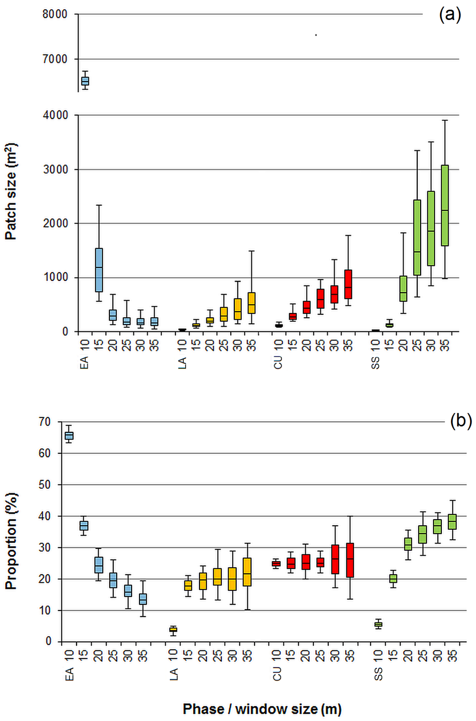
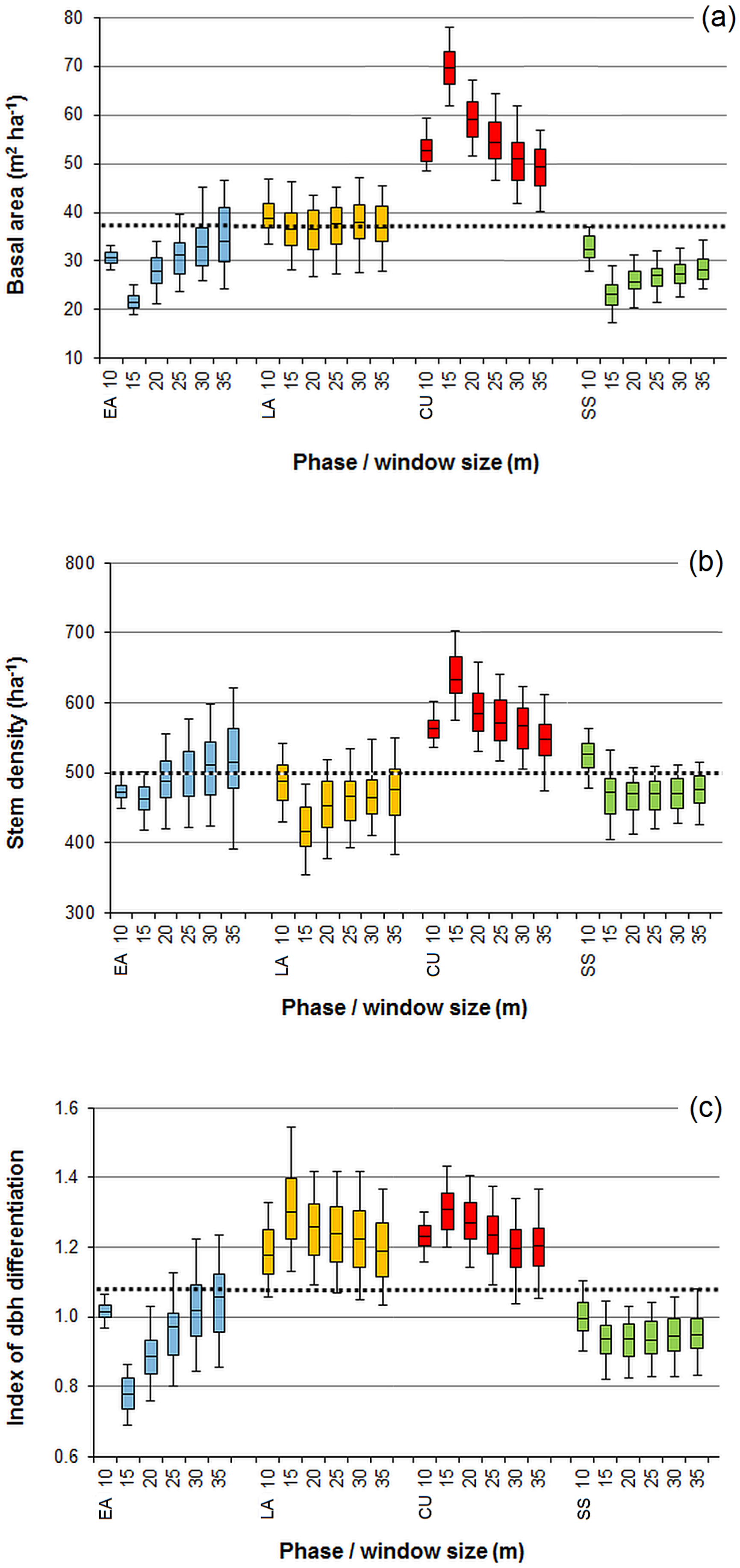
3.1. Effect of the Moving Window Size

Applying the technique of the moving windows with overlap (i.e., the moving distance is smaller than the window diameter) for the classification of tree collectives assembled by chance (based on random tree distributions) produced patch-mosaic patterns with clear aggregation of the classification outputs. The moving window diameter had a substantial effect on the patch-mosaic pattern (Figure 2). A general trend was that with increasing window sizes, the patterns changed from fine- to coarse-grained. This tendency emerged for all the phases except for the early accumulation phase in which the average patch area decreased with increasing window diameters (Figure 2 and Figure 3). When the window size was ≤15 m, the largest patches formed the early accumulation phase, but for larger filter sizes, the aggregations of the steady-state phase dominated. Increasing window diameters strongly increased the absolute variation of the average patch area for the steady-state phase and decreased it for the early accumulation phase (Figure 3).
The spatial scale of the neighborhood considered in the classification procedure also strongly influenced the proportions of the area assigned to the structural types (Figure 3). This effect was particularly noticeable in the case of the early accumulation and steady-state phases and less evident in the late accumulation phase. The frequency of the culmination phase remained insensitive, because the fixed value of the local basal area was predefined as a minimal threshold in the classification protocol. The dominant tendency was that the early accumulation phase strongly diminishes and the steady-state phase increases its proportion with the increase in the window diameter. Increasing window diameters tended to increase the absolute variation in the frequencies of the culmination and late accumulation phases but not of the early accumulation and steady-state phases (Figure 3).
The window diameter affected also the variation in the basal area, stem density, and dbh differentiation between the phases (Figure 4). Except for the smallest filter (10 m), the general tendency was that the between-phase variation diminished with increasing window diameters. Particularly scale-sensitive were the basal area of the culmination and early accumulation phases and the dbh differentiation of the early accumulation phase. The diverging behavior of the summarizing characteristics for the smallest window diameter (10 m) was attributable to differences in variable distributions, which, in opposition to the bell-shaped forms found for larger filters, in this case, was truncated at low values of the variables.

3.2. Effect of Noise Smoothing

Figure 5 portrays the effects of noise smoothing by using a majority filter algorithm with kernels of 3 × 3, 5 × 5, and 7 × 7 cells (filtered patterns). The smoothing procedure considerably changed the classification outputs of the single cells. The simulations showed that the proportion of altered cell values ranged between 20% and 60% and tended to increase with increasing kernel sizes (Figure 6). The proportion of changes is important, as it may be viewed as a bias introduced by the smoothing procedure.
The pattern attributes derived from the original and filtered patterns differed in terms of both the phase frequency and the average patch size of the individual phases (Figure 7). With increasing kernel sizes, the filtered patterns became more coarse-grained, and the average patch size increased for all the phases. The noise-smoothing procedure also increased the representation of the phases that were more frequent in the original pattern. The phase-specific dbh distributions constructed for the filtered patterns were characterized by a higher variation of tree counts in the dbh classes compared to those derived from the original patterns, particularly in the case of the phases of low frequency (Figure 8).

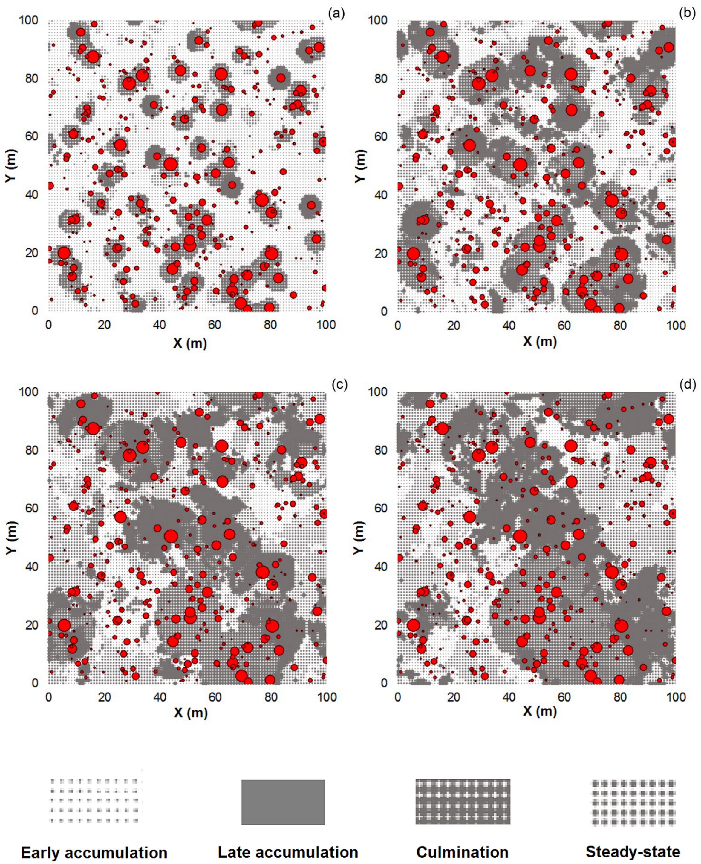
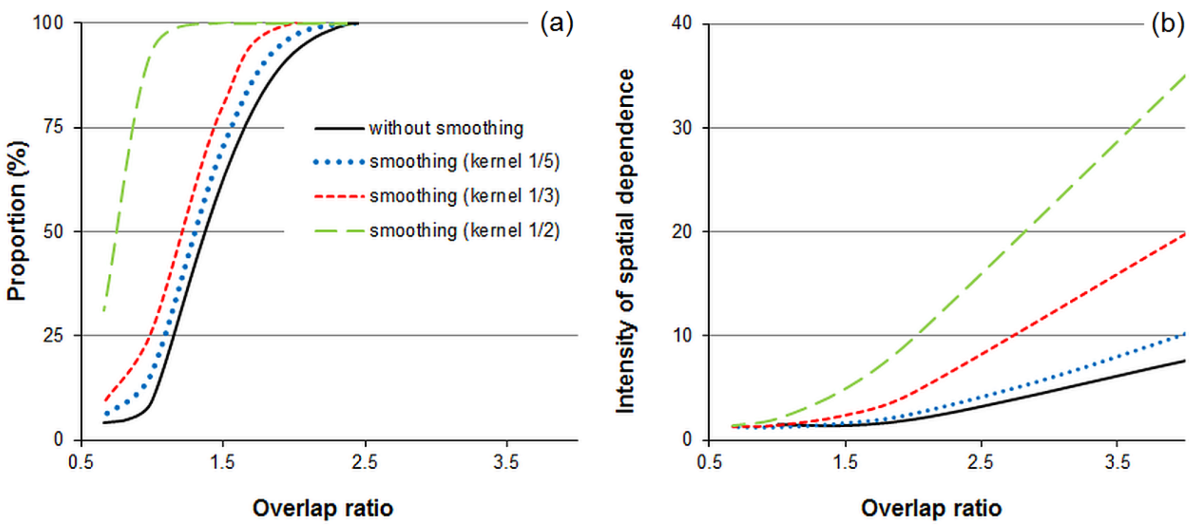
3.3. Effect of Overlapping Windows on the Spatial Dependence of the Phase Classification Outputs

The tests indicated that the technique of moving windows with overlap artificially produces spatial dependence between classification outputs, even for random tree distributions (Figure 9). For the original raster models of phase classification, the proportions of positive identifications of spatial dependence were 93 and 100% for the overlap ratios of 2.0 and 4.0, respectively. Moreover, noise smoothing using the majority filter additionally intensified the spatial dependence between the neighboring stand patches, and this effect was stronger with larger kernel filter sizes. Noise smoothing evoked spatial correlations, even for spatially independent tree collectives—that is, for nonoverlapping windows. For the overlap ratio of 1 and kernels between 1/5 and 1/2 of the window size, the proportion of positive identifications of spatial correlation was between 16 and 31% (Figure 9). Thus, these results indicate that the spatial correlation found in the phase distribution patterns generated by the procedure of moving windows with overlap should not be directly interpreted as evidence of spatial correlation in the original tree distribution pattern, which, in the simulations used here, was completely random. For unbiased inference, the samples should be spatially independent, or the spatial dependence inherently produced by the spatial overlap of the moving windows should be considered in the testing procedure.

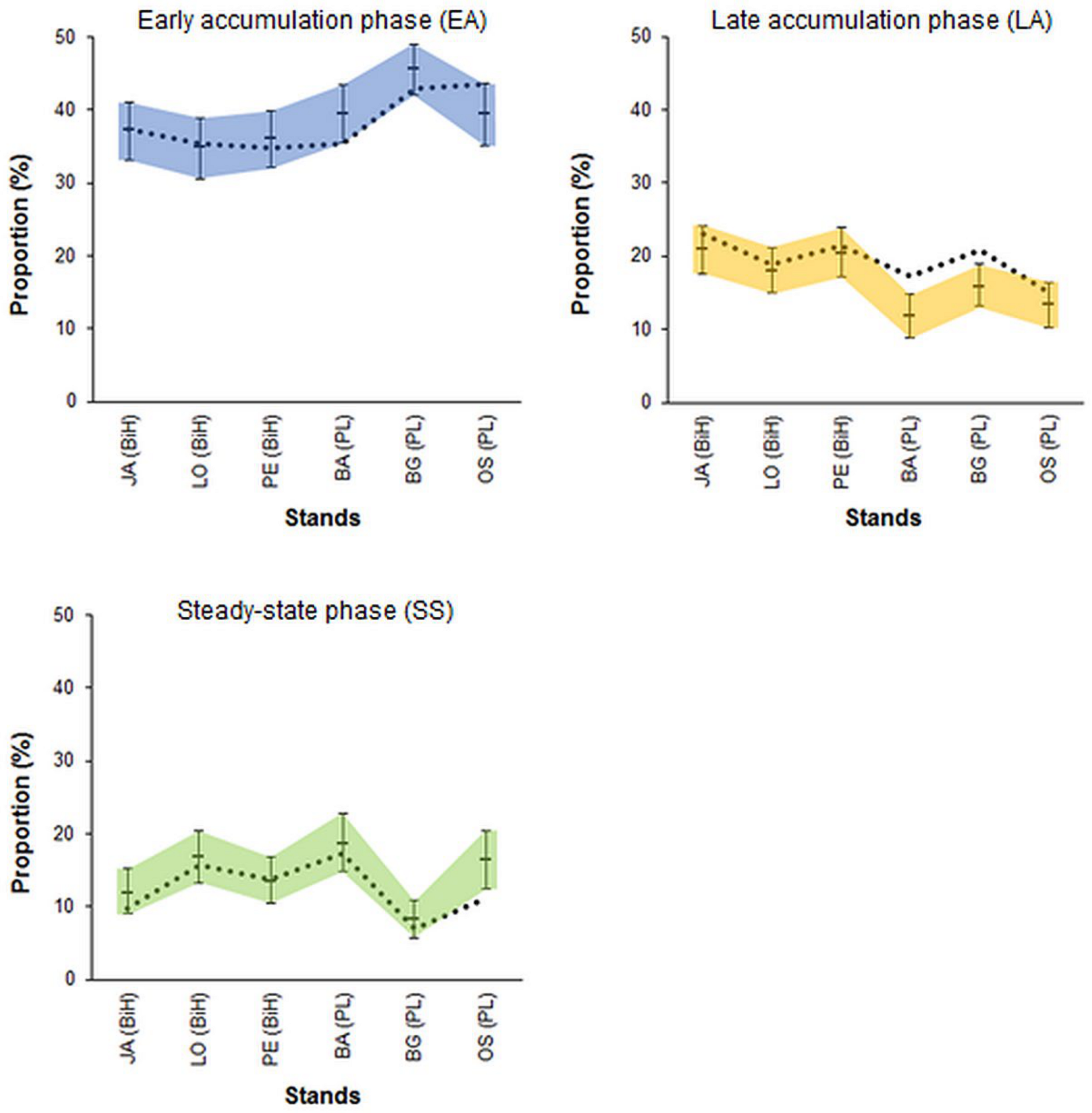
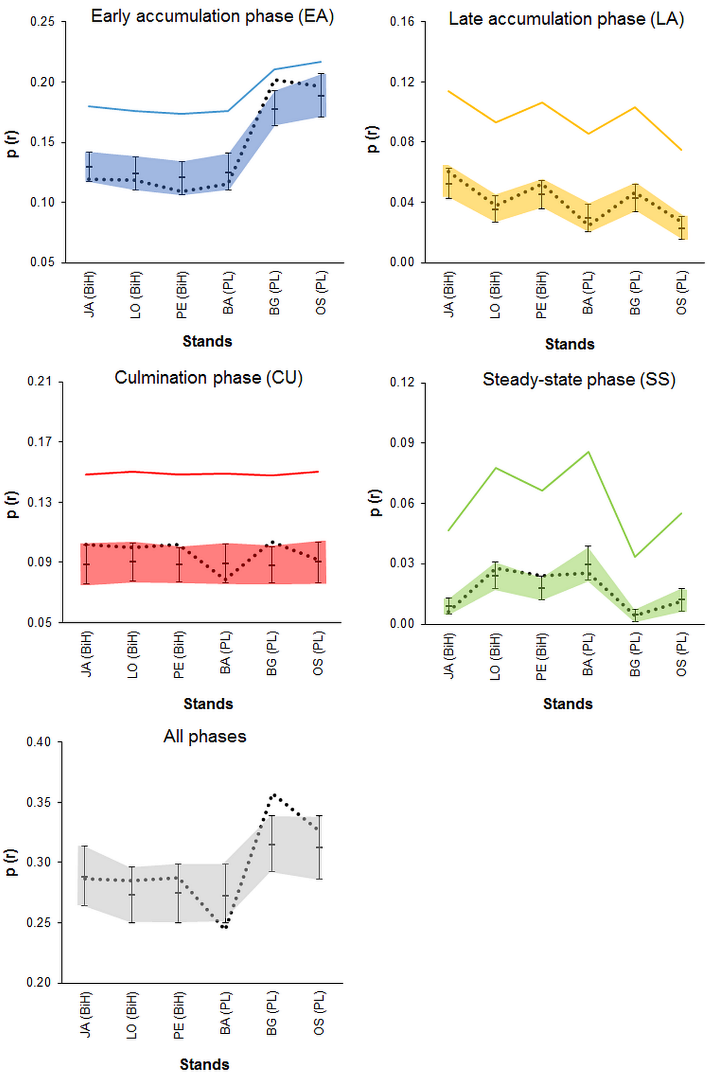
3.4. Randomness vs. Patchiness-Empirical Examples

For testing the spatial dependence in real stands, the datasets from six old-growth Abies–Fagus–Picea forests from the Dinaric Mountains (JA, LO, PE) and Western Carpathians (BA, BG, OS) were used (Table 1 and Table 2). Figure 10 displays the empirical phase frequencies on the backgrounds of the simulation envelopes for the expected frequencies resulting from the random assignment of tree dbh to the sample plots. Except for several cases, the empirical frequencies did not deviate from the values obtained in the simulations. The analyses indicated that the early accumulation phase was significantly underrepresented in one stand (BA; in BG, the null hypothesis was close to rejection) and overrepresented in one stand (OS). The steady-state phase was underrepresented in one stand (OS), and the late accumulation phase was overrepresented in two stands (BA and BG) (Figure 10). Nonetheless, compared to the expected frequencies, represented here by the simulation envelops, the deviations were minor.
The null hypothesis of an independent phase distribution (all phases pooled together) could be rejected in two stands at the scale of 800 m2 (BG and OS) and two stands at the scale of 1600 m2 (BA and BG). However, the deviations were weak, and in the latter case, they were both positive (BG stand) and negative correlations (BA stand) (Table 3). A deepened analysis revealed that in the OS stand, the deviations toward aggregation were mainly attributable to the positive spatial dependence of the early accumulation phase and, in the BG stand, they were mainly attributable to the culmination phase (Figure 11). Significant aggregation was also revealed for the culmination phase in the JA stand and for the culmination and steady-state phases in the PE stand, but these effects were too weak to generate a positive spatial correlation for all the phases pooled together. Compared to a pattern that fulfills the majority criterium used by the smoothing procedure (i.e., half of the neighboring plots represent the same phase as the central plot), in the empirical patterns, the spatial aggregation of the phases was very weak (Figure 11).

4. Discussion

4.1. Remarks on the Phase Classification Protocol

In the literature, several methods of phase classification dedicated to multiaged forests have been proposed. In the classical founding works [15,16,45,46,47], the classification criteria were verbally expressed and associated with anticipated changes in the stand growing stock, canopy closure, vertical stand structure, proportion of individuals representing distinct age cohorts, or the necromass of dead trees. More recently, methods based on quantitative criteria have been developed, which help make the distinction objective and repeatable [17,18,19,22,48]. Nevertheless, different classification systems can lead to largely deviating results [26,48]. In addition, some of these propositions are based on scale-sensitive standards (e.g., the presence/absence of trees from given dbh classes), and the classification outputs strongly depend on the spatial scale being considered [19,22]. Feldmann et al. [26] proposed a scale-independent approach based on the relative frequencies of trees representing three ontogenetic stages [49]. However, it seems that this method circumvented the problem by eliminating from the classification the type of multisized stand structures (here, represented by the steady-state phase), whose proportion usually increases at the expense of other phases along with increasing the spatial scale of the analysis. In this study, the local basal area, the proportion of trees with dbh above the given dbh threshold (median basal area dbh), and the dbh differentiation expressed by the Id index were used as classification criteria. Unlike other propositions, the structural differentiation was considered explicitly only for the steady-state phase. In addition, the upper boundary for growing stock in this phase was defined to underline the dynamic attributes of this type of structure and its link with the balanced dbh structures known from managed forests under single-tree selection systems. Herein, the threshold value was set arbitrarily as the mean stand basal area, with the consequence that increasing the spatial scale results in increasing the proportion of the steady-state phase, concordantly with J-shaped dbh distributions and the all-aged character of the study stands. This threshold value may be easily adapted to local conditions, depending on the site, species composition, and local knowledge of the dynamics of structured forests [50,51,52]. Nonetheless, neglecting this factor and using only structural diversification as the sole criterion for the steady-state phase may lead to its overrepresentation and discrepancies with the results of classical studies indicating relatively small proportions of this planter-like phase in primeval forests containing European beech, Norway spruce, and silver fir [45,53].
The culmination phase groups stand patches with the highest basal area and therefore is similar to the optimum phase defined in earlier studies [15,16,47]. Nonetheless, in opposition to these classical works, the culmination phase was not linked with a low level of structural differentiation. The sole criterion here was a high level of basal area associated with local overrepresentation of the overstory trees. This seems justified by the results of studies showing that in European natural montane forests formed by shade-tolerant species, multisized structures are dominant, even at small spatial scales [34,35,36,37,38,54,55,56,57], and that stand biomass accumulation at the local scale does not entail simplification of the forest structure. Indeed, the small-scale analyses conducted in the six stands used in this study revealed that even for the highest levels of growing stocks, the stem numbers were evenly distributed among the dbh classes [58].
The classification protocol used in this study passed over dead trees, which are usually regarded as imprints of the past stand dynamics and are frequently included in phase classification systems [16,19,22,48]. However, Král et al. [59] found a dominant role of acyclic transitions between “structural” phases in the natural forests of the temperate zone, which weakens the indicative value of dead trees. In addition, the relationships between the necromass of dead trees and the growing stock of living trees are usually weak [9]. In the stands studied here, the Pearson’s correlation coefficients between these characteristics were in the range between −0.10 and −0.25 [58], no matter whether single plots (with a diameter of 14 m) or larger blocks of neighboring plots were considered. These weak relationships are attributable to the fact that coarse woody debris—especially those from conifer species—are recognizable over several decennia [25,60,61,62,63,64], that is, at the temporal scales upon which substantial changes among live trees usually occur [65,66,67]. On the other hand, recent disturbances resulting in the presence of fresh deadwood also affect the structural attributes of living tree collectives. Thus, information on dead trees seems excessive, and in some situations in which the time since tree death is difficult to determine, it may burden the reconstruction of the local development pathway.

4.2. Limitations of Using Moving Windows with Overlap for Patch Classification

The simulation study clearly demonstrates that in multiaged forests with reversed J-shaped dbh distributions, the frequencies, patch sizes, and variation in phase-specific structural attributes (e.g., basal area, stem density, dbh distributions, etc.) strongly depend on the window size and kernel used in the smoothing procedure and that results obtained using different settings of these parameters should not be compared. The results resemble former findings indicating that phase classification outputs depend on the spatial scale being considered [23,68,69] and that rapidly increasing proportions and average patch sizes of the stand fragments with complex dbh structures close to the overall stand-level distribution are a universal feature of multiaged forests with strongly randomized patterns of structural heterogeneity [18,35,43,56,70,71,72].
Areas between 100 and 500 m2 are commonly treated as the basic spatial units in analyses of structural heterogeneity [17,18,19,48,73,74]. The present study shows that increasing window sizes results in more and more smooth patterns of structural heterogeneity, decreases between-patch variation, and leads to losses of information on the local configurations of trees and the patterns of tree generation replacement (single-tree vs. group replacement). On the other hand, areas that are too small involve a risk of overlooking overstory trees growing in the close neighborhood and thus impeding the ingrowth of understory individuals and misinterpreting such fragments as hotspots of generation replacement. From this point of view, a plausible recommendation is to keep the basic window diameter (or plots used for sampling) close to the average area occupied by overstory individuals, assuming their more-or-less regular distribution, as frequently reported by studies of natural forests [31,35,43]. Regarding trees with dbh over the median basal area dbh as a mature generation, the maximal nearest-neighbor distances for their hexagonal distribution in the studied stands were within a relatively narrow range between 14 and 18 m. Under real conditions, such a regular distribution of the canopy trees is unlikely, and the nearest-neighbor distances will certainly be smaller. This range gives an average area per individual of approximately 150−250 m2, which corresponds well with the gap area distributions found in close-to-primeval montane forests formed by shade-tolerant species in Europe, indicating the dominance of small gaps caused by the deaths of single trees or small groups of trees [10,17,75,76,77,78,79,80]. Nevertheless, depending on the objective of the analysis (the types of forest structure, growing stock of living or dead trees, stem density, etc.) the optimal plot sizes differ [81,82,83,84].
The original pattern of cell classification (without smoothing) most fully reflects the frequency and phase-specific characteristics. In particular, it provides estimates concordant with these derived from sampling using inventory plots of the same size as the moving window. The smoothing procedure based on the majority filter distorts the original pattern, generally diminishes the proportions of phases underrepresented in the original image, and causes the estimates obtained from hypothetical inventory plots to not converge to those derived from the smoothed pattern. The simulations showed that this biasedness, even for 3 × 3 kernels producing relatively fine-grained patterns with a considerable proportion of very small patches, is between 20 and 30% and strongly increases with the kernel size to an unacceptable level. Thus, patch classification outputs obtained from sampling based on inventory plots (including the rather extreme case of absolute contiguous plots) and moving window procedures with noise smoothing, as a rule, are different, and the level of biasedness may easily exceed the phase frequencies.
The main problem associated with using patterns transformed by the moving window technique is that this procedure inherently produces positive spatial correlations, as overlapping windows, depending on the moving distance and window size, share the same trees. Therefore, such transformed patterns are characterized by patchiness sensu stricto, even for completely random tree distributions. As evidenced by the simulation experiment, the completely randomized patterns transformed by using sliding windows overlapping by one-half of their diameters were falsely classified as patchy in approximately 93% of the cases, and after smoothing, this proportion was 100%. Moreover, the noise smoothing imposed spatial correlations even for independent tree collectives from nonoverlapping windows. Therefore, the technique of moving windows with overlap is helpful for visualizing spatial structural heterogeneity but inappropriate for testing whether this variation is random. For this purpose, spatially independent samples must be used (for example, contiguous windows), or the spatial correlation unavoidably generated by the overlapped samples should be taken into account in the testing procedure. Grabarnik et al. [85] also stressed the importance of considering the spatial dependence in hierarchical multiscale tests in which a range of distances is simultaneously being tested. More recently, an interesting method of patch delineation was proposed [79]. In this method, instead of setting an arbitrary fixed window diameter, the scale was allowed to “float” as a function of the actual spatial positioning of trees, and neighborhood patches were identified through spatial tessellation. Nevertheless, because each tree was a component of several other neighborhoods and the patches overlapped, this approach also seemed to suffer from the spatial dependence problem.

4.3. Randomness vs. Patchiness-Empirical Examples

The analyses based on empirical data indicated that in a majority of the cases, the null hypothesis assuming the random assignment of tree sizes to the sample plots could not be rejected. Similar results provided tests of the spatial independence of the phase distribution. Moreover, in all the empirical stands, the aggregation of the phases was much weaker than in a hypothetical pattern in which the majority of the nearest-neighboring four to eight plots represent the same structural type as the center plot. Although the tree distribution patterns were analyzed here at a discontinuous spatial scale (plots at 154 m2 and their neighborhood at 400 and 800 m2), it seems unlikely that this factor could significantly influence the results, since, as shown in the simulations, within the range of spatial scales considered in this analysis, the changes in structural attributes follow a gradual and not erratic manner. The obtained results indicate on the dominance of random components in forming structural heterogeneity and thus contradict the presumption that patchiness sensu stricto is a common and general feature of the studied forest communities.
This conclusion well corresponds with research suggesting that structural heterogeneity occurs primarily in small areas and diminishes rapidly with increasing spatial scales [70,71,81]. Although homogeneously structured patches occur, they cover a smaller proportion of the total forest area than those that are heterogeneously structured [34,35,43,54,55,56,57,86]. Glatthorn et al. [87] concluded that forest development takes place on a continuous scale and that discrimination between development stages splits continuous datasets at selected thresholds. Recently, Zenner et al. [71] proposed a gap-patch reabsorption model that assumes that gaps continuously and stochastically created through individual tree mortality and even intermediate-intensity disturbances are quickly reabsorbed back into the general fabric of the highly heterogeneous background forest matrix in which they are embedded. Therefore, patchiness is predominantly a fine-scale phenomenon, and individual patches are often transient.
The concept of patchiness sensu stricto implies that the stand patches maintain their spatial integrity over time and evolve in a cyclic sequence dependent on the maturing and senescence of trees forming the overstory. However, Christensen et al. [88] and Král et al. [59] showed that over the long term, frequent partial disturbances followed by quick recovery results in highly stochastic connections between different multiaged phases, and the proportion of cyclic transitions is significantly less frequent than that of acyclic transitions along theoretical pathways. Thus, these results also indicate the prevalent role of random mortality among the overstory trees and contradict the concept of patchiness sensu stricto.
The dominance of random components in forming structural heterogeneity does not exclude that some processes generate nonrandom effects. Repulsion or attraction among trees representing different species or size classes is commonly reported by studies concerned with the structural heterogeneity of forest communities and attributed to intraspecific competition [89,90], interspecific facilitation [91,92], environmental heterogeneity [93], dispersal limitations [94], or factors responsible for tree mortality phenomena [95]. The methodology based on the classification of tree collectives also has the potential to provide information concerning spatial relationships between tree subpopulations and underlying ecological processes. It operates on a higher level of structural organization of forest communities and therefore may help solve problems for which statistical models based on spatial point processes become complicated [96]. Nonetheless, passing from description to interpretation necessitates a fundamental distinction between random and nonrandom patterns.

5. Conclusions

This paper aimed to emphasize the distinction between spatial structural heterogeneity (patchiness sensu lato) and patchiness sensu stricto viewed as the spatial ordering of tree attributes differently from a random pattern. While the first is a common feature of all forest stands except those formed by equisized and regularly distributed individuals, the second has functional interpretation and is attributable to working ecological processes that spatially organize the structural heterogeneity of forest communities.
This study showed that the outcome patterns produced by the sliding window with overlap are characterized by inherent spatial correlations and are falsely interpreted as patch mosaics, even for originally completely random tree distributions. Thus, this technique is a useful tool for portraying the spatial structural heterogeneity of forest stands but inappropriate for the assessment of the random or nonrandom character of the observed pattern. In the latter case, the samples must fulfill the criterion of spatial independence, and the windows used for classification of the tree collectives should not overlap. The moving window size strongly affects the patch frequency, mean patch size, and between-patch dbh differentiation, and therefore, the choice of this parameter should consider the aim of the analysis. For studies focusing on the pattern of generation replacement, a starting point would be the window size corresponding to an average area of a single overstory tree.
The analyses carried out in six stands from the Dinaric Mountains and Western Carpathians using a methodology based on spatially independent samples indicated that patchiness sensu stricto is not a general feature of the forest communities formed by silver fir, European beech, and Norway spruce. The study shows that in addition to random patterns of structural heterogeneity, spatial segregation and aggregation of structural types can also occur. A further study is warranted concerning the issue of whether the general pattern of structural heterogeneity changes over time and which processes are behind such possible shifts.

Funding

The data collection was supported by the scholarship funds from the University of Agriculture in Krakow (Poland) for JP. The publishing was financed by a subvention from the Ministry of Science and Higher Education of the Republic of Poland for the University of Agriculture in Krakow for 2020 (SUB/040012/D019).

Institutional Review Board Statement

Not applicable.

Informed Consent Statement

Not applicable.

Data Availability Statement

The datasets used and/or analysed during the current study are available from the corresponding author on reasonable request.

Acknowledgments

The author wishes to thank Z. Govedar (University in Banja Luka, Bosnia and Herzegovina) and S. Keren, for their help in organizing his stay in the Dinaric Mountains.

Conflicts of Interest

The author declares that he has no competing interest.

References

  1. Brown, C.; Law, R.; Illian, J.B.; Burslem, D.F.R.P. Linking ecological processes with spatial and non-spatial patterns in plant communities. J. Ecol. 2011, 99, 1402–1414. [Google Scholar] [CrossRef]
  2. Illian, J.B.; Burslem, D.F.R.P. Improving the usability of spatial point process methodology: An interdisciplinary dialogue between statistics and ecology. AStA Adv. Stat. Anal. 2017, 101, 495–520. [Google Scholar] [CrossRef] [Green Version]
  3. Velázquez, E.; Martínez, I.; Getzin, S.; Moloney, K.A.; Wiegand, T. An evaluation of the state of spatial point pattern analysis in ecology. Ecography 2016, 39, 1042–1055. [Google Scholar] [CrossRef]
  4. Law, R.; Illian, J.B.; Burslem, D.F.R.P.; Gratzer, G.; Gunatilleke, C.V.S.; Gunatilleke, I.A.U.N. Ecological information from spatial patterns of plants: Insights from point process theory. J. Ecol. 2009, 97, 616–628. [Google Scholar] [CrossRef]
  5. Watt, A.S. Pattern and process in the plant community. J. Ecol. 1947, 35, 1–22. [Google Scholar] [CrossRef] [Green Version]
  6. Remmert, H. The Mosaic-Cycle Concept of Ecosystems; Remmert, H., Ed.; Springer Verlag: New York, NY, USA, 1991; pp. 1–21. [Google Scholar]
  7. Firm, D.; Nagel, T.A.; Diaci, J. Disturbance history and dynamics of an old-growth mixed species mountain forest in the Slovenian Alps. For. Ecol. Manag. 2009, 257, 1893–1901. [Google Scholar] [CrossRef]
  8. Hobi, M.L.; Commarmot, B.; Bugmann, H. Pattern and process in the largest primeval beech forest of Europe (Ukrainian Carpathians). J. Veg. Sci. 2015, 26, 323–336. [Google Scholar] [CrossRef]
  9. Feldmann, E.; Drößler, L.; Hauck, M.; Kucbel, S.; Pichler, V.; Leuschner, C. Canopy gap dynamics and tree understory release in a virgin beech forest, Slovakian Carpathians. For. Ecol. Manag. 2018, 415/416, 38–46. [Google Scholar] [CrossRef]
  10. Orman, O.; Dobrowolska, D. Gap dynamics in the Western Carpathian mixed beech old-growth forests affected by spruce bark beetle outbreak. Eur. J. For. Res. 2017, 136, 571–581. [Google Scholar] [CrossRef]
  11. Brang, P.; Spathelf, P.; Larsen, J.B.; Bauhus, J.; Boncina, A.; Chauvin, C.; Drössler, L.; Garcia-Guemes, C.; Heiri, C.; Kerr, G.; et al. Suitability of close-to-nature silviculture for adapting temperate European forests to climate change. Forestry 2014, 87, 492–503. [Google Scholar] [CrossRef] [Green Version]
  12. Petritan, I.C.; Commarmot, B.; Hobi, M.L.; Petritan, A.M.; Bigler, C.H.; Abrudan, I.V.; Rigling, A. Structural patterns of beech and silver fir suggest stability and resilience of the virgin forest Sinca in the Southern Carpathians, Romania. For. Ecol. Manag. 2015, 356, 184–195. [Google Scholar] [CrossRef]
  13. Janík, D.; Král, K.; Adam, D.; Hort, L.; Samonil, P.; Unar, P.; Vrška, T.; McMahon, S. Tree spatial patterns of Fagus sylvatica expansion over 37 years. For. Ecol. Manag. 2016, 375, 134–145. [Google Scholar] [CrossRef] [Green Version]
  14. Seidl, R.; Thom, D.; Kautz, M.; Martin-Benito, D.; Peltoniemi, M.; Vacchiano, G.; Wild, J.; Ascoli, D.; Petr, M.; Honkaniemi, J.; et al. Forest disturbances under climate change. Nat. Clim. Chang. 2017, 7, 395–402. [Google Scholar] [CrossRef] [PubMed] [Green Version]
  15. Leibundgut, H. Europäische Urwälder; Paul Haupt: Bern, Switzerland, 1993. [Google Scholar]
  16. Korpel’, Š. Die Urwälder der Westkarpaten; Gustav Fisher Verlag: Stuttgart, Germany, 1995. [Google Scholar]
  17. Meyer, P. Bestimmung der Waldentwicklungsphasen und der Texturdiversität in Naturwäldern. Allg. Forst u. J. Ztg 1999, 170, 203–211. [Google Scholar]
  18. Emborg, J.; Christensen, M.; Heilmann-Clausen, J. The structural dynamics of Suserup Skov, a near-natural temperate deciduous forest in Denmark. For. Ecol. Manag. 2000, 126, 173–189. [Google Scholar] [CrossRef]
  19. Tabaku, V. Struktur von Buchen-Urwäldern in Albanien im Vergleich mit deutschen Buchen-Naturwaldreservaten und—Wirtschaftswäldern; Cuvillier Verlag: Göttingen, Germany, 2000. [Google Scholar]
  20. Drössler, L.; Meyer, P. Waldentwicklungsphasen in zwei Buchen-Urwaldreservaten in der Slowakei. Forstarchiv 2006, 77, 155–161. [Google Scholar]
  21. Podlaski, R. Dynamics in Central European near-natural Abies-Fagus forests: Does the mosaic-cycle approach provide an appropriate model? J. Veg. Sci. 2008, 19, 173–182. [Google Scholar] [CrossRef]
  22. Král, K.; Vrška, T.; Hort, L.; Adam, D.; Šamonil, P. Development phase in a temperate natural spruce-fir-beech forest: Determination by a supervised classification method. Eur. J. For. Res. 2010, 129, 339–351. [Google Scholar] [CrossRef]
  23. Winter, S.; Brambach, F. Determination of a common forest life cycle assessment method for biodiversity evaluation. For. Ecol. Manag. 2011, 262, 2120–2132. [Google Scholar] [CrossRef]
  24. Král, K.; Shue, J.; Vrška, T.; Gonzalez-Akre, E.B.; Parker, G.G.; McShea, W.J.; McMahon, S.M. Fine-scale patch mosaic of developmental stages in Northeast American secondary temperate forests: The European perspective. Eur. J. For. Res. 2016, 135, 981–996. [Google Scholar] [CrossRef]
  25. Rock, J.; Badeck, F.W.; Harmon, M.E. Estimating decomposition rate constants for European tree species from literature sources. Eur. J. For. Res. 2008, 127, 301–313. [Google Scholar] [CrossRef]
  26. Feldmann, E.; Glatthorn, J.; Hauck, M.; Leuschner, C. A novel empirical approach for determining the extension of forest development stages in temperate old-growth forests. Eur. J. For. Res. 2018, 137, 321–335. [Google Scholar] [CrossRef]
  27. Illian, J.; Penttinen, A.; Stoyan, H.; Stoyan, D. Statistical Analysis and Modelling of Spatial Point Patterns; John Wiley & Sons: West Sussex, UK, 2008. [Google Scholar]
  28. Diggle, P.J. Statistical Analysis of Spatial and Spatio-Temporal Point Patterns; CRC Press: Boca Raton, FL, USA, 2013. [Google Scholar]
  29. Baddeley, A.; Rubak, E.; Turner, R. Spatial Point Patterns: Methodology and Applications with R; CRC Press: Boca Raton, FL, USA, 2015. [Google Scholar]
  30. Flechter, R.; Fortin, M.F. Spatial Ecology and Conservation Modeling. Applications with R; Springer: Cham, Switzerland, 2018. [Google Scholar]
  31. Szwagrzyk, J.; Czerwczak, M. Spatial patterns of trees in natural forests of East-Central Europe. J. Veg. Sci. 1993, 4, 469–476. [Google Scholar] [CrossRef]
  32. Von Oheimb, G.; Westphal, C.; Tempel, H.; Härdtle, W. Structural pattern of a near-natural beech forest (Fagus sylvatica) (Serrahn, north-east Germany). For. Ecol. Manag. 2005, 212, 253–263. [Google Scholar] [CrossRef]
  33. Paluch, J. The spatial pattern of a natural European beech (Fagus sylvatica L.)—Silver fir (Abies alba Mill.) forest: A patch-mosaic perspective. For. Ecol. Manag. 2007, 253, 161–170. [Google Scholar] [CrossRef]
  34. Šebková, B.; Šamonil, P.; Janik, D.; Adam, D.; Král, K.; Vrška, T.; Hort, L.; Unar, P. Spatial and volume patterns of an unmanaged submontane mixed forest in Central Europe: 160 years of spontaneous dynamics. For. Ecol. Manag. 2011, 262, 873–885. [Google Scholar] [CrossRef]
  35. Paluch, J.; Kołodziej, Z.; Pach, M.; Jastrzębski, R. Spatial variability of close-to primeval Fagus-Abies-Picea forests in the Western Carpathians (Central Europe): A step towards a generalised pattern. Eur. J. For. Res. 2015, 134, 235–246. [Google Scholar] [CrossRef] [Green Version]
  36. Penttinen, A.; Stoyan, D.; Henttonen, H.M. Marked point processes in forest statistics. For. Sci. 1992, 38, 806–824. [Google Scholar] [CrossRef]
  37. Hung, C.C.; Song, E.; Lan, Y. Image Texture Analysis; Springer: Cham, Switzerland, 2019. [Google Scholar]
  38. Král, K.; Valtera, M.; Janik, D.; Šamonil, P.; Vrška, T. Spatial variability of general stand characteristics in central European beech−dominated natural stands—Effects of scale. For. Ecol. Manag. 2014, 328, 353–364. [Google Scholar] [CrossRef]
  39. Staudhammer, C.L.; LeMay, V.M. Introduction and evaluation of possible indices of stand structural diversity. Can. J. For. Res. 2001, 31, 1105–1115. [Google Scholar] [CrossRef]
  40. Gavrikov, V.; Stoyan, D. The use of marked point processes in ecological and environmental forest studies. Environ. Ecol. Stat. 1995, 2, 331–344. [Google Scholar] [CrossRef]
  41. Stupar, V.; Milanović, D. Istorijat zaštite prirode na području Nacionalnog parka Sutjeska. Glasnik Šumarskog Fakulteta Univerziteta u Banjoj Luci 2017, 26, 113–128. [Google Scholar] [CrossRef] [Green Version]
  42. Sabatini, F.M.; Burrascano, S.; Keeton, W.S.; Levers, C.; Lindner, M.; Pötzschner, F.; Verkerk, P.J.; Bauhus, J.; Buchwald, E.; Chaskovsky, O.; et al. Where are Europe’s last primary forests? Divers. Distrib. 2018, 24, 1426–1439. [Google Scholar] [CrossRef] [Green Version]
  43. Paluch, J.; Keren, S.; Govedar, Z. The Dinaric Mountains versus the Western Carpathians: Is structural heterogeneity similar in close-to-primeval Abies–Picea–Fagus forests? Eur. J. For. Res. 2020. [Google Scholar] [CrossRef]
  44. Paluch, J.; Bartkowicz, L. Przestrzenna zmienność struktury drzewostanu w wybranych lasach o charakterze pierwotnym w Karpatach Zachodnich i Górach Dynarskich. Sylwan 2020, 164, 91–101. [Google Scholar] [CrossRef]
  45. Leibundgut, H. Über Zweck und Methodik der Struktur- und Zuwachsanalyse von Urwäldern. Schweiz. Z. Forstwes. 1959, 110, 111–124. [Google Scholar]
  46. Leibundgut, H. Über die Dynamik europäischen Urwälder. Allg. Forst Ztg 1978, 24, 686–688. [Google Scholar]
  47. Mayer, H. Europäische Urwälder; Fischer Verlag: Stuttgart, Germany, 1986. [Google Scholar]
  48. Zenner, E.K.; Peck, J.E.; Hobi, M.L.; Commarmot, B. Validation of a classification protocol: Meeting the prospect requirement and ensuring distinctiveness when assigning forest development phases. Appl. Veg. Sci. 2016, 19, 541–552. [Google Scholar] [CrossRef]
  49. Goff, F.G.; West, D. Canopy-understory interaction effects on forest population structure. For. Sci. 1975, 21, 98–108. [Google Scholar] [CrossRef]
  50. Schütz, J.P. Der Plenterwald und Weitere Formen Strukturierter und Gemischter Wälder; Parey: Berlin, Germany, 2001. [Google Scholar]
  51. Schütz, J.P. Modelling the demographic sustainability of pure beech plenter forests in eastern Germany. Ann. For. Sci. 2006, 63, 93–100. [Google Scholar] [CrossRef]
  52. Schütz, J.P.; Saniga, M.; Diaci, J.; Vrška, T. Comparing close-to-nature silviculture with processes in pristine forests: Lessons from Central Europe. Ann. For. Sci. 2016, 73, 911–921. [Google Scholar] [CrossRef] [Green Version]
  53. Mayer, H. Gebirgswald-Schutzwaldpflege; Fischer Verlag: Stuttgart, Germany, 1976. [Google Scholar]
  54. Commarmot, B.; Bachofen, H.; Bundziak, Y.; Bürgi, A.; Ramp, B.; Shparyk, Y.; Sukhariuk, D.; Viter, R.; Zingg, A. Structures of virgin and managed beech forests in Uholka (Ukraine) and Sihlwald (Switzerland): A comparative study. For. Snow. Lands. Res. 2005, 79, 45–56. [Google Scholar]
  55. Motta, R.; Berretti, R.; Castagneri, D.; Dukič, V.; Garbarino, M.; Govedar, Z.; Lingua, E.; Maunaga, Z.; Meloni, F. Toward a definition of the range of variability of central European mixed Fagus-Abies-Picea forests: The nearly steady-state forest of Lom (Bosnia and Herzegovina). Can. J. For. Res. 2011, 41, 1871–1884. [Google Scholar] [CrossRef] [Green Version]
  56. Drössler, L.; Feldmann, E.; Glatthorn, J.; Annighöfer, P.; Kucbel, S.; Tabaku, V. What happens after the gap? Size distributions of patches with homogeneously sized trees in natural and managed beech forests in Europe. Open J. For. 2016, 6, 177–190. [Google Scholar] [CrossRef] [Green Version]
  57. Parobeková, Z.; Pittner, J.; Kucbel, S.; Saniga, M.; Filípek, M.; Sedmáková, D.; Vencurik, J.; Jaloviar, P. Structural diversity in a mixed spruce-fir-beech old-growth forest remnant of the Western Carpathians. Forests 2018, 9, 379. [Google Scholar] [CrossRef] [Green Version]
  58. Paluch, J. The stochastic backward shifts model better corresponds to the fine-scale structural heterogeneity of old-growth Abies-Fagus-Picea forests compared to the ontogenic life cycle. For. Ecol. Manag. 2020. under review. [Google Scholar]
  59. Král, K.; Daněk, P.; Janík, D.; Krůček, M.; Vrška, T. How cyclical and predictable are Central European temperate forest dynamics in terms of development phases? J. Veg. Sci. 2018, 29, 84–97. [Google Scholar] [CrossRef] [Green Version]
  60. Bütler, R.; Patty, L.; Le Bayon, R.C.; Guenat, C.; Schlaepfer, R. Log decay of Picea abies in the Swiss Jura Mountains of Central Europe. For. Ecol. Manag. 2007, 242, 791–799. [Google Scholar] [CrossRef] [Green Version]
  61. Holeksa, J.; Zielonka, T.; Żywiec, M. Modeling the decay of coarse woody debris in a subalpine Norway spruce forest of the West Carpathians, Poland. Can. J. For. Res. 2008, 38, 415–428. [Google Scholar] [CrossRef]
  62. Lombardi, F.; Cherubini, P.; Lasserre, B.; Tognetti, R.; Marchetti, M. Tree rings used to assess time since death of deadwood of different decay classes in beech and silver fir forests in the central Apennines (Molise, Italy). Can. J. For. Res. 2008, 38, 821–833. [Google Scholar] [CrossRef]
  63. Müller-Using, S.; Bartsch, N. Decay dynamic of coarse and fine woody debris of a beech (Fagus sylvatica L.) forest in Central Germany. Eur. J. For. Res. 2009, 128, 287–296. [Google Scholar] [CrossRef] [Green Version]
  64. Přívětivý, T.; Adam, D.; Vrška, T. Decay dynamics of Abies alba and Picea abies deadwood in relation to environmental conditions. For. Ecol. Manag. 2018, 427, 250–259. [Google Scholar] [CrossRef]
  65. Jaworski, A. Dolnoreglowe Lasy o Charakterze Pierwotnym w Babiogórskim Parku Narodowym (Lata 1930–2006); Wydawnictwo Uniwersytetu Rolniczego w Krakowie: Kraków, Poland, 2016. [Google Scholar]
  66. Jaworski, A.; Paluch, J. Factors affecting the basal area increment of the primeval forests in the Babia Góra National Park, Southern Poland. Forstw. Cbl. 2002, 121, 97–108. [Google Scholar] [CrossRef]
  67. Jaworski, A.; Podlaski, R. Structure and dynamics of selected stands of primeval character in the Pieniny National Park. Dendrobiol. 2007, 58, 25–42. [Google Scholar]
  68. Zenner, E.K.; Peck, J.E.; Hobi, M.L.; Commarmot, B. The dynamics of structure across scale in a primaeval European beech stand. Forestry 2015, 88, 180–189. [Google Scholar] [CrossRef] [Green Version]
  69. Zenner, E.K.; Peck, J.E.; Hobi, M.L. Development phase convergence across scale in a primeval European beech (Fagus sylvatica L.) forest. For. Ecol. Manag. 2020, 460. [Google Scholar] [CrossRef]
  70. Alessandrini, A.; Biondi, F.; Di Filippo, A.; Ziaco, E.; Piovesan, G. Tree size distribution at increasing spatial scales converges to the rotated sigmoid curve in two old-growth beech stands of the Italian Apennines. For. Ecol. Manag. 2011, 262, 1950–1962. [Google Scholar] [CrossRef]
  71. Zenner, E.K.; Peck, J.E.; Sagheb-Talebi, K. Patchiness in old-growth oriental beech forests across development stages at multiple neighborhood scales. Eur. J. For. Res. 2019, 138, 739–752. [Google Scholar] [CrossRef]
  72. Zenner, E.K.; Sagheb-Talebi, K.; Akhavan, R.; Peck, J.E. Integration of small-scale canopy dynamics smoothes live-tree structural complexity across development stages in old growth Oriental beech (Fagus orientalis Lipsky) forests at the multi-gap scale. For. Ecol. Manag. 2015, 335, 26–36. [Google Scholar] [CrossRef]
  73. Nagel, T.A.; Svoboda, M. Gap disturbance regime in an old-growth Fagus–Abies forest in the Dinaric Mountains, Bosnia-Herzegovina. Can. J. For. Res. 2008, 38, 2728–2737. [Google Scholar] [CrossRef] [Green Version]
  74. Garbarino, M.; Mondino, E.B.; Lingua, E.; Nagel, T.A.; Dukić, V.; Govedar, Z.; Motta, R. Gap disturbances and regeneration patterns in a Bosnian old-growth forest: A multispectral remote sensing and and ground-based approach. Ann. For. Sci. 2012, 69, 617–625. [Google Scholar] [CrossRef] [Green Version]
  75. Drössler, L.; von Lüpke, B. Canopy gaps in two virgin beech forest reserves in Slovakia. J. For. Sci. 2005, 51, 446–457. [Google Scholar] [CrossRef] [Green Version]
  76. Zeibig, A.; Diaci, J.; Wagner, S. Gap disturbance patterns of a Fagus sylvatica virgin forest remnant in the mountain vegetation belt of Slovenia. For. Snow. Landsc. Res. 2005, 79, 69–80. [Google Scholar]
  77. Kenderes, K.; Král, K.; Vrška, T.; Standovár, T. Natural gap dynamics in a Central European mixed beech-spruce-fir old growth forest. Ecoscience 2009, 16, 39–47. [Google Scholar] [CrossRef]
  78. Kucbel, S.; Jaloviar, P.; Saniga, M.; Vencurik, J.; Klimaš, V. Canopy gaps in an old-growth fir-beech forest remnant of Western Carpathians. Eur. J. For. Res. 2010, 129, 249–259. [Google Scholar] [CrossRef]
  79. Bottero, A.; Garbarino, M.; Dukić, V.; Govedar, Z.; Lingua, E.; Nagel, T.A.; Motta, R. Gap-phase dynamics in the old-growth forest of Lom, Bosnia and Herzegovina. Silva. Fenn. 2011, 45, 875–887. [Google Scholar] [CrossRef] [Green Version]
  80. Hobi, M.L.; Ginzler, C.; Commarmot, B.; Bugmann, H. Gap pattern of the largest primeval beech forest of Europe revealed by remote sensing. Ecosphere 2015, 6, 1–15. [Google Scholar] [CrossRef] [Green Version]
  81. Král, K.; Janik, D.; Vrška, T.; Adam, D.; Hort, L.; Unar, P.; Šamonil, P. Local variability of stand structural features in beech dominated natural forests of Central Europe: Implications for sampling. For. Ecol. Manag. 2010, 260, 2196–2203. [Google Scholar] [CrossRef]
  82. Lombardi, F.; Marchetti, M.; Corona, P.; Merlini, P.; Chirici, G.; Tognetti, R.; Burrascano, S.; Alivernini, A.; Puletti, N. Quantifying the effect of sampling plot size on the estimation of structural indicators in old-growth forest stands. For. Ecol. Manag. 2015, 346, 89–97. [Google Scholar] [CrossRef] [Green Version]
  83. Peck, J.E.; Commarmot, B.; Hobi, M.L.; Zenner, E.K. Should reference conditions be drawn from a single 10-ha plot? Assessing representativeness in a 10,000-ha old-growth European beech forest. Rest. Ecol. 2015, 23, 927–935. [Google Scholar] [CrossRef]
  84. Carrer, M.; Castagneri, D.; Popa, I.; Pividori, M.; Lingua, E. Tree spatial patterns and stand attributes in temperate forests: The importance of plot size, sampling design, and null model. For. Ecol. Manag. 2018, 407, 125–134. [Google Scholar] [CrossRef]
  85. Grabarnik, P.; Myllymäki, M.; Stoyan, D. Correct testing of mark independence for marked point patterns. Ecol. Model. 2011, 222, 3888–3894. [Google Scholar] [CrossRef]
  86. Král, K.; McMahon, S.M.; Janík, D.; Adam, D.; Vrška, T. Patch mosaic of developmental stages in central European natural forests along vegetation gradient. For. Ecol. Manag. 2014, 330, 17–28. [Google Scholar] [CrossRef]
  87. Glatthorn, J.; Feldmann, E.; Tabaku, V.; Leuschner, C.; Meyer, P. Classifying development stages of primeval European beech forests: Is clustering a useful tool? BMC Ecol. 2018. [Google Scholar] [CrossRef] [PubMed] [Green Version]
  88. Christensen, M.; Emborg, J.; Nielsen, A.B. The forest cycle of Suserup Skov: Revisited and revised. Ecol. Bull. 2007, 52, 33–42. [Google Scholar] [CrossRef]
  89. Hao, Z.; Zhang, J.; Song, B.; Ye, J.; Li, B. Vertical structure and spatial associations of dominant tree species in an old-growth temperate forest. For. Ecol. Manag. 2007, 252, 1–11. [Google Scholar] [CrossRef]
  90. Larson, A.J.; Lutz, J.A.; Donato, D.C.; Freund, J.A.; Swanson, M.E.; HilleRisLambers, J.; Sprugel, D.G.; Franklin, J.F. Spatial aspects of tree mortality strongly differ between young and old-growth forests. Ecology 2015, 96, 2855–2861. [Google Scholar] [CrossRef] [Green Version]
  91. Bartkowicz, L.; Paluch, J. Co-occurrence of shade-tolerant and light-adapted tree species in uneven-aged deciduous forests of southern Poland. Eur. J. For. Res. 2019, 138, 15–30. [Google Scholar] [CrossRef] [Green Version]
  92. Liu, P.; Wang, W.; Bai, Z.; Guo, Z.; Ren, W.; Huang, J. Competition and facilitation co-regulate the spatial patterns of boreal tree species in Kanas of Xinjiang, northwest China. For. Ecol. Manag. 2020. [Google Scholar] [CrossRef]
  93. Shen, G.; He, F.; Waagepetersen, R.; Sun, I.; Hao, Z.; Chen, Z.; Yu, M. Quantifying effects of habitat heterogeneity and other clustering processes on spatial distributions of tree species. Ecology 2013, 94, 2436–2443. [Google Scholar] [CrossRef]
  94. Lin, Y.; Chang, L.; Yang, K.; Wang, H.; Sun, I. Point patterns of tree distribution determined by habitat heterogeneity and dispersal limitation. Oecologia 2011, 165, 175–184. [Google Scholar] [CrossRef] [PubMed]
  95. Després, T.; Vítková, L.; Bače, R.; Čada, V.; Janda, P.; Mikoláš, M.; Schurman, J.S.; Trotsiuk, V.; Svoboda, M. Past disturbances and intraspecific competition as drivers of spatial pattern in primary spruce forests. Ecosphere 2017. [Google Scholar] [CrossRef] [Green Version]
  96. McIntire, E.J.B.; Fajardo, A. Beyond description: The active and effective way to infer processes from spatial patterns. Ecology 2009, 90, 46–56. [Google Scholar] [CrossRef] [PubMed]
Figure 1. Scheme of the patch classification used in this study. BA(i)—local basal area in the ith stand patch, BA75—75th percentile of the local basal area as estimated by sampling, BAss—threshold maximal basal area for the steady-state phase, Id(i)—index of diameters at breast height (dbh) differentiation in the ith stand patch, BAY(i)—total basal area of all the trees within the ith stand patch with a dbh lower than the median basal area tree diameter (dbhBA).
Forests 12 00096 g001
Figure 2. Raster models of patch classification dependent on the moving window size (original classification without smoothing). The classification outputs were assigned to the center cells of the sliding circular windows with diameters of 10 (a), 15 (b), 25 (c), and 35 m (d) and the moving distance of 1 m. The points represent randomly distributed trees in the model stand: stem density of 500 ha−1, basal area of 37 m2 ha−1, a negative exponential dbh distribution, and dbh range between 7 and 90 cm. The point size is proportional to the tree dbh.
Forests 12 00096 g002
Figure 3. Mean size (a) and frequency (b) of the patches assigned to the early accumulation (EA), late accumulation (LA), culmination (CU), and steady-state (SS) phases, depending on the diameter of the moving window (range 10–35 m). The bars, boxes, and whiskers illustrate the median, interquartile range, and 5th and 95th percentile values obtained from 100 simulations of random tree distributions in the model stand (see Figure 2). Note the break on the Y-axis in the upper panel (a).
Forests 12 00096 g003
Figure 4. Basal area (a), stem density (b), and index of structural differentiation (c) in the stand patches assigned to the early accumulation (EA), late accumulation (LA), culmination (CU), and steady-state (SS) phases, depending on the diameter of the moving window (range 10–35 m). The bars, boxes, and whiskers illustrate the median, interquartile range, and 5th and 95th percentile values obtained from 100 simulations of a random tree distribution in the model stand (see Figure 2). The stand-level values are marked by the horizontal dotted lines.
Forests 12 00096 g004
Figure 5. Effect of applying a majority filter on patch classification (example): original classification without noise smoothing (a) and after filtering with kernels of 3 × 3 (b), 5 × 5 (c), and 7 × 7 cells (d). In the classification procedure, the moving window diameter was 15 m, and the moving distance was 1 m.
Forests 12 00096 g005
Figure 6. Proportions of incorrectly classified cells depending on the moving window size used for the patch classification and the kernel filter size used for the noise smoothing.
Forests 12 00096 g006
Figure 7. Mean size (a) and frequency (b) of the patches assigned to the early accumulation (EA), late accumulation (LA), culmination (CU), and steady-state (SS) phases for the original (NS = without smoothing) and smoothed (MF = majority filter) classification outputs. The bars, boxes, and whiskers illustrate the median, interquartile range, and 5th and 95th percentile values obtained from 100 simulations of a random tree distribution in the model stand (see Figure 2). In the classification procedure, the moving window diameter was 15 m, and for the noise smoothing, a majority filter with the kernel 5 × 5 cells was used.
Forests 12 00096 g007
Figure 8. Simulation envelopes for tree counts in the dbh classes obtained for the original (shaded area, 5th and 95th percentiles) and filtered patterns (points—mean values, whiskers—5th and 95th percentiles) of the phase distribution. The dotted line shows the dbh distribution for the model stand. In the classification procedure, the moving window diameter was 15 m. For the noise smoothing, the majority filter with the kernel 5 × 5 cells was used.
Forests 12 00096 g008
Figure 9. Effect of the overlap ratio (window diameter to moving distance) on the proportion of positive identifications (a) and intensities of the spatial dependence between the phase assignments obtained from the moving window procedure (b). For overlap ratios ≤ 1, the tree collectives within the neighboring window segments share no common trees. The spatial dependence was determined for the original (not smoothed) and filtered (majority filter, kernel size 1/5, 1/3, or 1/2 of the window diameter) raster models of phase distributions based on 100 simulations of random tree distributions.
Forests 12 00096 g009
Figure 10. Empirical phase frequencies in six Abies–Fagus–Picea stands (dotted lines) and 95% simulation envelopes for the frequencies obtained from the random assignment of the trees to the sample plots (shaded areas). The empirical values lying above/below the simulation envelopes indicate the over/underrepresentation of a given phase compared to the simulations. The frequency of the culmination phase was not tested because the proportion of this phase is directly linked to the classification rules.
Forests 12 00096 g010
Figure 11. Testing of the spatial independence of the phase distribution in six Abies–Picea–Fagus stands: mark connection function p(r) for the empirical distributions (dotted lines) and 95% envelopes (shaded areas) obtained from random labeling simulations for the eight nearest-neighbor cells (3 × 3 cells, spatial scale 40 m × 40 m = 1600 m2). The empirical values above the envelopes indicate positive spatial correlations of the classification outputs (aggregation = overrepresentation compared to random labeling), and the values below the envelopes indicate negative spatial correlations (segregation compared to random labeling). The solid lines point out the expected values of the p(r) for the pattern in which half of the neighboring eight plots represent the same phase as the central plot.
Forests 12 00096 g011
Table 1. Site characteristics of the studied stands.
CharacteristicsJALOPEBABGOS
LocationDinaric Mts (Bosnia and Herzegovina)Western Carpathians (Poland)
ReserveJanjLomPerućicaBaniskaŻarnówkaOszast
Coordinates44°08′ N
17°18′ E
44°27′ N
16°29′ E
43°18′ N
18°43′ E
49º27′ N
20º37′ E
49º35′ N
19º33′ E
49°25′ N
19°11′ E
Altitude
(m a.s.l.)
1260
–1400
1280
–1360
1420
–1480
900
–1050
930
–1020
1020
–1080
ExposureWNESWNWNNW
Inclination (º)0–1010–2510–2010–2010–2015–25
BedrockDolomitesLimestonesLimestonesFlyschFlyschFlysch
SoilsCambisols
Rendzinas
Cambisols
Chernozems
Luvisols
CambisolsCambisolsCambisolsCambisols
Formal protection since (year)195119561952191619361971
Table 2. Basic characteristics and stand-level threshold values used in the phase classification protocol in six old-growth forests in the Dinaric Mountains and Western Carpathians.
Characteristics JALOPEBABGOS
Sample plots 244255256237259255
Stem densityTotalN ha−1569532430682288464
Abies%16276313164
Fagus%725532846580
Picea%1218531916
Basal areaTotalm2 ha−165.956.865.237.136.136.7
Abies%453754332911
Fagus%193138644539
Picea%3632832650
Volume m3 ha−110049031134478522574
Id -1.671.891.261.101.721.09
BA75 m2 ha−180.670.282.644.349.248.8
BAss m2 ha−165.956.865.237.136.136.6
dbhBA cm776969576561
Notes: Id—dbh differentiation index calculated for the entire stand (see Methods), BA75—75th percentile of the stand basal area (determined on circular plots 154 m2), BAss—threshold maximal basal area for the steady-state phase, dbhBA—median basal area tree diameter.
Table 3. Results of testing for the spatial independence of the phase distribution in four (800 m2) and eight (1600 m2) nearest-neighbor cells.
PhaseJALOPEBABGOS
Spatial Scale 800 m2
All phasesn.s.n.s.n.s.n.s.AA
Early accumulation n.s.n.s.n.s.n.s.AA
Late accumulationn.s.n.s.n.s.n.s.n.s.n.s.
CulminationAn.s.ASAn.s.
Steady-staten.s.n.s.An.s.n.s.n.s.
Spatial Scale 1600 m2
All phasesn.s.n.s.n.s.SAn.s.
Early accumulation n.s.n.s.n.s.n.s.An.s.
Late accumulationn.s.n.s.n.s.n.s.n.s.n.s.
CulminationAn.s.An.s.An.s.
Steady-staten.s.n.s.An.s.n.s.n.s.
Notes: n.s.—no significant departures from random labeling (significance level 0.05), A—positive correlation (aggregation), S—negative correlation (segregation).
Publisher’s Note: MDPI stays neutral with regard to jurisdictional claims in published maps and institutional affiliations.

