Article

Assessment of Above-Ground Carbon Storage by Urban Trees Using LiDAR Data: The Case of a University Campus

by
Derya Gülçin
1,2,* and
Cecil C. Konijnendijk van den Bosch
1
1
Urban Forestry Research in Action, Department of Forest Resources Management, British Columbia University, Vancouver, BC V6T 1Z4, Canada
2
Faculty of Agriculture, Department of Landscape Architecture, Aydın Adnan Menderes University, Aydın 09100, Turkey
*
Author to whom correspondence should be addressed.
Forests 2021, 12(1), 62; https://doi.org/10.3390/f12010062
Submission received: 18 October 2020 / Revised: 31 December 2020 / Accepted: 4 January 2021 / Published: 7 January 2021
(This article belongs to the Section Forest Inventory, Modeling and Remote Sensing)

Abstract

:
The biomass represented by urban trees is important for urban decision-makers, green space planners, and managers seeking to optimize urban ecosystem services. Carbon storage by urban trees is one of these services. Suitable methods for assessing carbon storage by urban trees are being explored. The latest technologies in remote sensing and data analyses can reduce data collection costs while improving accuracy. This paper introduces an assessment approach that combines ground measurements with unmanned aerial vehicle-based light detection and ranging (LiDAR) data to estimate carbon storage by urban trees. Methods underpinning the approach were tested for the case of the Vancouver campus of the University of British Columbia (UBC), Canada. The study objectives were (1) to test five automated individual tree detection (AITD) algorithms and select one on the basis of the highest segmentation accuracy, (2) to develop a model to estimate the diameter at breast height (DBH), and (3) to estimate and map carbon storage over the UBC campus using LiDAR heights, estimated DBHs, and an existing tree-level above-ground carbon estimation model. Of the segmentation algorithms tested, the Dalponte AITD had the highest F score of 0.83. Of the five CW thresholds (th) tested in the DBH estimation model, we chose one resulting in the lowest Akaike’s information criterion, the highest log-likelihood, and the lowest root-mean-squared error (19.55 cm). Above-ground carbon was estimated for each tree in the study area and subsequently summarized, resulting in an estimated 5.27 kg C·m−2 over the main campus of UBC, Vancouver. The approach could be used in other urban jurisdictions to obtain essential information on urban carbon storage in support of urban landscape governance, planning, and management.

1. Introduction

Green infrastructure (GI) delivers multiple ecosystem services (ES), including climate-change mitigation and adaptation [1,2,3,4,5,6]. GI can support the sustainability and resilience of cities and enhance biodiversity [7]. More specifically, urban greening reduces air pollution [8], helps manage the water balance [9], promotes active transportation [10], and contributes in many other ways to better public health [11]. Carbon storage is another important ecosystem service provided by GI, because urban trees and other vegetation act as potential carbon sinks [12,13,14,15].
Since forests represent the largest active carbon sinks on Earth, most research on above-ground carbon storage has focused on these ecosystems [16]. However, urban forests and urban green spaces (UGS) have often been disregarded or at least have attracted less attention, in that their specific roles and impacts are still not clearly understood [17,18,19]. Urban vegetation can accumulate significant amounts of atmospheric carbon, which is especially important because urban areas are major carbon emitters [20,21,22,23]. Davies et al. [21] quantified above-ground carbon stored in Leicester, United Kingdom (UK) by means of vegetation surveys, finding that 231.521 Mg of carbon were stored, equating to 3.16 kg C·m−2 for the urban area of Leicester. For the Seattle, Washington State metropolitan region, Hutyra et al. [24] examined the relationships between above-ground carbon stocks and land cover within an urbanizing area. They found that the urban core and other land coverage (including forest, mixed forest, and conifer forest land covers) had a high level of carbon storage. A case from Leipzig, Germany illustrated that total above-ground carbon storage was estimated to be 316,000 Mg C or 1.1 kg C·m−2. Interestingly, Leipzig has the highest carbon storage at intermediate urbanization levels and the lowest in highly urbanized and rural areas [25]. This study, as well as the work in Leicester, provided recommendations for including carbon sequestration in urban ecosystem assessments at different urban scales. A comparative study in the United States estimated that urban whole-tree carbon storage in 28 US cities averaged 7.69 kg C·m−2, also highlighting the contributions of urban trees to reducing carbon emissions in urban areas [17]. In a study of six city districts of Beijing, China, the carbon storage of street trees was estimated to be about 77,100 ± 4100 Mg C [23]. Wilkes et al. [26] conducted a biomass estimation study in Camden, UK, concluding that urban areas would become more important since they serve as carbon sinks. Moreover, the authors called for effective tools for assessing sequestered carbon. The studies cited here, despite employing different methods, show substantial differences in the carbon densities of urban vegetation. Climate, urbanization patterns, and the types and ages of vegetation all contribute to these differences. This study is apparently the first conducted in a North American city to compare the efficacy of multiple segmentation algorithms for estimating carbon stocks and densities of urban vegetation.
From these previous studies, it can be concluded that quantifying carbon storage in urban areas needs to be understood better to support urban landscape planning and management that is focused on ecosystem services (e.g., [27]). Understanding urban vegetation structure, function, and value can support planning and management decisions that will improve environmental quality and human wellbeing. Thus, there is a need for efficient and effective carbon assessment approaches. Specifically, there is still a dearth of standardized approaches for estimating carbon storage at the urban scale [19]. Diverse abbreviations frequently used in this paper are listed in Appendix A (Table A1) with their full descriptions.
Carbon storage can be estimated from above-ground biomass (AGB), which is defined by the Committee on Earth Observing Satellites as the above-ground standing dry mass of live or dead matter from tree or shrub (woody plant) life forms, expressed as a mass or mass per unit area [28]. Typically, AGB is quantified via allometric models to estimate the total amount of carbon stored in urban trees [29]. By using a conversion factor (0.50), AGB can be converted to carbon stocks. Specifically, estimating AGB primarily uses two dendrometric measures: the DBH (1.3 m above ground) and the height of the tree. These measures are inputs to allometric models that estimate the biomass of a tree. Once dry AGB is estimated using allometric models, carbon stocks are calculated using the coarse estimate of 50% of the AGB estimated from allometric models [14,30]. Carbon storage estimation can be done differently depending on data availability. When using only ground sample data, tree attributes are used to estimate biomass using existing tree-level biomass models applied to each tree. This information is then summarized for the land area. Although ground-measured data are reliable, data collection is time-consuming and not very cost-effective [31].
Carbon estimation studies based on remote sensing (RS) have mostly utilized models that link carbon storage to NDVI (normalized difference vegetation index) data obtained from multispectral images with or without in situ (i.e., ground-based) measurements [20,32]. However, during the past decade, there has been a growing interest in using airborne light detection and ranging (LiDAR). LiDAR is an active RS method that uses laser beams to measure the distance from an object on earth to the carrier platform; heights of objects are obtained as the distances between ground returns and top-of-object returns. As such, LiDAR is an advanced RS approach that uses light in the form of a pulsed laser to measure ranges (variable distances) to the Earth [33]. Since LiDAR has potential to measure vertical dimension, it is efficient in mapping fundamental ecosystem attributes [34,35]. In the field of forestry, it can improve individual tree-based analyses at both urban and regional scales. The information acquired from LiDAR can help assess the three-dimensional (3D) structure of tree attributes, including tree heights and tree canopy metrics. Therefore, LiDAR provides a powerful tool for estimating tree attributes of forested landscapes, as well as for tree growth modeling, ecosystem services (ES) mapping, and environmental assessment and monitoring [36,37]. Moreover, this advanced method has already been demonstrated to estimate AGB and carbon stocks, which is critical for environmental modeling [38,39,40].
The use of RS for inventories of urban trees is challenging because urban areas are spatially complex and very heterogeneous [41]. Therefore, extracting information using RS techniques will require sophisticated approaches. The automated individual tree detection (AITD) approach using LiDAR point-cloud data is an RS technique that is gaining popularity. From the 3D structure of tree information, AGB measurements, simple species compositions, gap analysis, and carbon content can be acquired [42,43].
More fine-grained and precise estimates of ecosystem functions that generate ecosystem services such as C storage and shade (canopy characteristics) will be required for municipalities to improve climate resilience and environmental quality. The spatial distribution of urban vegetation is a critical factor in gaining a better understanding of processes and services [44]. Variability in carbon storage, as well as its relationship to urbanization metrics and to climate mitigation, is an emerging area of research [45]. The aim of this paper is to contribute to the development of RS methods for assessing the above-ground carbon storage by urban trees. More specifically, a LiDAR-based approach was tested for trees (taller than 5 m) on the Vancouver campus of the University of British Columbia (UBC). UBC is one of the largest universities in Canada and it has an interest in using its campus areas as “living laboratories” and as testbeds for innovative analysis techniques, for example, to assess the ecosystem services provided by vegetation [46]. Although the UBC campus is a jurisdiction of its own, it is part of the Vancouver metropolitan area. According to Vancouver’s Greenest City 2020 Action Plan, the city of Vancouver has implemented a number of policies and actions with the aim of becoming “the world’s greenest city” [47]. The Greenest City 2020 Action Plan has a strong focus on climate change mitigation and adaptation, as well as on the development of a healthier environment with a thriving economy. The province of British Columbia as a whole has ambitious climate-change targets. The Greenhouse Gas Reduction Targets Act of British Columbia (BC) highlights that the University of British Columbia (UBC) and all public sector organizations of BC should eventually become carbon-neutral [48]. The campus hosts over 50,000 students, incorporating faculty, staff, and residential areas with permanent residents; therefore, it can be considered a small- to medium-sized urban area. Two questions are explored in this paper: (1) How can we make an estimation of above-ground carbon estimation by urban trees using the most prevalent LiDAR tree segmentation algorithms? (2) Which of the LiDAR tree segmentation algorithms gives the best accuracy when compared to field observation data in an urban environment? The study objectives were (1) to test five automated individual tree detection (AITD) algorithms and select one on the basis of the highest segmentation accuracy, (2) to develop a model to estimate the diameter of outside bark at breast height (DBH) using LiDAR height (TH) and canopy area (CA), where CA was estimated from crown width (CW) using alternative thresholds for CW, and (3) to estimate and map carbon storage over the UBC campus using LiDAR heights, estimated DBHs, and an existing tree-level above-ground carbon estimation model. Because urban areas are heterogeneous, complex systems, we believe that the answers to these questions will contribute to further urban studies in terms of quantifying ecosystem services.

2. Materials and Methods

2.1. Study Area and Data

The present study was undertaken at the largest UBC campus, situated on the Point Grey peninsula, directly adjoining the city of Vancouver. The Vancouver/Point Grey campus is about 4 km2 in size, surrounded by close to 0.9 km2 of dense forest known as the Pacific Spirit Regional Park. The campus hosts various green spaces, including parks and a botanical garden (Figure 1).
It faces a lot of pressure to create more housing and services for students and university staff, which puts pressure on the remnant woodlands and other vegetation [46]. Thus, it is essential to quantify and assess the current vegetation cover on campus and the ecosystem services it provides. The distribution of coniferous and deciduous species was investigated by the UBC Social Ecological Economic Development Studies (SEEDS) Program. According to UBC SEEDS, the Stadium Neighborhood Tree Inventory Project reported that western red cedar, red alder, Douglas fir, black cherry, and Norway maple were dominant in three subzones (the Rhododendron-Wood subzone, street tree subzone, and Botanical Garden subzone of the campus) [49]. Street trees mainly include apple, ash, Catalpa, Cercidyphyllum, flowering cherry, pink flowering horse chestnut, Persian ironwood, linden, maple, sweetgum, flowering pear, flowering plum, pin oak, red oak, sycamore, and tulip trees. Informal plantings comprise cedar, cypress, and fir, while the reinforce forest with open meadow character is represented by Douglas fir, western red cedar, western hemlock, and vine maple [50]. Tall tree species of the campus are Pseudotsuga menziesii (Mirbel) Franco, Quercus rubra L., Tsuga canadensis L., Pinus ponderosa Douglas ex Lawson, and Liriodendron tulipifera L. ranging between 25 m and 60 m. In the western neighborhood of the campus, giant Douglas trees above 70 m can be seen.
The unmanned aerial vehicle-based LiDAR point-cloud data used in this research were acquired on 27 and 28 August 2018 by the City of Vancouver with an average density of 30 points·m−2 (Figure 2). Fourteen LiDAR tiles (1 km × 1 km) were used in this research. The vertical and horizontal accuracies were 0.18 and 0.36 m (95% confidence interval), respectively. All data were delivered in the UTM Zone 10 (Central Meridian 123 West) coordinate system with respect to WGS 84. Point data were classified by the City of Vancouver as bare earth and low grass, low vegetation (height < 2 m), high vegetation (height > 2 m), water, and buildings.
A land-use map of UBC was obtained from UBC’s Information Technology unit. The data were used to calculate carbon storage density for each land use. To validate AITD and develop an estimation model, a field dataset that was shared as UBC open geospatial data under the Public Domain Dedication and License v1.0 was used. The onsite data was collected in 2019 using a battery-operated global positioning system (GPS) with 1 m accuracy, a measuring tape, and a laser range finder (Nikon Forestry Pro Range Finder, Tokyo, Japan). An Eslon tape was used to measure crown width in the field survey. The widest point and the narrowest point of the crown were summed, and we divided it into two to get average crown width. In total, 385 trees were chosen where DBH, crown measures (height to live top, height to crown base, crown width (CW), percent crown missing), and total measured tree height (MTH), listed by species, were measured. We used all trees to match LiDAR-segmented trees and complete the accuracy assessment.

2.2. Automated Individual Tree Detection (AITD)

For the detection of individual trees, various AITD algorithms are used, depending on a LiDAR-derived canopy height model (CHM) and normalized LiDAR data (eliminated effects of the terrain on point elevation). CHM-based methods, such as watershed, moving window maximum, and multiscale segmentation methods segment individual trees to acquire an upper contour of a tree canopy and a treetop determined by the maximum value in the contour. CHM is generally smoothed by Gaussian filter or pit-free algorithms, and treetops are detected via local maximum filtering using a fixed or variable-sized window. The variable window size filtering is combined with several approaches through time such as morphological analyses, spatial wavelet analysis, and k-means clustering that consider the biophysical parameters of trees [51,52,53]. Previous studies found that CHM-based methods have been applied efficiently for AITD. For a conifer forest, a region-growing algorithm achieved AITD for the first time [54]. Through time, AITD techniques have been developed, and the efficiency and performance of tree segmentation have been increased. Using a moving window of variable sizes, marker-controlled watershed segmentation has become one of the widely used techniques to delineate individual trees [55]. Despite its high accuracy, there are some weaknesses, especially when trees firmly overlap. Regarding point-cloud-based methods, clustering algorithms such as hierarchical clustering and fuzzy-c-means or voxel-based methods have been developed [27]. Although there are several AITD methods, it is not easy to compare their accuracies in an urban environment. Therefore, this study aimed to test both CHM-based and point-cloud-based methods to find the highest AITD accuracy.
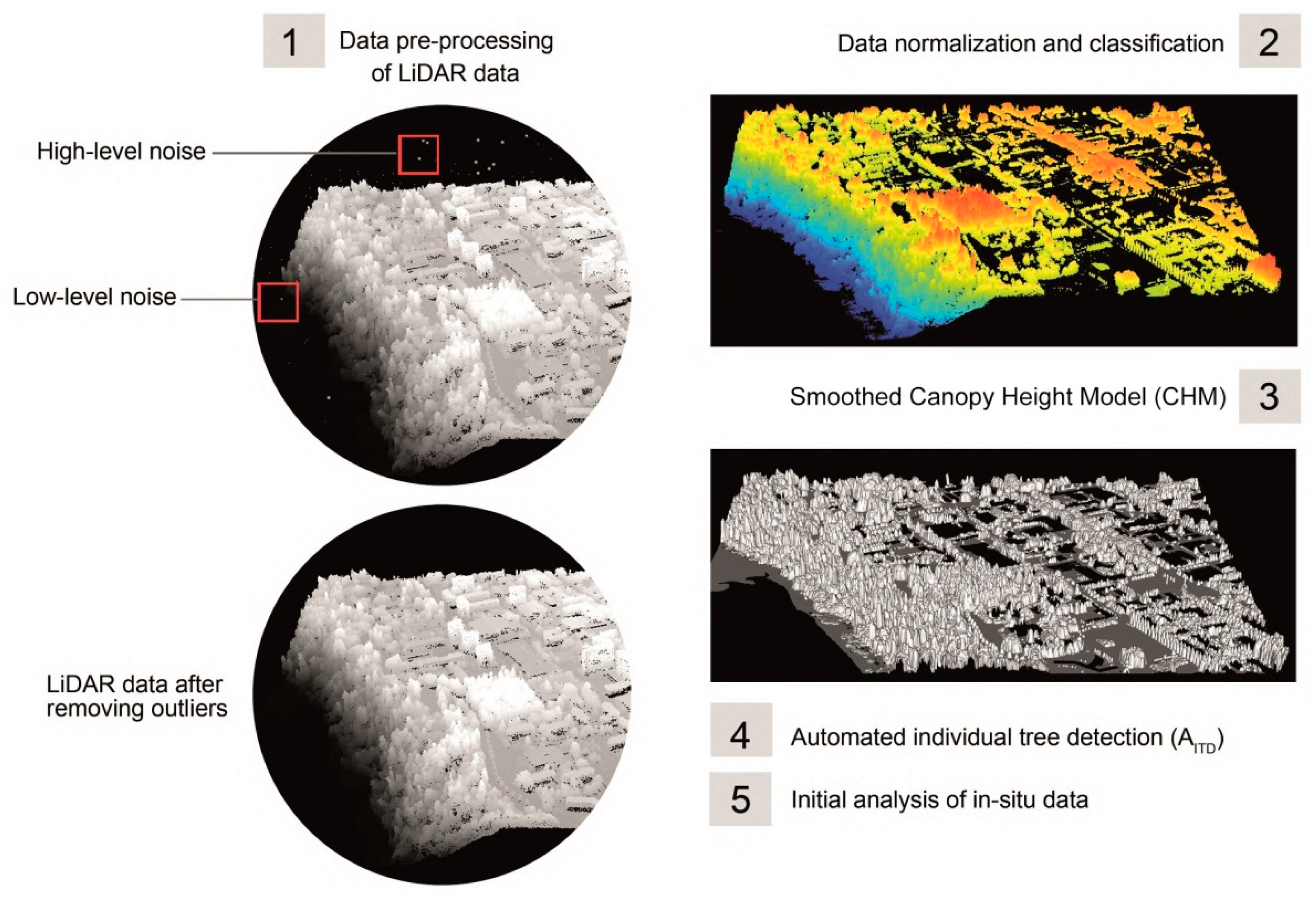
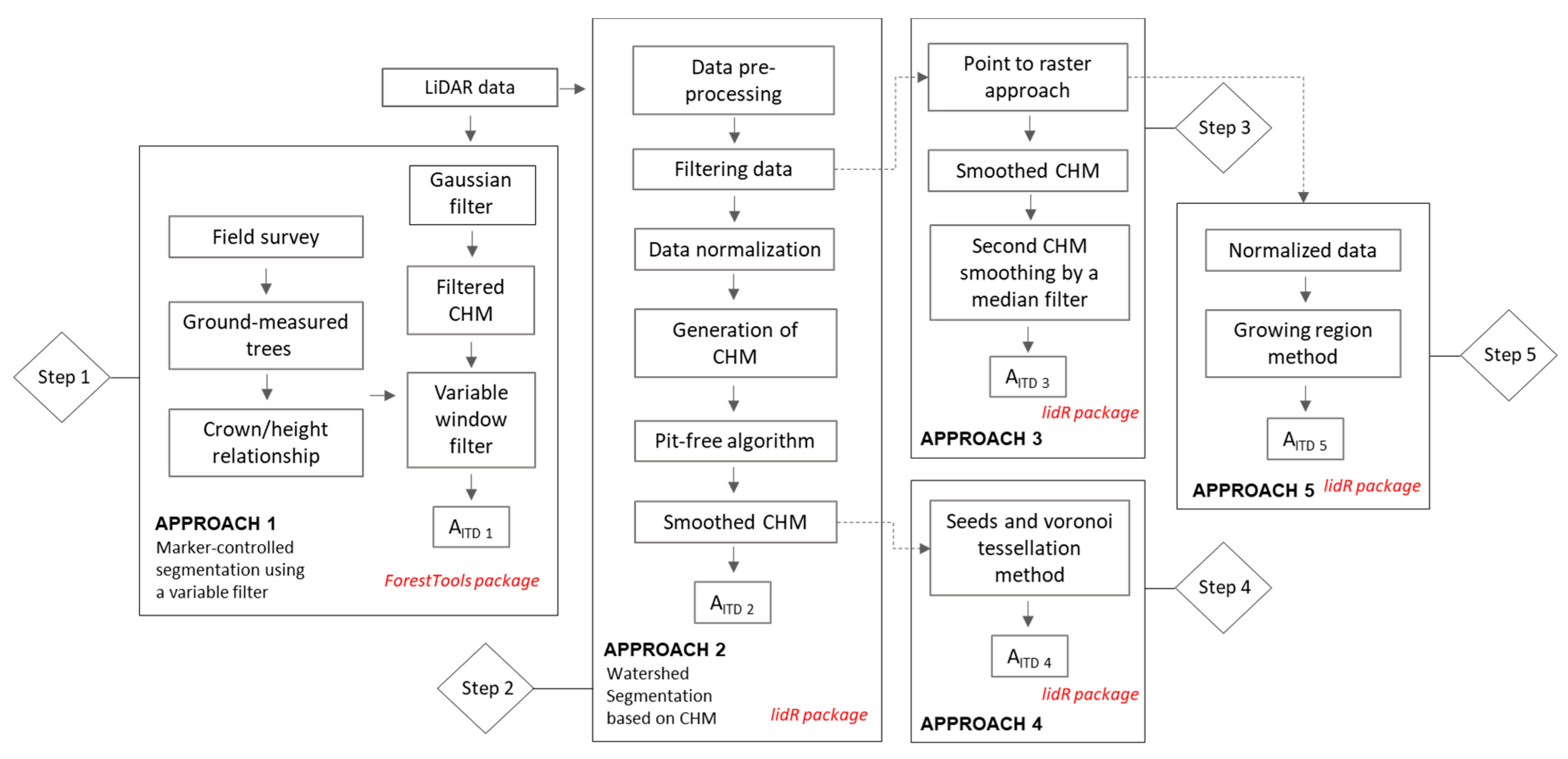
The primary objective for the methodology used for this study was to develop a workflow that would be the basis for quantifying the carbon storage in urban trees using LiDAR data (Figure 3).
Five stages of the analysis were identified, as shown in Figure 3: (1) data pre-processing including filtering, (2) data normalization and classification of high vegetation, (3) generation of a smoothed canopy height model (CHM), (4) automated individual tree detection (AITD) techniques, and (5) initial analysis of ground-measured data. Identifying and extracting tree information from LiDAR data was challenging, especially when the trees were standing as a group. Additionally, segmentation approaches were mostly prone to under- or over-segmentation due to differences in tree biometrics. Therefore, choosing an efficient approach was a crucial part of the data analysis. Individual tree segmentation was the most important step of this study, since the success of the segmentation affected the other research steps. For this reason, we divided this part of the project into five steps, as shown in Figure 4.
Since the aim of this study was not to refine the segmentation, we tested five AITD techniques to check and decide which one to utilize according to the segmentation success. Except for the algorithm based on normalized data introduced by Li et al. [56], all AITD methods were based on CHM. The lidR package [57] and ForestTools package [58] designed in R (version 3.6.3.) language of the environment (http://www.r-project.org/) were used to perform AITD algorithms. Marker-controlled watershed segmentation was employed in the ForestTools library of R [58]. These algorithms were chosen according to their high efficiency, especially for studies conducted in the urban environment [41,59,60].
The first approach was marker-controlled watershed segmentation, which began with applying a Gaussian filter, as formulated below, in order to smooth the CHM [55,61].
g ( x , y , σ )   =   1 2 Π σ e ( x 2 + y 2 ) 2 σ 2 ,
where x and y were the distance to the center of the smoothing kernel, s was used to adjust the parameters of the Gaussian function, and a 3 × 3 pixel Gaussian lowpass filter (with the smoothingfilter parameter in the digital forestry toolbox) filtering kernel was applied using the digital forestry toolbox in Matlab 2019b. A variable filter, which was used in parallel with watershed segmentation, was applied to determine locations of treetops [55,62,63]. This algorithm employs a moving window for CHM to filter pixels; the highest value within the window is regarded as a treetop. The size of the window differs and depends on the positive relationship between crown width (CW) and tree height (TH) [59,64]. Here, a set of 60 perfectly segmented sample trees were used to acquire the formula for calculating the size of the moving window. Then, a linear model was fitted to the crown width CW versus TH using R. Using the CW model, a variable window filter was applied to LiDAR-derived CHM, and the locations of treetops were generated. The coefficients of the model were required for using the ForestTools package and for complete marker-controlled watershed segmentation.
C W ( m ) = 0.7 x   TH   ^ ( m )   +   1.42 ,
The locations of treetops were used, and the marker-controlled watershed segmentation algorithm was applied.
In the second step of AITD, the data were pre-processed and noise was filtered from the point cloud. High-level outliers (called noise) caused by high-flying objects such as birds or aircraft were eliminated from LiDAR data. A simple way to detect outliers was to measure the 95th percentile of height in 10 × 10 m pixels and then remove the points that were above the 95th percentile. Next, an algorithm (knnidw) for spatial interpolation was used to generate a LiDAR-derived digital terrain model (DTM). The interpolation was done using a k-nearest neighbor (KNN) approach with an inverse distance weighting (IDW), and LiDAR data were normalized. CHMs derived from LiDAR data were used to extract tree parameters. For producing CHM, a pit-free algorithm was used, as introduced by Khosravipour et al. [65]. This algorithm uses different heights and is based on the computation of a set of classical triangulations. The sub-circle in the pit-free algorithm enables virtual emulation in the data so that the CHM gets smoother and has fewer empty pixels. The second smoothing process was the application of a median filter to eliminate imitated local maxima caused by tree branches. The filter enables the determining of the boundary of the tree canopy and gives better results prior to AITD. Next, 5 × 5 and 3 × 3 moving windows were applied, and the 5 × 5 fixed window was chosen on the basis of a better result. Following this step, simple watershed segmentation was applied. This procedure utilizes smoothed CHM and individual tree information such as treetop location, TH, CW, and canopy area (CA). According to mathematical morphology, watershed segmentation is an approach that regards an image as a topographic landscape with ridges and valleys [55,66,67]. This method uses morphological similarity and finds the valleys between the crowns in CHM using elevation values.
The LidR R package was used in the third step for segmentation on a CHM (point-to-raster method, resolution 1 m). The CHM was smoothed by surrounding each point with eight points within a 10 cm radius, and then smoothed further with a median filter. The Dalponte algorithm was employed after computing tree positions using a local maximum filter [68]. Then, after mapping the convex hulls, all the trees in the study area were arrayed in a polygon shapefile.
In the fourth step, a method based on seed and Voronoi tessellation (equivalent to nearest neighbor) by Silva et al. [69] was applied. In the last step, a top-to-bottom region growing method developed by Li et al. [56] was applied directly to the LiDAR normalized point cloud. This method depends on the relative spacing between trees, and segmentation is done individually and sequentially from the tallest to the shortest [56].
Each AITD has specific input parameters. For instance, while Dalponte and Coomes [68] used growing thresholds (th_seed and th_cr) and crown diameter threshold (max_cr), Silva et al. [69] used maximum CW as a proportion of TH (max_cr_factor), and pixels with elevation lower than exclusion were multiplied by the TH (exclusion). In other words, input parameters and their complexity differ from each other. We employed several trials, and the input parameters were determined by trial and error for each AITD.
In summary, dendrological parameters were derived from both ground-measured and LiDAR data. Five AITD algorithms were tested comparatively, and two nonlinear models (nls) were developed for this study. At the modeling step, a threshold for canopy width (CW) was applied with five different values to find the most appropriate Akaike’s information criterion (AIC) and log-likelihood value of nls models.
After AITD, an accuracy assessment of each AITD was done. To do this, true positive (correctly segmented) and false positive segments were taken into consideration. Selection of the most suitable AITD routine was based on the accuracy assessment (Figure 5). Using the tree species recorded in the campus GIS database, CW was computed for each individual tree. CW was then used to produce a circular centroid for each tree’s point location. Although the circles that were drawn taking the reference of centroids were not close to the actual shape of tree crowns, they were useful to detect basic errors in tree detection algorithms. Test segments were compared to the reference circles, and errors were recorded using the following set of rules [58]: (1) if none of the test segments had ≥50% of its area within a reference circle, it was considered that the tree corresponding to that circle was missed by the algorithm; (2) in the case that a test segment had ≥50% of its area within a reference circle, an error of commission was recorded as the tree was considered as overly segmented; (3) in the case that a test segment covered ≥50% of the area of more than a single reference circle, trees corresponding to these circles were considered as included within a single element, thus indicating an error of omission (Figure 5).
The number of matched trees (MT) characterizes the segmentation quality; the number of omission errors (OE) and commission errors (CE) represents the under- and over-segmentation, respectively. The accuracy of the method was evaluated in terms of recall (Re), precision (Pr) and F-score (F) using the following equations [70]:
R e = M T M T + O E ,
P r = M T M T + C E ,
F = 2 × R e   × P r R e +   P r
where Re represents a measure of tree detection rate, Pr is a measure of correctness of detected trees, and F is a measure of overall accuracy, taking CE and OE into account.

2.3. DBH and Carbon Models

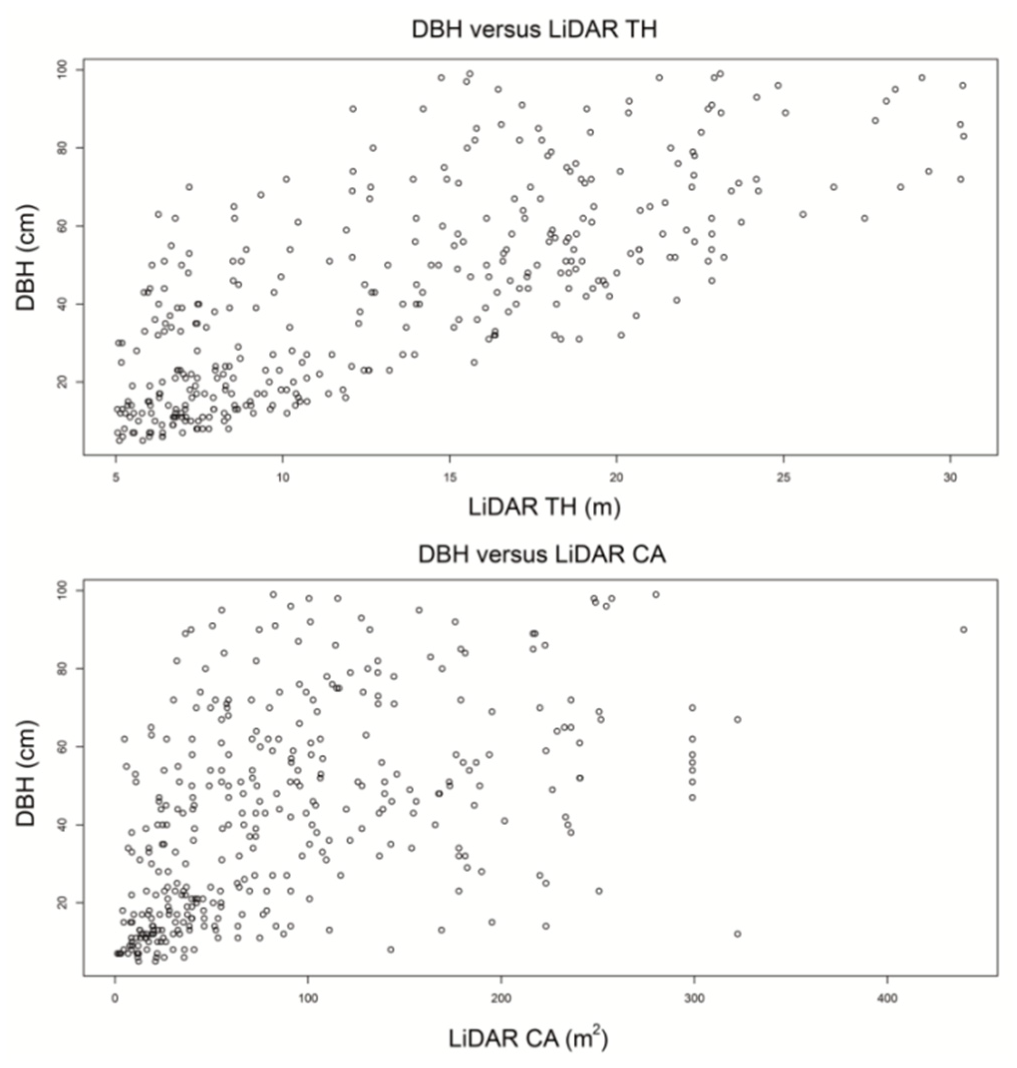
The DBH of trees is strongly related to the other allometry characteristics (tree measurements), including TH and crown metrics [71]. It is also one of the most common variables measured in urban forests [72]. For each tree of this study, the CA and maximum TH were obtained using the LiDAR data and applying the Dalponte algorithm. Next, the allometric measures from the subset of ground-measured trees were intersected with LiDAR-derived trees in ArcMap 10.7 and used to develop DBH estimation models. Where ground-measured trees were not spatially well matched with segmented LiDAR trees, they were not used for the DBH models. Using the remaining 363 trees, the first graphs of DBH versus LiDAR CA and maximum TH were obtained. The graphs showing DBH versus LiDAR CA and TH were plotted in R (Figure A1) and a non-linear model was chosen (Figure A2). We used the DBH estimation model presented in Equation (6).
DBH ^ = b 1 × ( ( TH 1.3 ) b 2 ) × ( CA b 3 ) ,
where DBH is the ground-measured DBH (cm), TH is the LiDAR maximum TH (m), CA is the LiDAR crown area (m2), and b1 to b3 are parameters to be estimated.
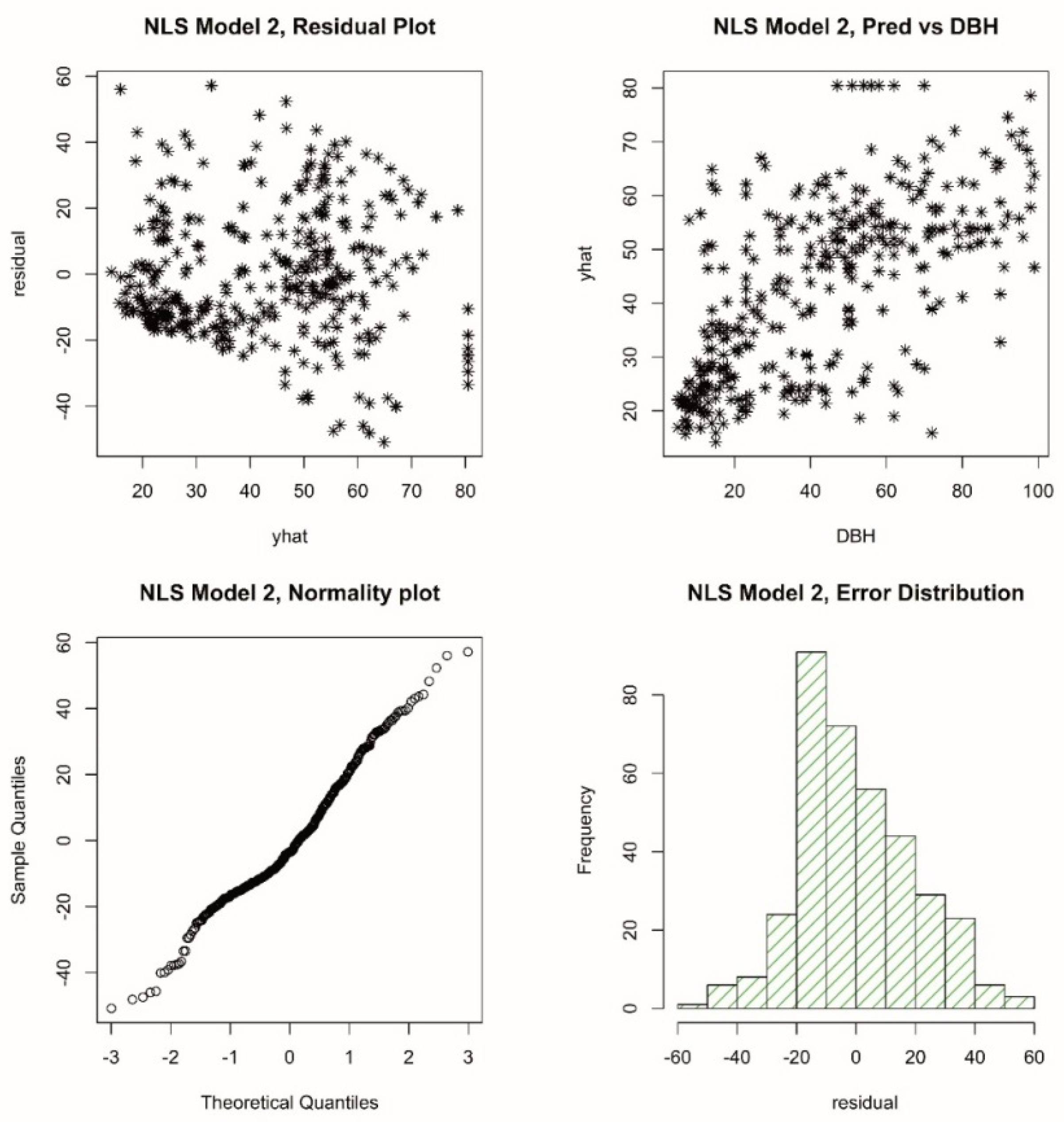
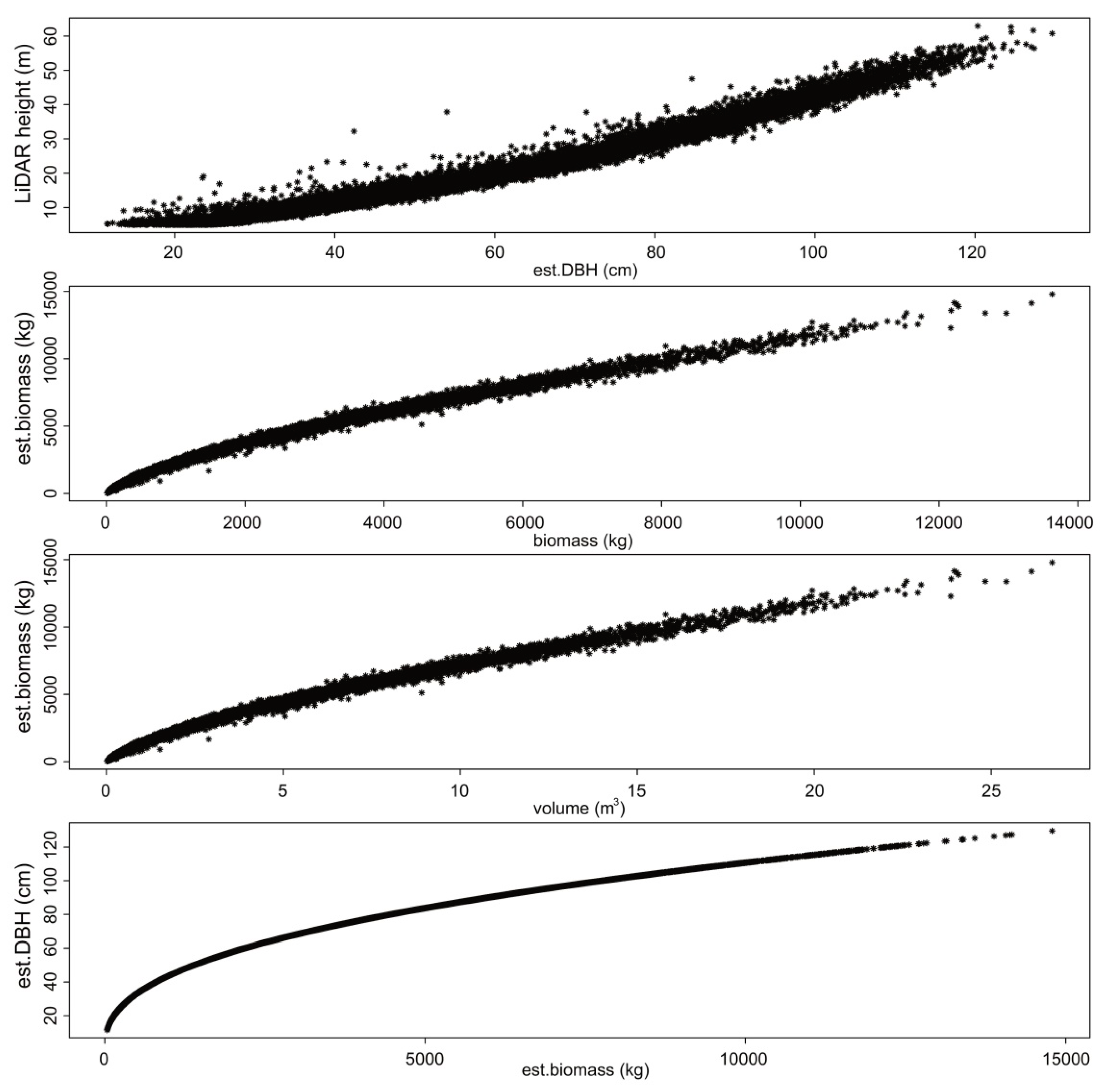
The use of TH-1.3 in the model in Equation (6) is flexible, representing a wide variety of nonlinear trends. The model presumes that the estimated DBH is 0, when the TH height is 1.3 m. Subsequently the nlin( ) function of R was used to fit the model, using CA calculated from five different CW thresholds (th) depending on the max_cr (maximum value of the crown diameter of a detected tree) parameter of the Dalponte algorithm. Starting parameters were varied to ensure a global optimum for the estimated model parameters. Then, the five models were compared using Akaike’s information criterion (AIC), log-likelihood, and root-mean-squared error, and one model was recommended for use. Final checks were made for accuracy of the used model (Figure A3). Here, using the biomass model with the estimated DBH, and comparing this with a quick estimated biomass (via a quick tree volume estimation using 510 kg/m3 volume (the value for Douglas fir), we checked the estimated biomass values, particularly for trees above 50 m.
Using the selected model, DBH was estimated for each LiDAR tree. The estimated DBH was then utilized to estimate above-ground carbon (cag) using an existing biomass model and assuming thar 0.50 of biomass is carbon [14,73,74].
c a g   ^ = 0.50 × ( exp   ( a + b × ln   DBH ^ ) ) ,
where a and b are estimated parameters, c a g ^ is the estimated tree above-ground carbon (kg), and DBH ^ is the estimated DBH (cm).
Although Schreyer et al. [14] highlighted that a and b vary by genera and species, as well as growth conditions, they used only one set of estimated parameters given the large number of species in their study area. Similarly, given the very large number of tree species in this university urban forest, the parameter estimates given by Jenkins et al. [75] (a = −2.48 and b = 2.4835) developed for mixed deciduous forests of the United States of America (USA) were used in this study. Once the above-ground carbon was estimated for each tree, the study area carbon was estimated. The overall workflow for estimating carbon is given in Figure 6.

3. Results

Results show that using different estimates of AITD was an efficient way of preventing time-consuming segmentation refinement. Selecting the best accuracy of the tree segmentation enabled a quick result when the segmentation algorithm have a higher accuracy than 80%.

3.1. Segmentation and Accuracy Assessment Results

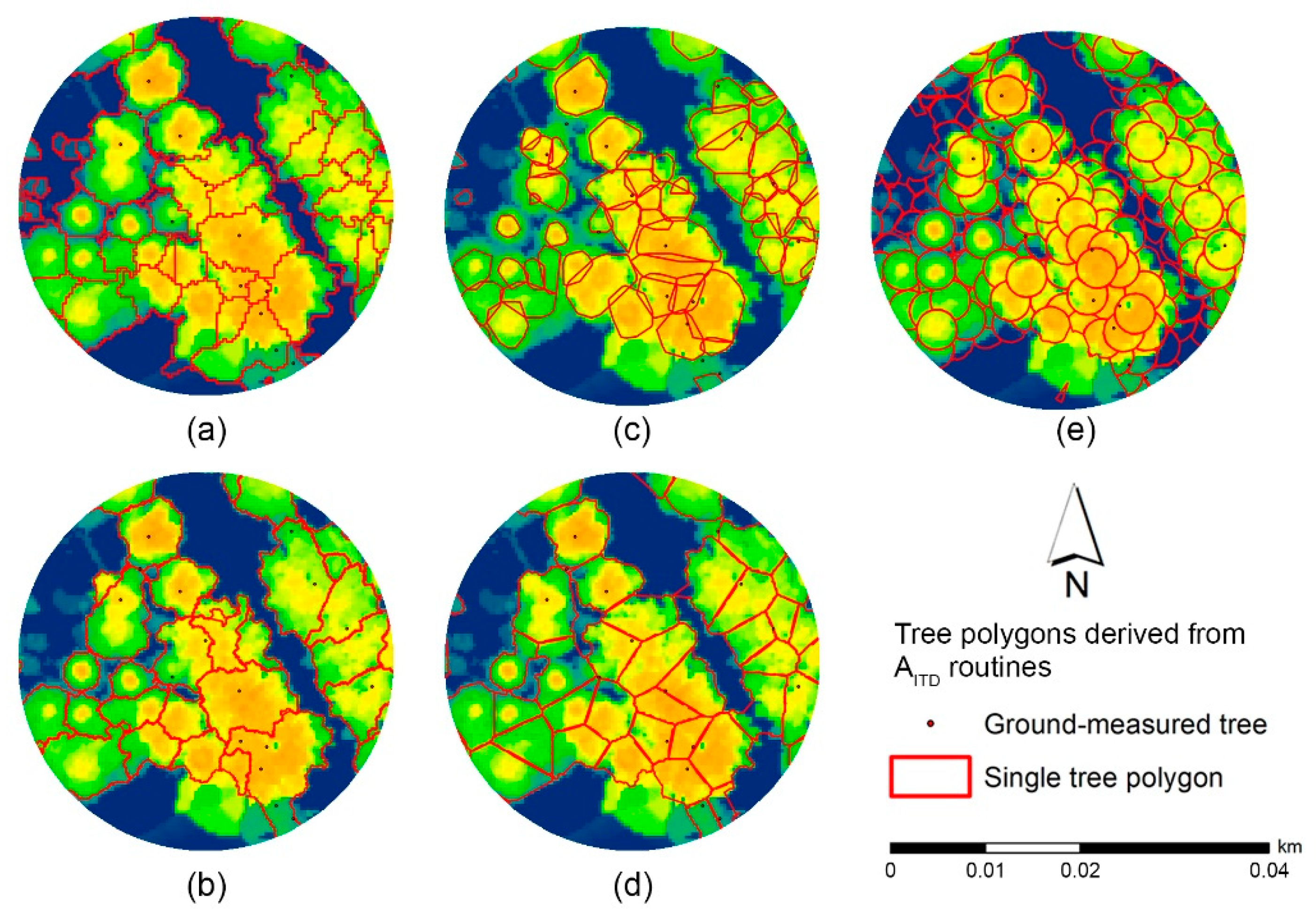
Marker-controlled watershed segmentation and AITD by Li et al. [64] had an over-segmentation problem, while the other AITD had under-segmentation problems (Figure 7).
One common issue for any segmentation algorithm is the number of omissions (missing trees) and commissions (extra trees). A total of 300 ground-located trees were used for an accuracy assessment of these five algorithms. Although the F scores were similar, the Dalponte algorithm had the highest accuracy (F score = 0.83) and was selected (Table 1).

3.2. DBH Model and Carbon Estimates

A total of 363 ground-measured trees with matching LiDAR measures were used to develop the DBH models. Five CA alternatives based on varying the max_cr parameter of the Dalponte algorithm were tested for this model. Specifically, max_cr values of 10, 15, 20, 25, and 30 were compared. First, increasing max_cr above 25 resulted in the same AIC and log-likelihood values (Table 2). A max_cr = 20 gave the best results (smallest AIC and root-mean-squared errors and largest log-likelihood), better than using the default value of 10 used in the segmentation algorithm.
The selected model was, therefore,
DBH ^ = 6.6597 × ( ( TH 1.3 ) 0.6145 ) × ( CA 0.0817 ) ,
where CA was obtained using max_cr = 20. The Dalponte algorithm was applied with max_cr = 20, and a final wall-to-wall segmentation was completed using the lidR R package before producing the carbon storage map.
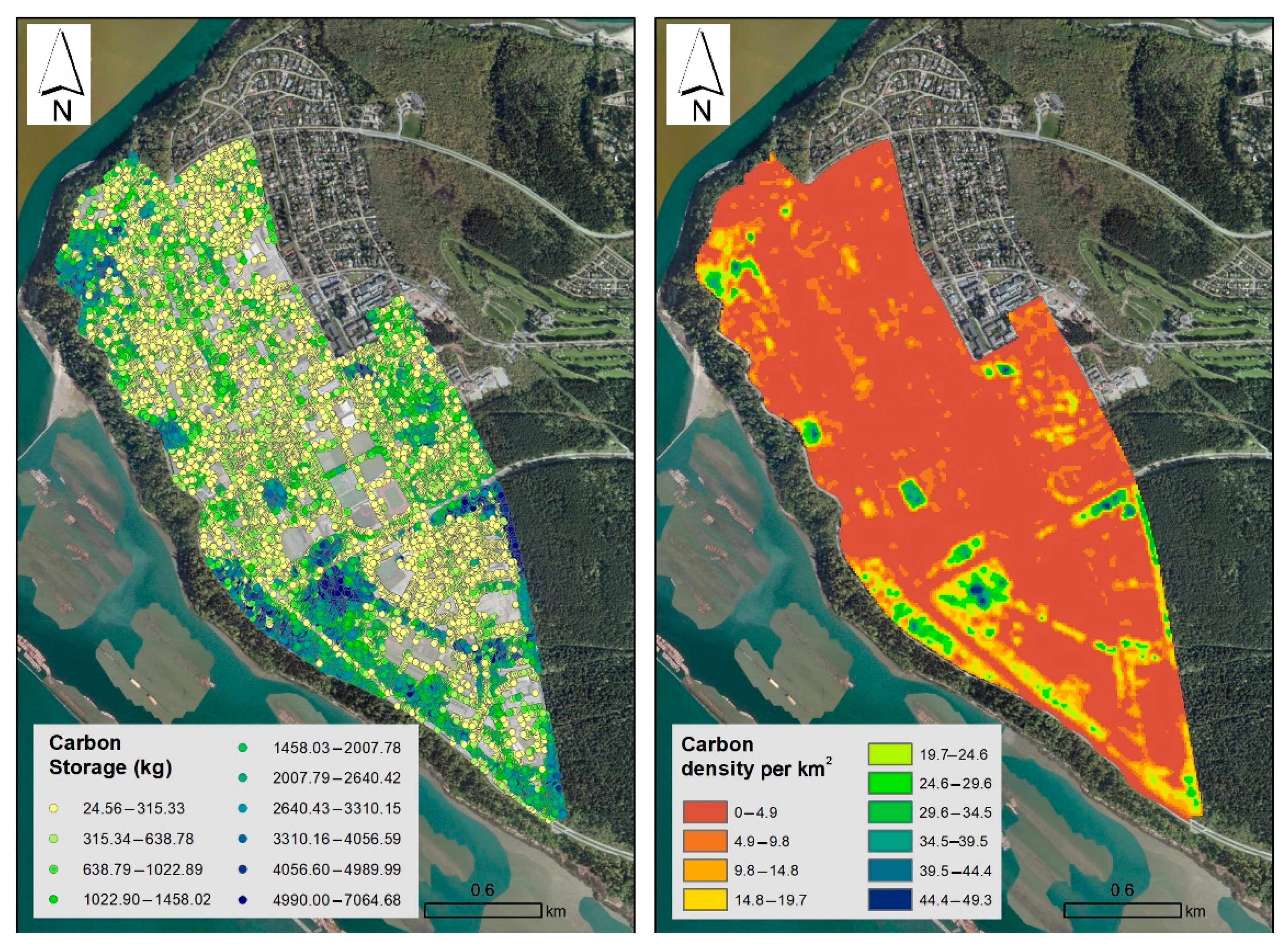
Trees higher than 5 m were delineated on the main campus of UBC using the Dalponte algorithm, and the maximum TH and CA were calculated for each tree. From this result, the DBH values were estimated. For each tree, the DBH was estimated and used to estimate the tree carbon. Figure 8 presents a kernel density map of above-ground tree carbon storage per km2 (kg/km2), along with the estimated carbon of each tree.
The results of this case study show the usability of RS techniques to assess carbon storage in an urban environment. In addition, the results demonstrate that there are differences in carbon storage between different structural units at the main campus of UBC. According to the estimation of carbon density, total carbon storage was estimated at 21.174 Mg (5.27 kg C·m−2). University land types are often considered a homogeneous land use type (i.e., “institutional”) but the types are designed and used for different purposes. In the same vein, universities also have potential as living laboratories, which makes them worthy of further in-depth study. When results were combined with the land-use map of UBC, it was seen that the amount of carbon storage varied across the campus. The highest percentage of carbon storage was found in the campus area under academic use (75.16%). This was followed by campus areas with residential areas (20.62%). The part of the campus allocated to future residential areas had the lowest amount of carbon storage (4.22%).

4. Discussion

In this case study, we proposed a methodological approach to estimate above-ground carbon storage of urban trees using LiDAR data based on an nls model. Our results suggest that LiDAR data help to quantify the carbon storage of trees at urban level. The costs of estimating the ecosystem services that urban trees provide can be greatly reduced by RS data and approaches. The main goal of the present study was to develop an efficient and effective RS-based strategy to estimate the above-ground carbon storage of urban trees using LiDAR data coupled with a sample of ground measures in an urban environment.
Detection of individual trees in a LiDAR-based urban vegetation study is both challenging and important. The sometimes complex shapes of the crowns can lead to errors in representing individual trees. Nevertheless, in this study, there was strong agreement between the RS analysis and field data. Relative homogeneity of vegetation within subareas, in contrast to the overall study area, contributed to the level of accuracy attained. The algorithms employed in this study are not free from possible sources of error. Small trees could be missed (e.g., classified as branches) if they are close to big trees and, thus, omitted by the treetop removal procedure. Exceptionally large trees might have crowns that spread so much that their branches are falsely identified as treetops, leading to overestimations [16].
The segmentation accuracy (F-score) of the Dalponte algorithm was the highest of all the AITD algorithms. One of the possible reasons could be the second smoothing of CHM by a median filter. Another reason could be the local maximum filter that was applied after the second smoothing of CHM. Although the LiDAR data used had high point density and the methods were efficient, the following limitations pertain to this study: (1) AITD resulted in some extra trees and some missing trees in the LiDAR trees dataset; (2) when LiDAR-derived crowns intersected with ground-measured data, there were some mismatched trees; (3) in spite of an extensive search, no existing biomass models were found for many of the urban tree species of the study area. When ground-measured trees were matched with LiDAR-derived trees to develop a DBH estimation model, it was found that some trees were not well matched. Since this study did not aim to refine segmentation and included 22 missing trees, the first limitation was disregarded. In addition, LiDAR-based estimation tends to underestimate or overestimate tree attributes due to the divergent laser pulses [76]. Moreover, it should be noted that there was a gap of approximately 1 year 4 months between the LiDAR and field surveys, which may have resulted in estimation errors. With respect to mismatched trees, the literature has discussed that canopy conditions can lead to “false” trees [77]. When looking at the third study limitation, species substitution was needed, which may not give accurate AGB estimates. The UBC tree species information was produced in 1998 and has not been updated since 2008. Therefore, species information was limited, and constants for species were not applicable. From the field survey, it was observed that exotic species were much more dominant than native species, including species representing the genera Quercus, Fagus, Magnolia, Cedrus, Taxus, and Tilia. Among native species, the Acer genus was the most dominant. Arbutus, Betula, Cornus, Crataegus, Cupressus, Pinus, Populus, and Prunus were other genera of exotic species identified in the field survey. Schreyer et al. [14] found that these genera were indicated by Jenkins’ constants (−2.48 and 2.4835) for mixed deciduous forests of the US [75]. Since growth conditions were similar to Jenkins’ study area, it was assumed that the constants were the best option for the main campus of UBC Vancouver. Given that there was limited information of species, cag was quantified by multiplying the AGB rate by 0.5.
To distinguish among stacked (suppressed) trees, it proved to be a simple, effective method to employ various thresholds based on CW, one that should be applicable to multilayer forests. The choice of thresholds is based on characteristics and uncertainties associated with the input data. Visual assessment and calibration should be undertaken before completing the validation. It was assumed that tuning parameters of AITD could result in different findings, and this could influence the success of the estimation model. On the other hand, it was understood that selecting an inappropriate th value caused an omission or commission error. Therefore, finding the correct th value was challenging and there was no routine to pick the most appropriate value. All parameters were applied several times to choose the correct th, and max_cr showed an important effect on tree detection. When all models that were developed for this study were compared, it was found that AIC and log-likelihood values were changing according to the different max_cr values, and final results presented in this case study demonstrate that using different max_cr of the tree segmentation algorithm can result in higher efficiency for developing estimation models. Interestingly, when the th for max_cr was above 25, AIC, Log-Lik, and RMSE were the same. Since th 25 and th 30 gave the same results, we did not continue to test th above 30. Here, we did not classify the tree species on the basis of similarities in allometry characteristics, and we did not use the different values for different classes to reduce the bias. However, further study can focus on the variation between tree species to make more accurate carbon estimations.
In this study, DBH models had a limited height range relative to the entire LiDAR tree data. This means that this model may not do well for taller heights, especially above 50 m tall. This can be explained by the high growing site conditions in the campus. In Figure A3, overestimation of biomass can be explained by either AITD issues (such as under- and over-segmentation) or growing conditions of tall trees.
Estimates of C density in urban forests from the few examples given in the introduction of this paper ranged from 1.1 kg C·m−2 (Leipzig [25]) to 7.69 kg C·m−2 (US cities average [17]). In this study, the UBC campus yielded an estimate of 5.27 kg C·m−2, well within the range of the other estimates, and probably rather high for the latitude of the campus.
These results demonstrate the potential for more extensive (e.g., citywide) estimates of carbon storage and climate mitigation, as well as comparative studies across urban environments and over time. The methodology will support better environmental planning and design, including policy and management measures related to climate change and urban resilience. More detailed information for various tree species, including allometric constants and region-specific growth estimates would support more accurate analyses and more confident assessments. Incorporation of growth parameters in urban forest models will support estimates of carbon storage as a dynamic process, beyond our current inventories of biomass and carbon density.

5. Conclusions

This study compared five AITD algorithms at a university campus in order to estimate above-ground carbon storage. The results showed that, although there was a slight difference between F-scores, the Dalponte algorithm performed best with the highest F-score (0.83). Of the five CW thresholds (th) tested in the DBH estimation model, using th = 20 resulted in the lowest Akaike’s information criterion (AIC), the highest log-likelihood, and the lowest RMSE (19.55 cm). Above-ground carbon was estimated for each tree in the study area and subsequently summarized, resulting in an estimated 5.27 kg C·m−2 over the main campus of UBC, Vancouver. The approach could be used in other urban jurisdictions to obtain essential information on urban carbon storage in support of urban landscape governance, planning, and management.
The planners and managers of urban trees are tasked with planting and taking care of urban vegetation in often harsh, high-pressure urban environments. This task becomes particularly daunting during times of continuing urbanization and development. Even in the densest urban environments, trees are needed because of the many ecosystem services they provide, including contributions to climate change mitigation and adaptation. With focus on carbon storage by trees, this is well illustrated in our study by the rapidly developing UBC campus. The methodological approach provides cost-effective and useful information according to various algorithms that apply various thresholds and, therefore, can be used effectively as a reference for further studies.
Decisions about the planning and management of urban landscapes need to be based on sound evidence, including assessment of urban vegetation and the ecosystem services it provides. Moreover, assessment methods need to be easy to use for decision-makers and be realistic and cost-efficient in terms of data collection requirements. This paper introduced a LiDAR-based approach to support the assessment of one specific ecosystem service, namely, carbon storage by urban trees. The methodology presented in this paper for assessing the AGB of urban trees contributes to the search for more efficient and effective approaches that can be used in planning and management. Further research and testing are needed to refine the methodology and implement it in an actual landscape planning and management context. Moreover, assessment of carbon storage by urban trees needs to be carefully integrated with the assessment of other ecosystem services. More complete information about the allometry and growth rates of various species of urban trees would confer greater accuracy in these assessments.

Author Contributions

Conceptualization, D.G.; methodology, D.G.; software, D.G.; analysis, D.G.; investigation, D.G.; resources, D.G.; data curation, D.G.; writing—original draft preparation, D.G.; writing—review and editing C.C.K.v.d.B. and D.G.; visualization, D.G.; supervision, C.C.K.v.d.B.; project administration, C.C.K.v.d.B. and D.G.; funding acquisition, D.G. All authors have read and agreed to the published version of the manuscript.

Funding

The authors are indebted to the Scientific and Technological Research Council of Turkey for their financial support under the 2219 program.

Acknowledgments

Colleagues at the Urban Forest Research in Action Lab, Faculty of Forestry, UBC are thanked for their contributions to this work. Valerie LeMay is specially thanked for her support in developing the nls model used in this study. We would like to thank the anonymous reviewers for their constructive comments and suggestions.

Conflicts of Interest

The authors declare no conflict of interest.

Appendix A

Table A1. List of abbreviations used in the manuscript along with their full forms.
AbbrevationFull Form
AGBAbove-ground carbon
AITDAutomated individual tree detection
CCarbon
CALiDAR canopy area
CHMCanopy height model
CWLiDAR crown width
DBHDiameter of outside bark at breast height
DTMDigital terrain model
ESEcosystem services
GIGreen ınfrastructure
KNNk-nearest neighbor
LiDARLight detection and ranging
MTHMeasured tree height
RSRemote sensing
THLiDAR tree height
ththreshold
UBCUniversity of British Columbia
Figure A1. The relationship between LiDAR TH/LiDAR CA and DBH.
Forests 12 00062 g0a1
Figure A2. Diagnostic plot for the nls model.
Forests 12 00062 g0a2
Figure A3. Final checks for the used model.
Forests 12 00062 g0a3

References

  1. Nowak, D.J.; Crane, D.E.; Stevens, J.C.; Hoehn, R.E.; Walton, J.T.; Bond, J. A ground-based method of assessing urban forest structure and ecosystem services. Aboriculture Urban For. 2008, 34, 347–358. [Google Scholar]
  2. Niemelä, J.; Saarela, S.R.; Söderman, T.; Kopperoinen, L.; Yli-Pelkonen, V.; Väre, S.; Kotze, D.J. Using the ecosystem services approach for better planning and conservation of urban green spaces: A Finland case study. Biodivers. Conserv. 2010, 19, 3225–3243. [Google Scholar] [CrossRef]
  3. Manes, F.; Incerti, G.; Salvatori, E.; Vitale, M.; Ricotta, C.; Costanza, R. Urban ecosystem services: Tree diversity and stability of tropospheric ozone removal. Ecol. Appl. 2012, 22, 349–360. [Google Scholar] [CrossRef] [PubMed]
  4. Bolliger, J.; Silbernagel, J. Contribution of connectivity assessments to Green Infrastructure (GI). ISPRS Int. J. Geo Inf. 2020, 9, 212. [Google Scholar] [CrossRef] [Green Version]
  5. Gill, S.E.; Handley, J.F.; Ennos, A.R.; Pauleit, S. Adapting cities for climate change: The role of the green infrastructure. Built Environ. 2007, 33, 115–133. [Google Scholar] [CrossRef] [Green Version]
  6. Foster, J.; Lowe, A.; Winkelman, S. The value of green infrastructure for urban climate adaptation. Center Clean Air Policy 2011, 750, 1–52. [Google Scholar]
  7. Hostetler, M.; Allen, W.; Meurk, C. Conserving urban biodiversity? Creating green infrastructure is only the first step. Landsc. Urban Plan. 2011, 100, 369–371. [Google Scholar] [CrossRef]
  8. Pugh, T.A.M.; MacKenzie, A.R.; Whyatt, J.D.; Hewitt, C.N. Effectiveness of green infrastructure for improvement of air quality in urban street canyons. Environ. Sci. Technol. 2012, 46, 7692–7699. [Google Scholar] [CrossRef] [PubMed] [Green Version]
  9. Ellis, J.B. Sustainable surface water management and green infrastructure in UK urban catchment planning. J. Environ. Plan. Manag. 2013, 56, 24–41. [Google Scholar] [CrossRef]
  10. Baldauf, R.; McPherson, G.; Wheaton, L.; Zhang, M.; Cahill, T.; Bailey, C.; Fuller, C.H.; Withycombe, E.; Titus, K. Integrating vegetation and green infrastructure into sustainable transportation planning. Transp. News 2013, 288, 14–18. [Google Scholar]
  11. van den Bosch, M.; Nieuwenhuijsen, M. No time to lose–Green the cities now. Environ. Int. 2017, 99, 343–350. [Google Scholar] [CrossRef] [PubMed]
  12. Nowak, D.J.; Crane, D.E. Carbon storage and sequestration by urban trees in the USA. Environ. Pollut. 2002, 116, 381–389. [Google Scholar] [CrossRef]
  13. Lewis, S.L.; Lopez-Gonzalez, G.; Sonké, B.; Affum-Baffoe, K.; Baker, T.R.; Ojo, L.O.; Phillips, O.L.; Reitsma, J.M.; White, L.; Comiskey, J.A.; et al. Increasing carbon storage in intact African tropical forests. Nature 2009, 457, 1003–1006. [Google Scholar] [CrossRef] [PubMed]
  14. Schreyer, J.; Tigges, J.; Lakes, T.; Churkina, G. Using airborne LiDAR and QuickBird data for modelling urban tree carbon storage and its distribution-a case study of Berlin. Remote Sens. 2014, 6, 10636–10655. [Google Scholar] [CrossRef] [Green Version]
  15. Velasco, E.; Chen, K.W. Carbon storage estimation of tropical urban trees by an improved allometric model for aboveground biomass based on terrestrial laser scanning. Urban For. Urban Green. 2019, 44, 126387. [Google Scholar] [CrossRef]
  16. Zhang, C.; Zhou, Y.; Qiu, F. Individual tree segmentation from LiDAR point clouds for urban forest inventory. Remote Sens. 2015, 7, 7892–7913. [Google Scholar] [CrossRef] [Green Version]
  17. Nowak, D.J.; Greenfield, E.J.; Hoehn, R.E.; Lapoint, E. Carbon storage and sequestration by trees in urban and community areas of the United States. Environ. Pollut. 2013, 178, 229–236. [Google Scholar] [CrossRef] [Green Version]
  18. Giannico, V.; Lafortezza, R.; John, R.; Sanesi, G.; Pesola, L.; Chen, J. Estimating stand volume and above-ground biomass of urban forests using LiDAR. Remote Sens. 2016, 8, 339. [Google Scholar] [CrossRef] [Green Version]
  19. Tigges, J.; Churkina, G.; Lakes, T. Modeling above-ground carbon storage: A remote sensing approach to derive individual tree species information in urban settings. Urban Ecosyst. 2017, 20, 97–111. [Google Scholar] [CrossRef]
  20. Myeong, S.; Nowak, D.J.; Duggin, M.J. A temporal analysis of urban forest carbon storage using remote sensing. Remote Sens. Environ. 2006, 101, 277–282. [Google Scholar] [CrossRef]
  21. Davies, Z.G.; Edmondson, J.L.; Heinemeyer, A.; Leake, J.R.; Gaston, K.J. Mapping an urban ecosystem service: Quantifying above-ground carbon storage at a city-wide scale. J. Appl. Ecol. 2011, 48, 1125–1134. [Google Scholar] [CrossRef] [Green Version]
  22. Pasher, J.; McGovern, M.; Khoury, M.; Duffe, J. Assessing carbon storage and sequestration by Canada’s urban forests using high resolution earth observation data. Urban For. Urban Green. 2014, 13, 484–494. [Google Scholar] [CrossRef]
  23. Raciti, S.M.; Hutyra, L.R.; Newell, J.D. Mapping carbon storage in urban trees with multi-source remote sensing data: Relationships between biomass, land use, and demographics in Boston neighborhoods. Sci. Total Environ. 2014, 500, 72–83. [Google Scholar] [CrossRef] [PubMed]
  24. Hutyra, L.R.; Yoon, B.; Alberti, M. Terrestrial carbon stocks across a gradient of urbanization: A study of the Seattle, WA region. Glob. Chang. Biol. 2011, 17, 783–797. [Google Scholar] [CrossRef]
  25. Strohbach, M.W.; Haase, D. Above-ground carbon storage by urban trees in Leipzig, Germany: Analysis of patterns in a European city. Landsc. Urban Plan. 2012, 104, 95–104. [Google Scholar] [CrossRef]
  26. Wilkes, P.; Disney, M.; Vicari, M.B.; Calders, K.; Burt, A. Estimating urban above ground biomass with multi-scale LiDAR. Carbon Balance Manag. 2018, 13, 10. [Google Scholar] [CrossRef]
  27. Yang, Q.; Su, Y.; Jin, S.; Kelly, M.; Hu, T.; Ma, Q.; Li, Y.; Song, S.; Zhang, J.; Xu, G.; et al. The influence of vegetation characteristics on individual tree segmentation methods with airborne LiDAR data. Remote Sens. 2019, 11, 2880. [Google Scholar] [CrossRef] [Green Version]
  28. Duncanson, L.; Armston, J.; Disney, M.; Avitabile, V.; Barbier, N.; Calders, K.; Falkowski, M. The importance of consistent global forest aboveground biomass product validation. Surv. Geophys. 2019, 40, 979–999. [Google Scholar] [CrossRef] [Green Version]
  29. Lambert, M.C.; Ung, C.H.; Raulier, F. Canadian national tree aboveground biomass equations. Can. J. For. Res. 2005, 35, 1996–2018. [Google Scholar] [CrossRef]
  30. He, Y.; Weng, Q. High Spatial Resolution Remote Sensing: Data, Analysis and Applications; CRC Press: Boca Raton, FL, USA, 2018. [Google Scholar] [CrossRef]
  31. Lee, J.H.; Ko, Y.; McPherson, E.G. The feasibility of remotely sensed data to estimate urban tree dimensions and biomass. Urban For. Urban Green. 2016, 16, 208–220. [Google Scholar] [CrossRef] [Green Version]
  32. van Leeuwen, M.; Nieuwenhuis, M. Retrieval of forest structural parameters using LiDAR remote sensing. Eur. J. For. Res. 2010, 129, 749–770. [Google Scholar] [CrossRef]
  33. Zhu, Z.; Zhou, Y.; Seto, K.C.; Stokes, E.C.; Deng, C.; Pickett, S.T.A.; Taubenböck, H. Understanding an urbanizing planet: Strategic directions for remote sensing. Remote Sens. Envion. 2018, 228, 164–182. [Google Scholar] [CrossRef]
  34. Campbell, L.; Coops, N.C.; Saunders, S.C. LiDAR as an Advanced Remote Sensing Technology to Augment Ecosystem Classification and Mapping. J. Ecosyst. Manag. 2017, 17, 1–13. [Google Scholar]
  35. Li, X.; Chen, W.Y.; Sanesi, G.; Lafortezza, R. Remote sensing in urban forestry: Recent applications and future directions. Remote Sens. 2019, 11, 1144. [Google Scholar] [CrossRef] [Green Version]
  36. Guo, X.; Coops, N.C.; Tompalski, P.; Nielsen, S.E.; Bater, C.W.; John Stadt, J. Regional mapping of vegetation structure for biodiversity monitoring using airborne lidar data. Ecol. Inform. 2017, 38, 50–61. [Google Scholar] [CrossRef]
  37. Jaafar, W.S.W.M.; Woodhouse, I.H.; Silva, C.A.; Omar, H.; Maulud, K.N.A.; Hudak, A.T.; Klauberg, C.; Cardil, A.; Mohan, M. Improving individual tree crown delineation and attributes estimation of tropical forests using airborne LiDAR data. Forests 2018, 9, 759. [Google Scholar] [CrossRef] [Green Version]
  38. Popescu, S.C.; Wynne, R.H.; Nelson, R.F. Measuring individual tree crown diameter with lidar and assessing its influence on estimating forest volume and biomass. Can. J. Remote Sens. 2003, 29, 564–577. [Google Scholar] [CrossRef]
  39. Speak, A.; Escobedo, F.J.; Russo, A.; Zerbe, S. Total urban tree carbon storage and waste management emissions estimated using a combination of LiDAR, field measurements and an end-of-life wood approach. J. Clean. Prod. 2020, 256, 120420. [Google Scholar] [CrossRef]
  40. Wang, V.; Gao, J.; Schwendenmann, L. Assessing changes of urban vegetation cover and aboveground carbon stocks using LiDAR and Landsat imagery data in Auckland, New Zealand. Int. J. Remote Sens. 2020, 41, 2140–2158. [Google Scholar] [CrossRef]
  41. Shrestha, R.; Wynne, R.H. Estimating biophysical parameters of individual trees in an urban environment using small footprint discrete-return imaging Lidar. Remote Sens. 2012, 4, 484–508. [Google Scholar] [CrossRef] [Green Version]
  42. Nurhayati, R. Individual Tree Crown Delineation in Tropical Forest Using Object-Based Analysis of Orthoimage and Digital Surface Model. Master’s Thesis, Wageningen University, Wageningen, The Netherlands, 2015. [Google Scholar]
  43. Liu, L.; Coops, N.C.; Aven, N.W.; Pang, Y. Mapping urban tree species using integrated airborne hyperspectral and LiDAR remote sensing data. Remote Sens. Environ. 2017, 200, 170–182. [Google Scholar] [CrossRef]
  44. Trlica, A.; Hutyra, L.R.; Morreale, L.L.; Smith, I.A.; Reinmann, A.B. Current and future biomass carbon uptake in Boston’s urban forest. Sci. Total Environ. 2020, 709, 136196. [Google Scholar] [CrossRef] [PubMed]
  45. Sun, Y.; Xie, S.; Zhao, S. Valuing urban green spaces in mitigating climate change: A city-wide estimate of aboveground carbon stored in urban green spaces of China’s Capital. Glob. Chang. Biol. 2019, 25, 1717–1732. [Google Scholar] [CrossRef] [PubMed]
  46. Teslenko, T. Sustainability on University Campuses: Learning, Skills Building and Best Practices; Springer: Cham, Switzerland, 2019; pp. 3–20. [Google Scholar]
  47. City of Vancouver and Vancouver Park Board. Urban Forest Strategy: 2018. Available online: https://parkboardmeetings.vancouver.ca/2018/20180430/REPORT-UrbanForestStrategy2018Update-20180430.pdf (accessed on 23 February 2020).
  48. Greenhouse Gas Reduction Targets Act. BC Greenhouse Gas Emissions Targets. 2007. Available online: http://www.bclaws.ca/civix/document/id/consol22/consol22/00_07042_01 (accessed on 21 March 2020).
  49. UBC Social Ecological Economic Development Studies (SEEDS) Student Report. UBC 2017 Stadium Neighborhood Tree Inventory Project. Available online: https://sustain.ubc.ca/sites/default/files/seedslibrary/UBC%202017%20Stadium%20Neighbourhood%20Tree%20Inventory%20Project_0.pdf (accessed on 16 December 2020).
  50. UBC Social Ecological Economic Development Studies (SEEDS) Sustainability Program Student Research Report. Campus Urban Forest Inventory and Assessment: Phase 1B University of British Columbia, UFOR 101. Themes: Land, Biodiversity, Climate. Available online: https://open.library.ubc.ca/cIRcle/collections/undergraduateresearch/18861/items/1.0392748 (accessed on 16 December 2020).
  51. Reitberger, J.; Krzystek, P.; Stilla, U. Analysis of full waveform LIDAR data for the classification of deciduous and coniferous trees. Int. J. Remote Sens. 2008, 29, 1407–1431. [Google Scholar] [CrossRef]
  52. Morsdorf, F.; Meier, E.; Kötz, B.; Itten, K.I.; Dobbertin, M.; Allgöwer, B. LIDAR-based geometric reconstruction of boreal type forest stands at single tree level for forest and wildland fire management. Remote Sens. Environ. 2004, 92, 353–362. [Google Scholar] [CrossRef]
  53. Jakubowski, M.K.; Li, W.; Guo, Q.; Kelly, M. Delineating individual trees from lidar data: A comparison of vector- and raster-based segmentation approaches. Remote Sens. 2013, 5, 4163–4186. [Google Scholar] [CrossRef] [Green Version]
  54. Hyyppä, J.; Kelle, O.; Lehikoinen, M.; Inkinen, M. A segmentation-based method to retrieve stem volume estimates from 3D tree height models produced by laser scanners. IEEE Trans. Geosci. Remote Sens. 2001, 39, 969–975. [Google Scholar] [CrossRef]
  55. Chen, Q.; Baldocchi, D.; Gong, P.; Kelly, M. Isolating individual trees in a savanna woodland using small footprint lidar data. Photogramm. Eng. Remote Sens. 2006, 72, 923–932. [Google Scholar] [CrossRef] [Green Version]
  56. Li, W.; Guo, Q.; Jakubowski, M.K.; Kelly, M. A new method for segmenting individual trees from the lidar point cloud. Photogramm. Eng. Remote Sens. 2012, 78, 75–84. [Google Scholar] [CrossRef] [Green Version]
  57. Roussel, J.R.; Auty, D.; De Boissieu, F.; Meador, A.S. Lidr: Airborne LiDAR Data Manipulation and Visualization for Forestry Applications. R Package Version. 2018. Available online: https://github.com/Jean-Romain/lidR (accessed on 10 February 2020).
  58. Plowright, A. ForestTools: Analyzing Remotely Sensed Forest Data. R Package Version 0.1. 2017, p. 5. Available online: https://mran.microsoft.com/snapshot/2017-03-18/web/packages/ForestTools/vignettes/treetopAnalysis.html (accessed on 7 January 2020).
  59. Plowright, A. Extracting Trees in an Urban Environment Using Airborne LiDAR; Graduate Research Report; University of British Columbia: Vancouver, BC, Canada, 2015. [Google Scholar] [CrossRef]
  60. Klug, M. Utilizing LiDAR to Quantify Aboveground Tree Biomass within an Urban University. Ph.D. Thesis, University of Alabama, Huntsville, AL, USA, 2019. [Google Scholar]
  61. Meyer, F.; Beucher, S. Morphological segmentation. J. Vis. Commun. Image Represent. 1990, 1, 21–46. [Google Scholar] [CrossRef]
  62. Popescu Sorin, C.; Nelson Ross, F.; Wynne Randolph, H. Estimating plot-level tree heights with lidar: Local filtering with a canopy-height based variable window size. Comput. Electron. Agric. 2002, 37, 71–95. [Google Scholar] [CrossRef]
  63. Falkowski, M.J.; Smith, A.M.S.; Hudak, A.T.; Gessler, P.E.; Vierling, L.A.; Crookston, N.L. Automated estimation of individual conifer tree height and crown diameter via two-dimensional spatial wavelet analysis of lidar data. Can. J. Remote Sens. 2006, 32, 153–161. [Google Scholar] [CrossRef] [Green Version]
  64. Popescu, S.C.; Wynne, R.H. Seeing the trees in the forest: Using lidar and multispectral data fusion with local filtering and variable window size for estimating tree height. Photogramm. Eng. Remote Sens. 2004, 70, 589–604. [Google Scholar] [CrossRef] [Green Version]
  65. Khosravipour, A.; Skidmore, A.K.; Isenburg, M.; Wang, T.; Hussin, Y.A. Generating pit-free canopy height models from airborne lidar. Photogramm. Eng. Remote Sens. 2014, 80, 863–872. [Google Scholar] [CrossRef]
  66. Vincent, L.; Soille, P. Watersheds in digital spaces: An efficient algorithm based on immersion simulations. IEEE Trans. Pattern Anal. Mach. Intell. 1991, 1, 583–598. [Google Scholar] [CrossRef] [Green Version]
  67. Hahn, H.K.; Peitgen, H.-O. Medical Imaging 2003: Image Processing; International Society for Optics and Photonics: Bellingham, WA, USA, 2003; Volume 5032, pp. 643–653. [Google Scholar] [CrossRef]
  68. Dalponte, M.; Coomes, D.A. Tree-centric mapping of forest carbon density from airborne laser scanning and hyperspectral data. Methods Ecol. Evol. 2016, 7, 1236–1245. [Google Scholar] [CrossRef] [Green Version]
  69. Silva, C.A.; Hudak, A.T.; Vierling, L.A.; Loudermilk, E.L.; O’Brien, J.J.; Hiers, J.K.; Jack, S.B.; Gonzalez-Benecke, C.; Lee, H.; Falkowski, M.J.; et al. Imputation of Individual Longleaf Pine (Pinus palustris Mill.) Tree Attributes from Field and LiDAR Data. Can. J. Remote Sens. 2016, 42, 554–573. [Google Scholar] [CrossRef]
  70. Manning, C.D.; Raghavan, P.; Schutze, H. Introduction to Information Retrieval; Cambridge University Press: Cambridge, UK, 2008. [Google Scholar]
  71. Morgenroth, J.; Nowak, D.J.; Koeser, A.K. DBH Distributions in America’s Urban Forests—An Overview of Structural Diversity. Forests 2020, 11, 135. [Google Scholar] [CrossRef] [Green Version]
  72. Östberg, J.; Wiström, B.; Randrup, T.B. The state and use of municipal tree inventories in Swedish municipalities–results from a national survey. Urban Ecosyst. 2018, 21, 467–477. [Google Scholar] [CrossRef] [Green Version]
  73. Marklund, S. Welfare State Policies in the Tripolar Class Model of Scandinavia. Politics Soc. 1988, 16, 469–485. [Google Scholar] [CrossRef]
  74. Marklund, L.G.; Schoene, D. Global Assessment of Growing Stock, Biomass and Carbon Stock; Forest Resources Assessment Programme Working Paper 106/E; FAO: Rome, Italy, 2006. [Google Scholar]
  75. Jenkins, J.C.; Chojnacky, D.C.; Heath, L.S.; Birdsey, R.A. Comprehensive Database of Diameter-Based Biomass Regressions for North American Tree Species; General Technical Report NE-319; Forest Service, Northeastern Research Station: Newtown Square, PA, USA, 2004. [Google Scholar]
  76. Hopkinson, C.; Chasmer, L.; Young-Pow, C.; Treitz, P. Assessing forest metrics with a ground-based scanning lidar. Can. J. For. Res. 2004, 34, 573–583. [Google Scholar] [CrossRef] [Green Version]
  77. Kelly, M.; Su, Y.; Di Tommaso, S.; Fry, D.L.; Collins, B.M.; Stephens, S.L.; Guo, Q. Impact of error in LiDAR-derived canopy height and canopy base height on modeled wildfire behavior in the Sierra Nevada, CA, USA. Remote Sens. 2017, 10, 10. [Google Scholar] [CrossRef] [Green Version]
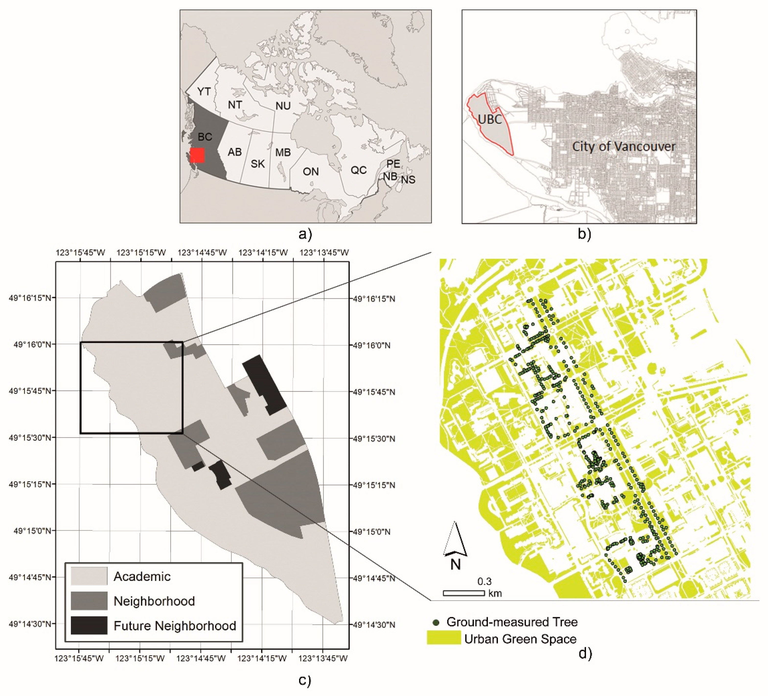
Figure 1. (a) Provinces of Canada; (b) geographical location of study area (University of British Columbia (UBC) Point Grey campus); (c) land use of UBC; (d) the specific survey area.
Forests 12 00062 g001
Figure 2. Section of light detection and ranging (LiDAR) data colored by height on the Vancouver UBC main campus (generated in LiDAR360 v4.0 by GreenValley International).
Forests 12 00062 g002
Figure 3. Methodological framework (generated in LiDAR360 v4.0 by GreenValley International and R-lidR package).
Forests 12 00062 g003
Figure 4. Steps and processes for AITD (AITD: automated individual tree detection, CHM: canopy height model).
Forests 12 00062 g004
Figure 5. (A) Errors of commission: tree crowns are segmented into multiple segments; (B) errors of omission: multiple tree crowns are delineated by a single segment. X represents a tree trunk (confirmed in the field, i.e., ground-truthed).
Forests 12 00062 g005
Figure 6. Workflow for DBH and carbon modeling (CA: canopy area, MTH: measured tree height, TH: LiDAR tree height, CW: canopy width, DBH: diameter outside bark at breast height, th: threshold, AIC: Akaike’s information criterion).
Forests 12 00062 g006
Figure 7. Individual trees depend on different AITD routines: (a) marker-controlled watershed segmentation; (b) simple watershed segmentation; (c) AITD by Dalponte and Coomes [68]; (d) AITD by Silva et al. [69]; (e) AITD by Li et al. [56].
Forests 12 00062 g007
Figure 8. Kernel density and carbon storage map of the UBC campus in Vancouver, using results from the estimation model.
Forests 12 00062 g008
Table 1. Results of AITD accuracy for 300 individual trees (MT: the number of matched trees, OE: the number of omission errors, CE: the number of commission errors, Re: recall, Pr: precision, F: F-score).
AITDMTOECERePrF
Marker controlled watershed segmentation32542180.890.950.92
Simple watershed segmentation3207580.980.850.91
Dalponte and Coomes (2016)3637150.980.960.97
Silva et al. (2016)30350320.860.900.88
Li et al. (2012)28769290.810.910.85
Table 2. AIC, log-likelihood, and RMSE values according to the nls model (AIC: Akaike’s information criterion, Log-Lik: log-likelihood, RMSE: root-mean-squared error).
Parameternls Model
Max_crAICLog-LikRMSE
103210.82−1601.4119.69
153242.20−1617.1019.83
203196.88−1594.4419.55
253228.22−1610.1119.69
303228.22−1610.1119.63
Publisher’s Note: MDPI stays neutral with regard to jurisdictional claims in published maps and institutional affiliations.