Monitoring Mangrove Forest Degradation and Regeneration: Landsat Time Series Analysis of Moisture and Vegetation Indices at Rabigh Lagoon, Red Sea


Abstract
1. Introduction
2. Materials and Methods
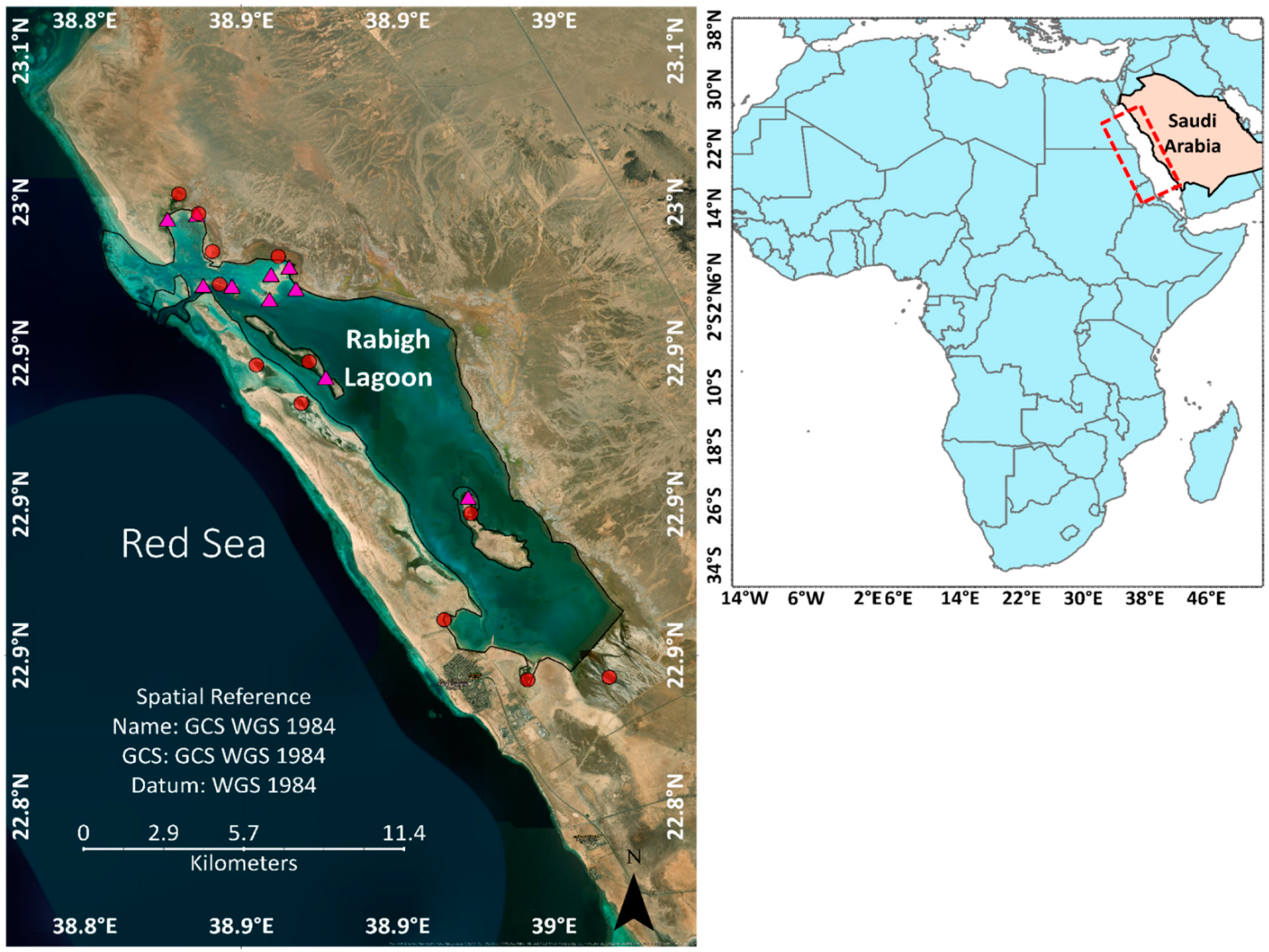
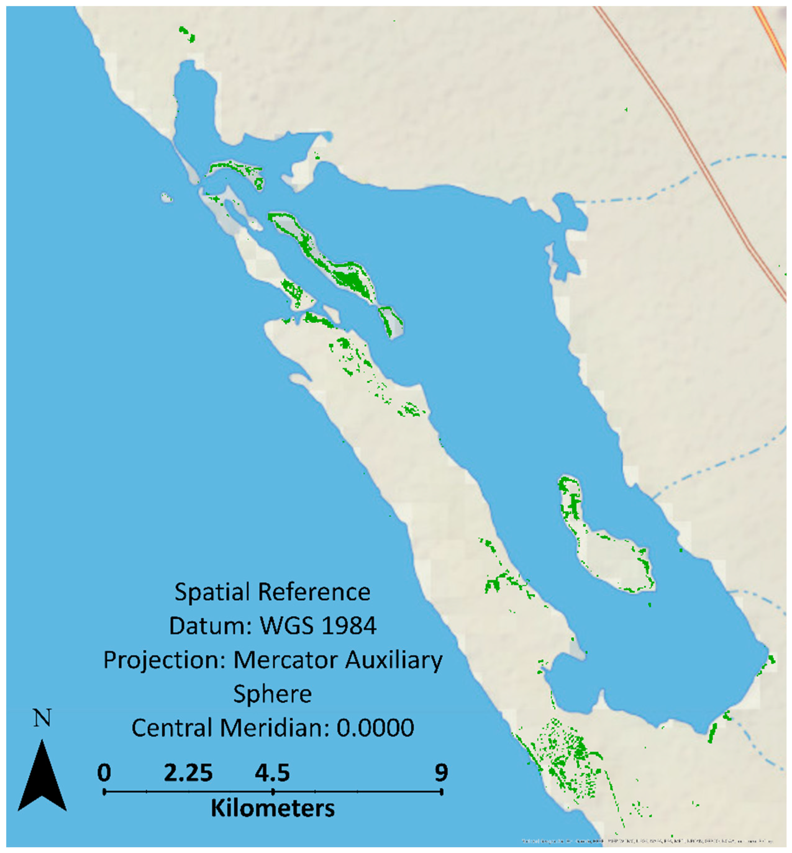
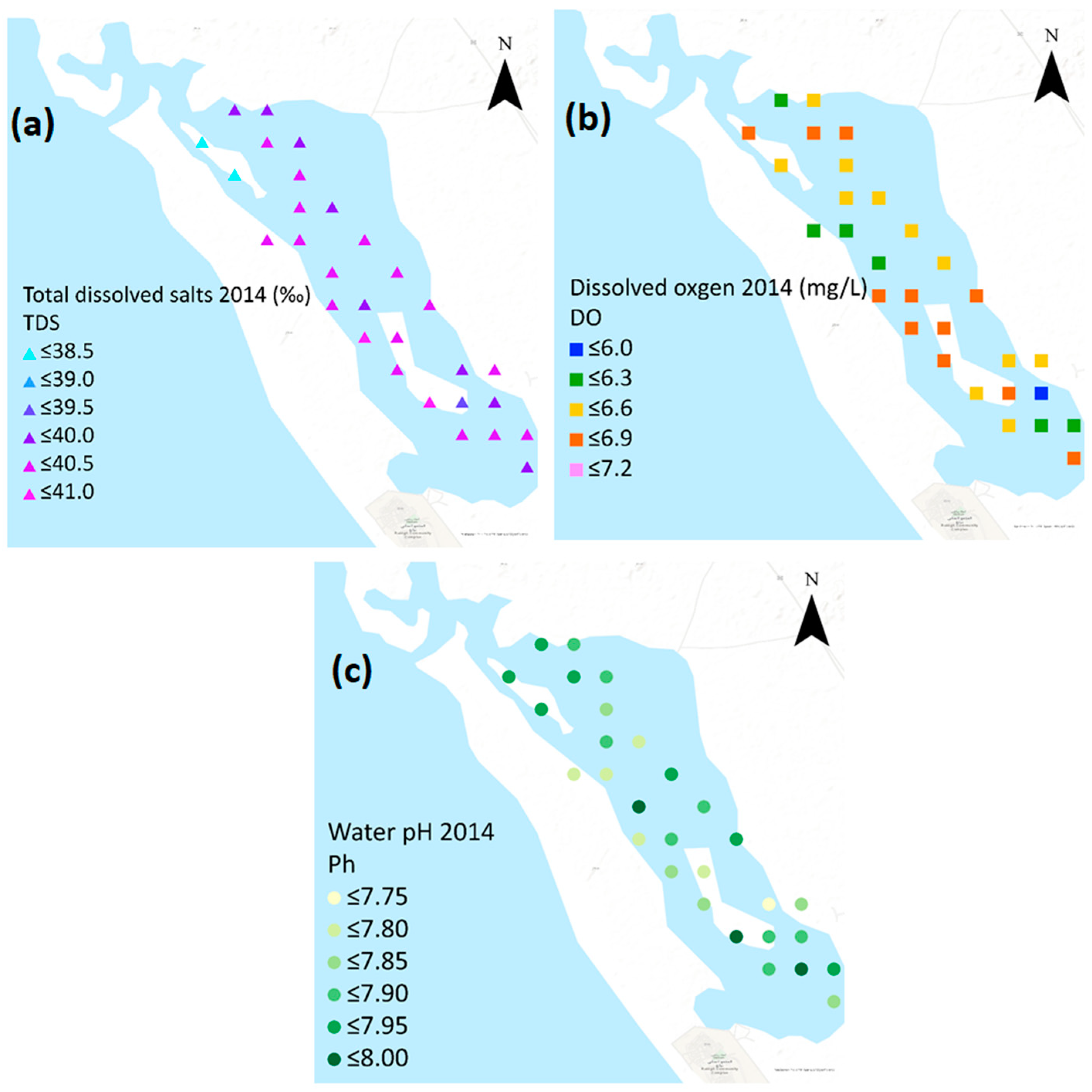
2.1. Study Area
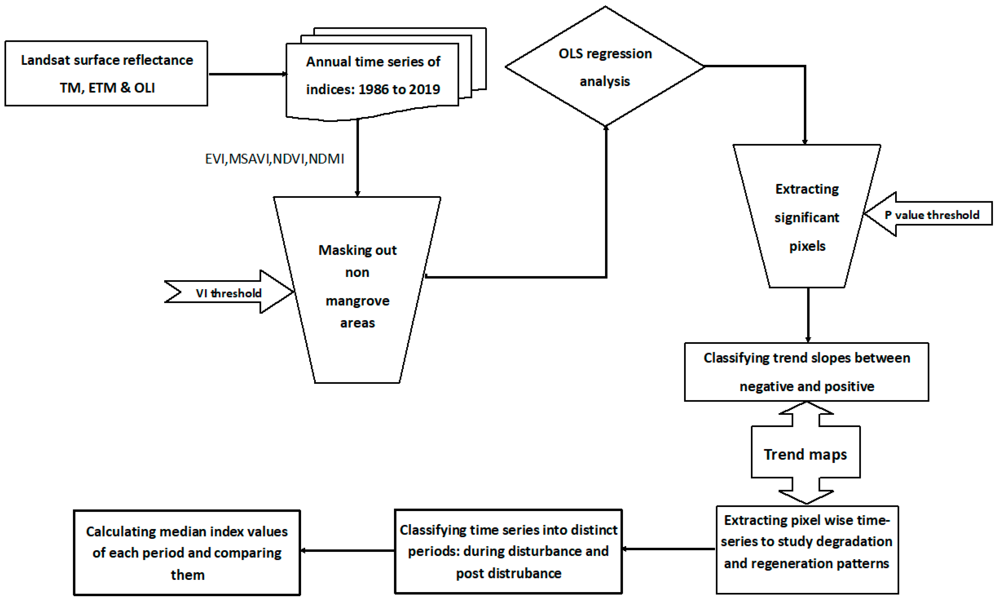
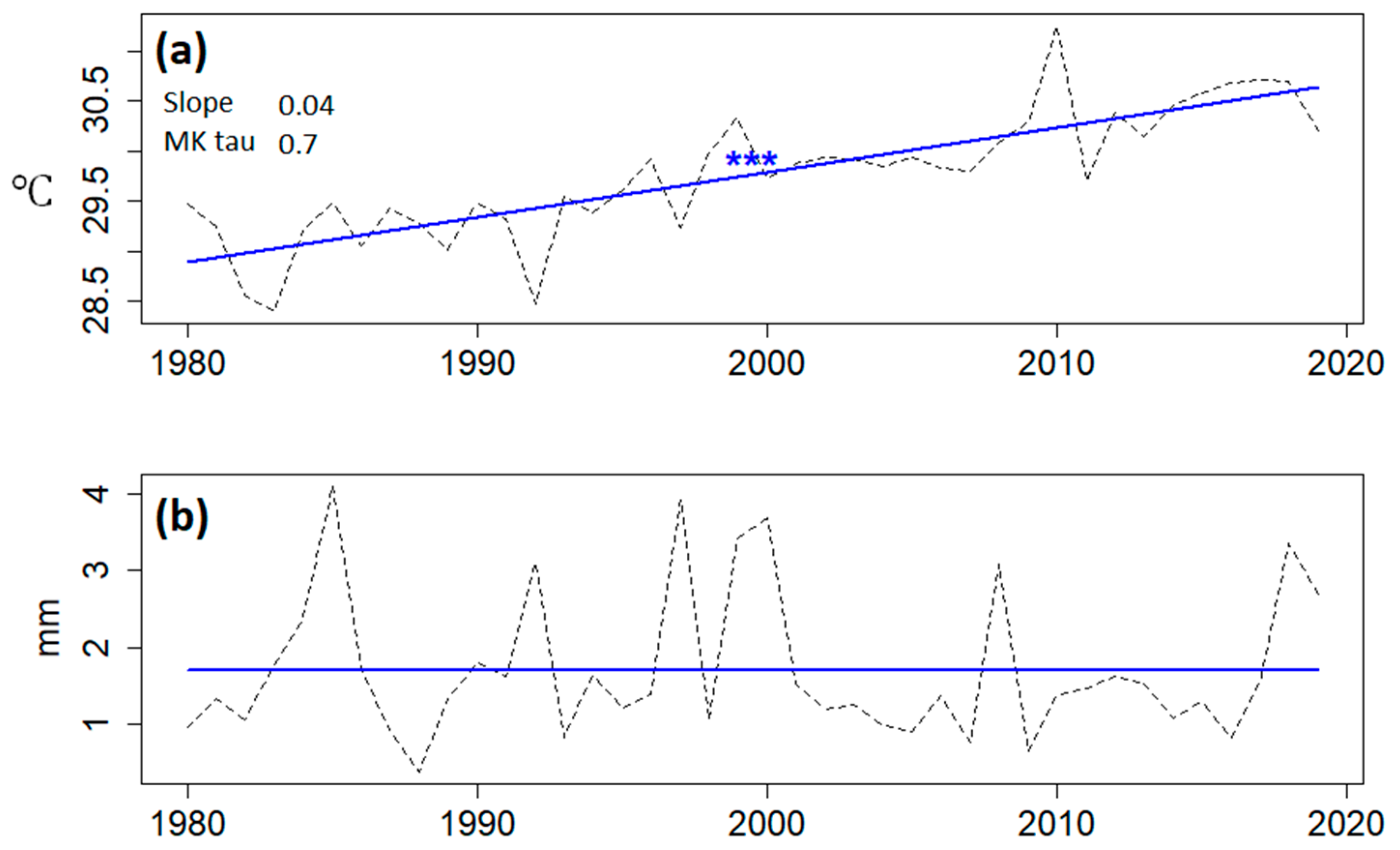
2.2. Trend Analysis Using Time Series
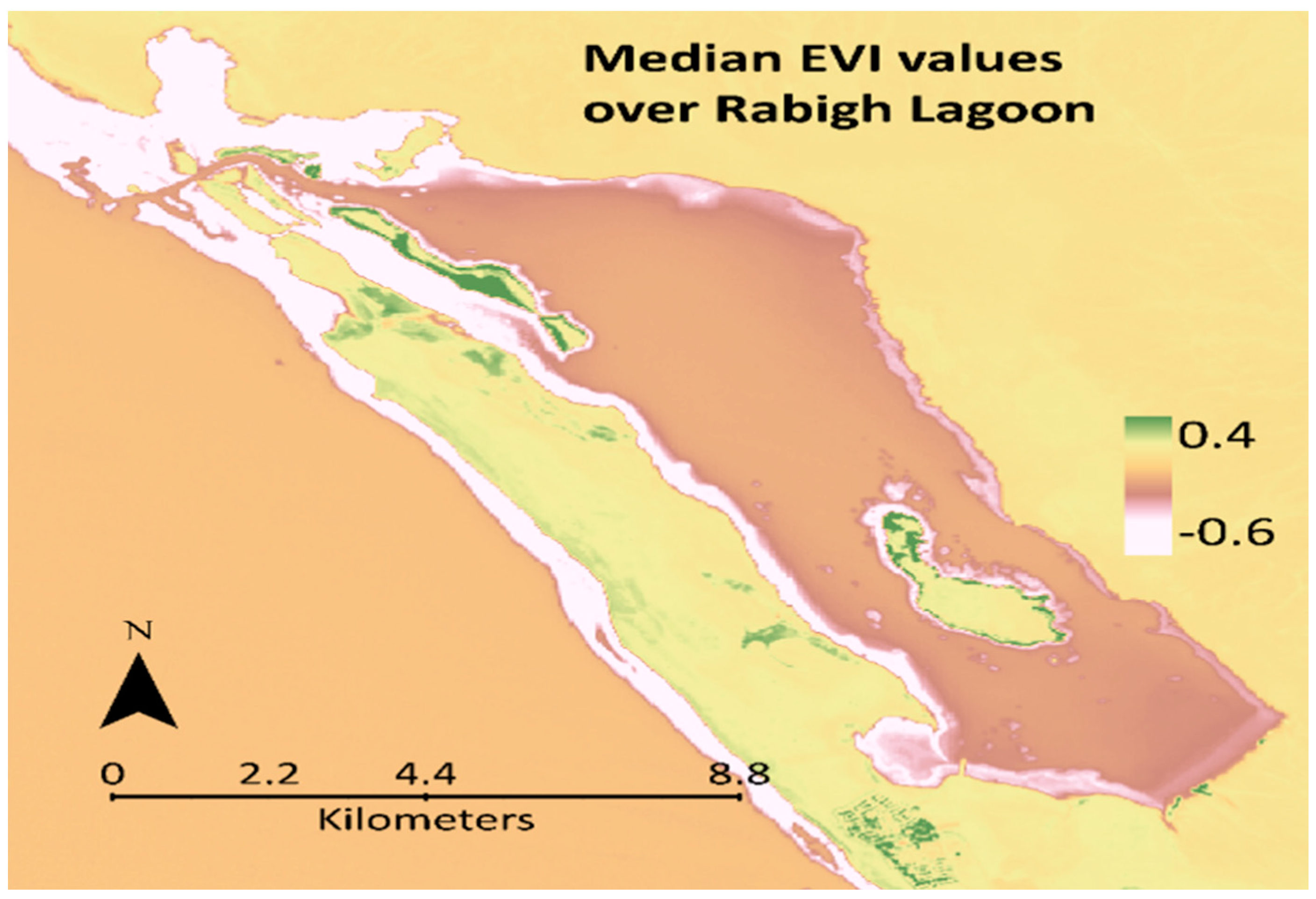
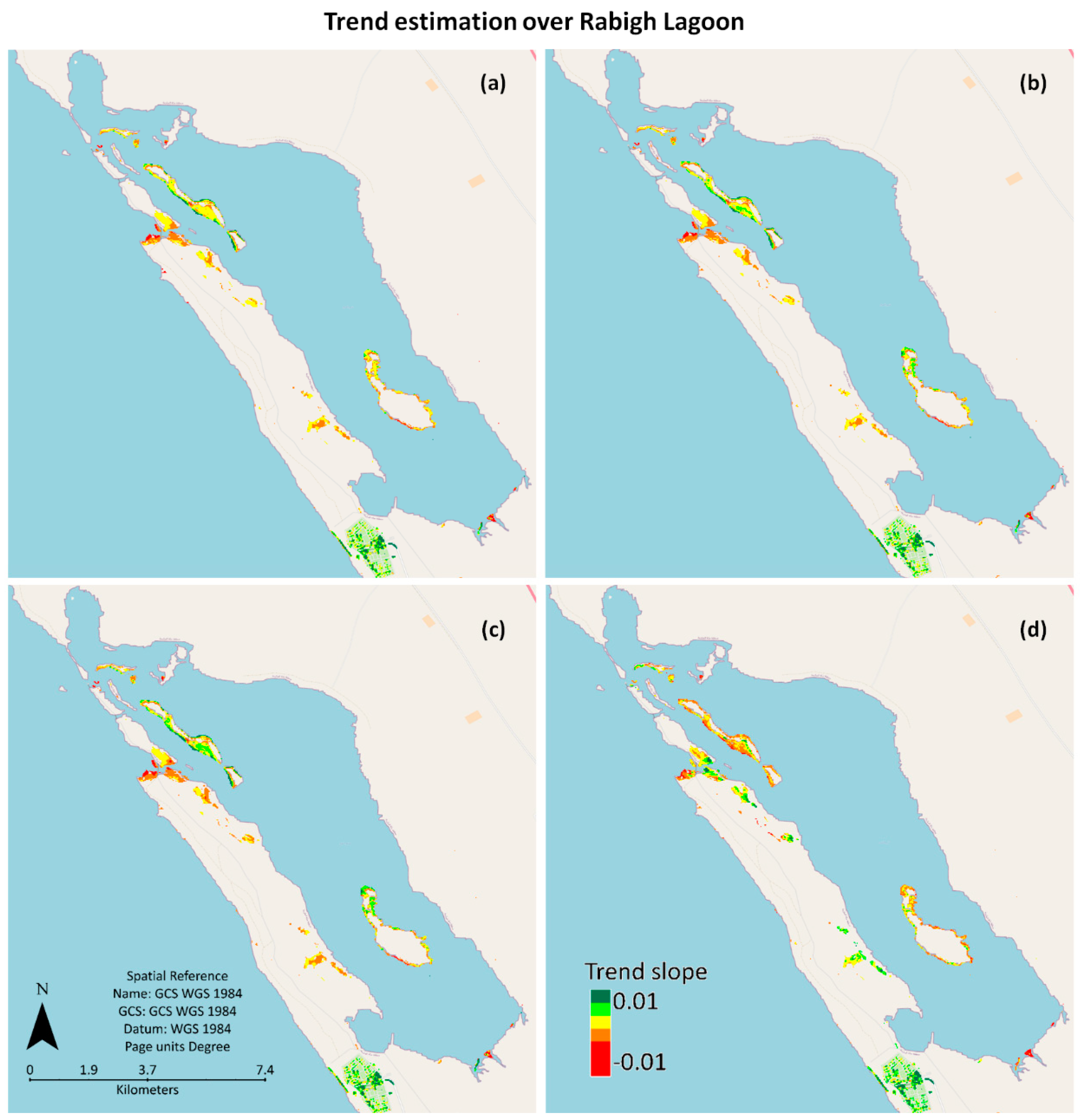
3. Results
4. Discussion
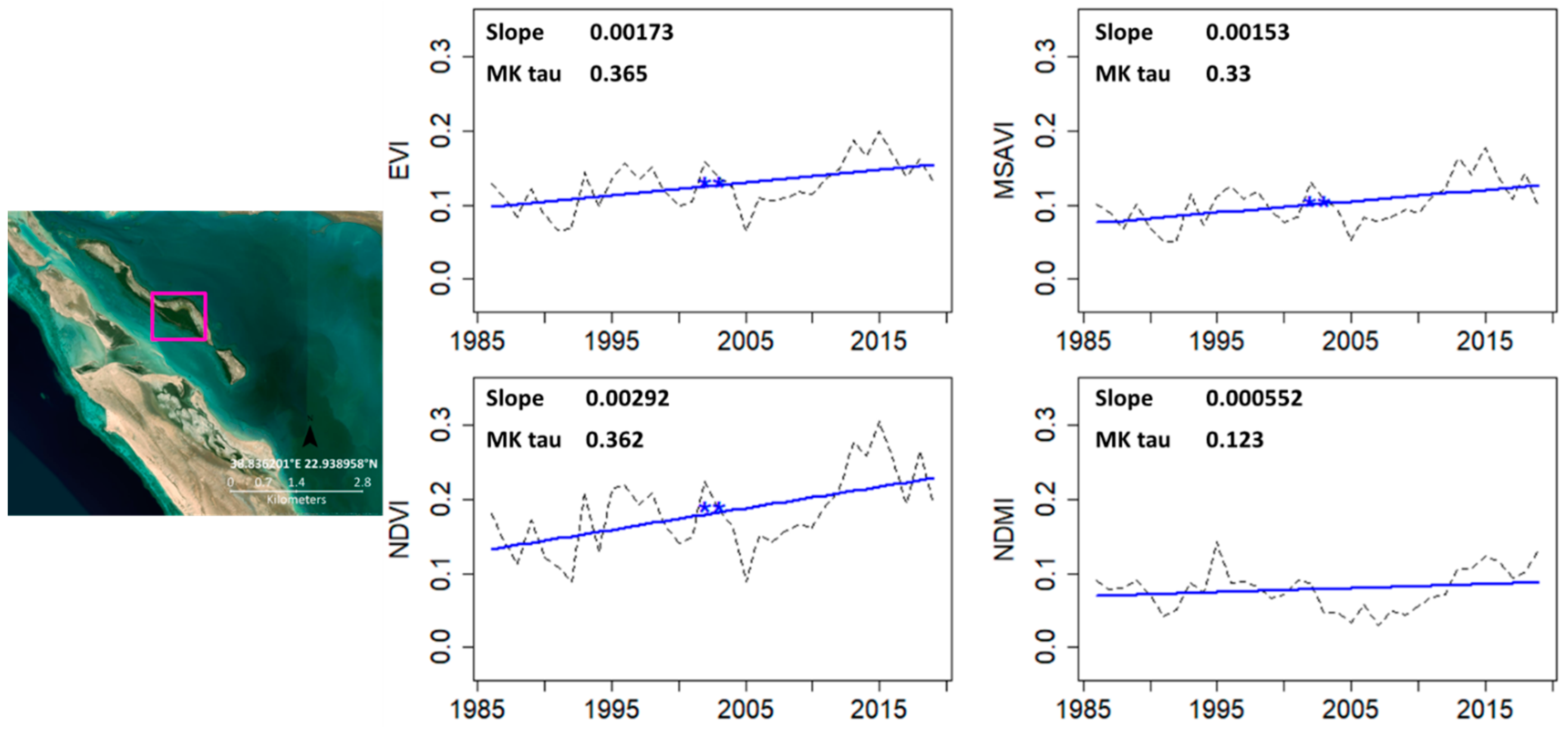
4.1. North of Lagoon
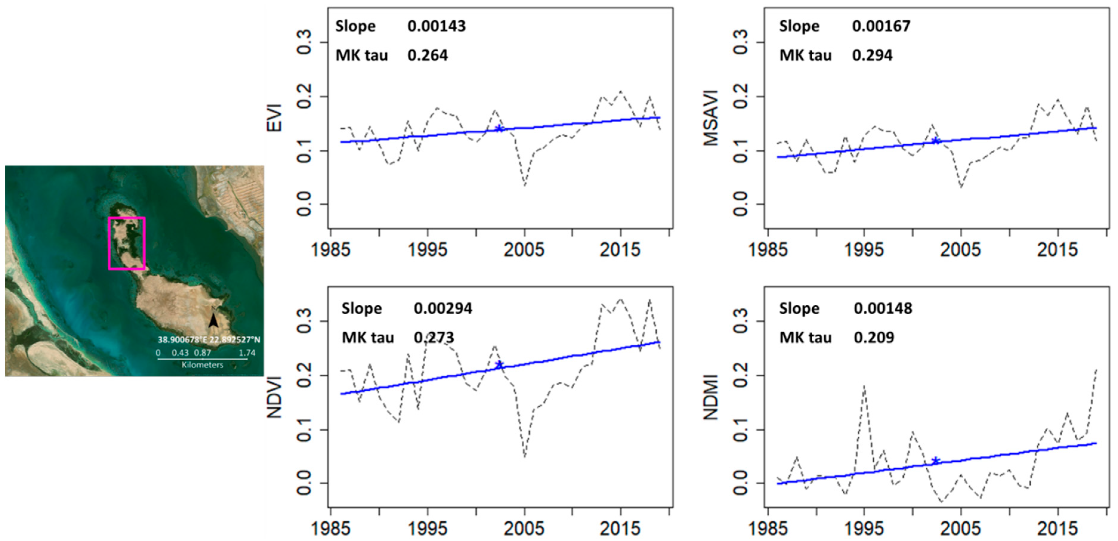
4.2. South of Lagoon
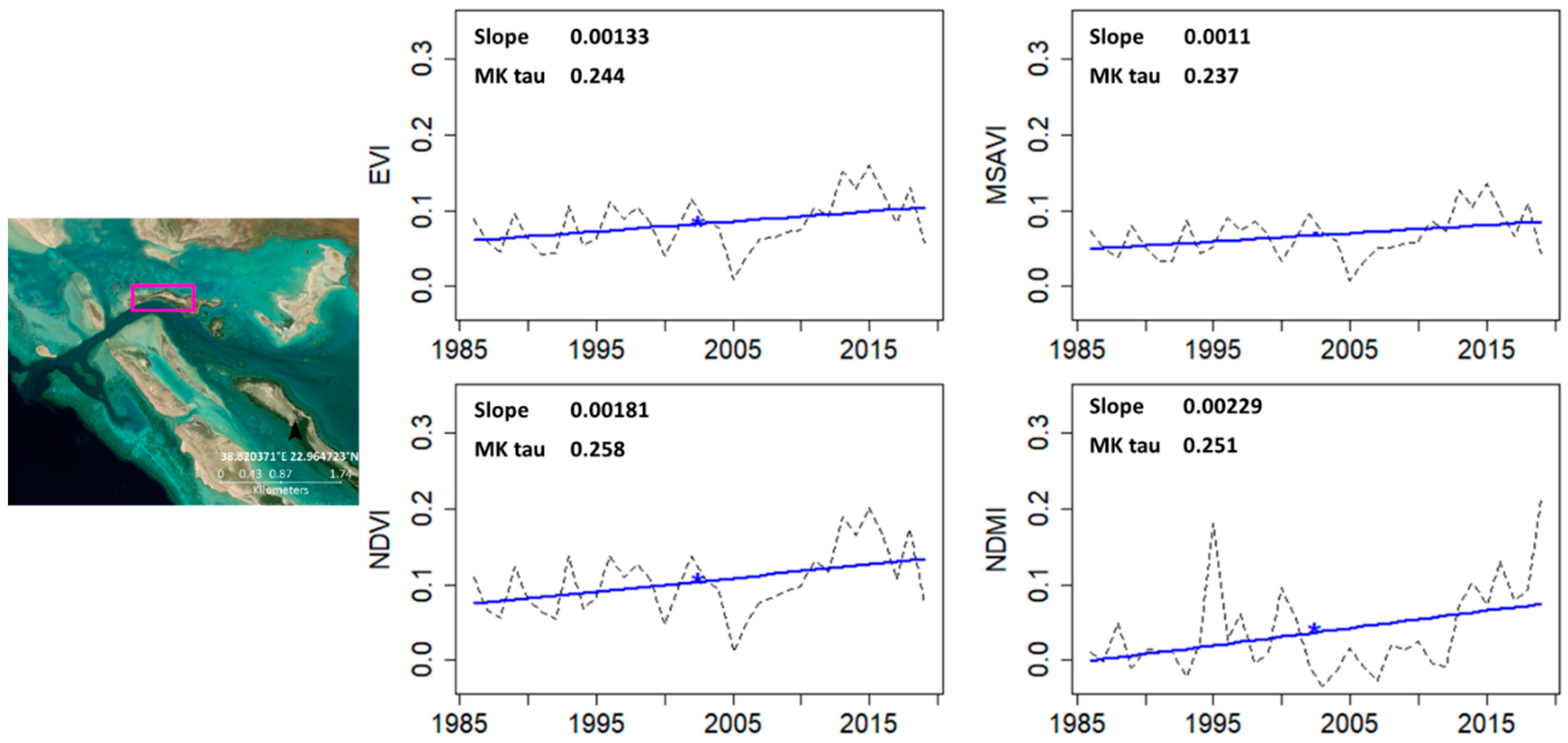
4.3. Extreme Northwest of Lagoon
5. Conclusions
Author Contributions
Funding
Acknowledgments
Conflicts of Interest
References
- Guangyi, Z. Influences of tropical forest changes on environmental quality in Hainan province, PR of China. Ecol. Eng. 1995, 4, 223–229. [Google Scholar] [CrossRef]
- Costanza, R.; d’Arge, R.; De Groot, R.; Farber, S.; Grasso, M.; Hannon, B.; Limburg, K.; Naeem, S.; O’neill, R.V.; Paruelo, J. The value of the world’s ecosystem services and natural capital. Nature 1997, 387, 253–260. [Google Scholar] [CrossRef]
- Khan, W.R.; Nazre, M.; Zulkifli, S.Z.; Kudus, K.A.; Zimmer, M.; Roslan, M.K.; Mukhtar, A.; Mostapa, R.; Gandaseca, S. Reflection of stable isotopes and selected elements with the inundation gradient at the Matang Mangrove Forest Reserve (MMFR), Malaysia. Int. For. Rev. 2017, 19, 1–10. [Google Scholar] [CrossRef]
- Lee, H.-Y.; Shih, S.-S. Impacts of vegetation changes on the hydraulic and sediment transport characteristics in Guandu mangrove wetland. Ecol. Eng. 2004, 23, 85–94. [Google Scholar] [CrossRef]
- Lewis, R.R., III. Ecological engineering for successful management and restoration of mangrove forests. Ecol. Eng. 2005, 24, 403–418. [Google Scholar] [CrossRef]
- Willis, J.M.; Hester, M.W.; Shaffer, G.P. A mesocosm evaluation of processed drill cuttings for wetland restoration. Ecol. Eng. 2005, 25, 41–50. [Google Scholar] [CrossRef]
- Sánchez-Carrillo, S.; Sánchez-Andrés, R.; Alatorre, L.C.; Angeler, D.G.; Álvarez-Cobelas, M.; Arreola-Lizárraga, J.A. Nutrient fluxes in a semi-arid microtidal mangrove wetland in the Gulf of California. Estuar. Coast. Shelf Sci. 2009, 82, 654–662. [Google Scholar] [CrossRef]
- Fickert, T. To Plant or Not to Plant, That Is the Question: Reforestation vs. Natural Regeneration of Hurricane-Disturbed Mangrove Forests in Guanaja (Honduras). Forests 2020, 11, 1068. [Google Scholar] [CrossRef]
- Khan, W.R.; Rasheed, F.; Zulkifli, S.Z.; Kasim, M.R.B.M.; Zimmer, M.; Pazi, A.M.; Kamrudin, N.A.; Zafar, Z.; Faridah-Hanum, I.; Nazre, M. Phytoextraction Potential of Rhizophora Apiculata: A Case Study in Matang Mangrove Forest Reserve, Malaysia. Trop. Conserv. Sci. 2020, 13, 1940082920947344. [Google Scholar] [CrossRef]
- Kathiresan, K.; Bingham, B.L. Biology of mangroves and mangrove ecosystems. Adv. Mar. Biol. 2001, 40, 84–254. [Google Scholar]
- Spalding, M.; Blasco, F.; Field, C. World Mangrove Atlas; International Society for Mangrove Ecosystems: Okinawa, Japan, 1997; Available online: www.environmentalunit.com/Documentation/04%20Resources%20at%20Risk/World%20mangrove%20atlas.pdf (accessed on 15 October 2020).
- Dahdouh-Guebas, F.; Mathenge, C.; Kairo, J.G.; Koedam, N. Utilization of mangrove wood products around Mida Creek (Kenya) amongst subsistence and commercial users. Econ. Bot. 2000, 54, 513–527. [Google Scholar] [CrossRef]
- Ruiz-Luna, A.; Berlanga-Robles, C.A. Land use, land cover changes and coastal lagoon surface reduction associated with urban growth in northwest Mexico. Landsc. Ecol. 2003, 18, 159–171. [Google Scholar] [CrossRef]
- Ruiz-Luna, A.; Acosta-Velázquez, J.; Berlanga-Robles, C.A. On the reliability of the data of the extent of mangroves: A case study in Mexico. Ocean Coast. Manag. 2008, 51, 342–351. [Google Scholar] [CrossRef]
- Saenger, P.; Khalil, A.S.M. Regional Action Plan for the Conservation of Mangroves. In PERGA/GEF Regional Action Plan for the Conservation of Marine Turtles, Seabirds and Mangroves in the Red Sea and Gulf of Aden; Technical Series 12; PERSGA: Jeddah, Saudi Arabia, 2007; pp. 101–129. [Google Scholar]
- Khalil, A.S.M.; Krupp, F. Fishes of the mangrove ecosystem. In Comparative Ecological Analysis of Biota and Habitats in Littoral and Shallow Sublittoral Waters of the Sudanese Red Sea; Report for the Period of Apr 1991–Dec 1993; Faculty of Marine Science and Fisheries, Port Sudan, and ForschungsinstitutSenckenberg: Frankfurt, Germany, 1994. [Google Scholar]
- Wilkie, M.L. Mangrove Conservation and Management in the Sudan; Consultancy Report. Based on the Work of Ministry of Environment and Tourism. FOL/CF Sudan. FP:GCP/SUD/O47/NET; FAO: Khartoum, Sudan, 1995; 92p. [Google Scholar]
- Ormond, R.F.G. Management and conservation of Red Sea habitats. In The coastal and marine environments of the Red Sea, Gulf of Aden and Tropical Western Indian Ocean. Proceedings of Symposium, Khartoum (January). The Red Sea and the Gulf of Aden Environmental Programme Jeddah; 1980; Volume 2, pp. 135–162. Available online: http://www.reefbase.org/resource_center/publication/pub_4287.aspx (accessed on 15 October 2020).
- Mandura, A.S. A mangrove stand under sewage pollution stress: Red Sea. Mangroves Salt Marshes 1997, 1, 255–262. [Google Scholar] [CrossRef]
- Raitsos, D.E.; Hoteit, I.; Prihartato, P.K.; Chronis, T.; Triantafyllou, G.; Abualnaja, Y. Abrupt warming of the Red Sea. Geophys. Res. Lett. 2011, 38. [Google Scholar] [CrossRef]
- Rasolofoharinoro, M.; Blasco, F.; Bellan, M.F.; Aizpuru, M.; Gauquelin, T.; Denis, J. A remote sensing based methodology for mangrove studies in Madagascar. Int. J. Remote Sens. 1998, 19, 1873–1886. [Google Scholar] [CrossRef]
- Gao, J. A comparative study on spatial and spectral resolutions of satellite data in mapping mangrove forests. Int. J. Remote Sens. 1999, 20, 2823–2833. [Google Scholar] [CrossRef]
- Blasco, F.; Aizpuru, M. Mangroves along the coastal stretch of the Bay of Bengal: Present status. Ind. J. Mar. Sci. 2002, 31, 9–20. [Google Scholar]
- Saito, H.; Bellan, M.F.; Al-Habshi, A.; Aizpuru, M.; Blasco, F. Mangrove research and coastal ecosystem studies with SPOT-4 HRVIR and TERRA ASTER in the Arabian Gulf. Int. J. Remote Sens. 2003, 24, 4073–4092. [Google Scholar] [CrossRef]
- Alatorre, L.C.; Sánchez-Andrés, R.; Cirujano, S.; Beguería, S.; Sánchez-Carrillo, S. Identification of mangrove areas by remote sensing: The ROC curve technique applied to the northwestern Mexico coastal zone using Landsat imagery. Remote Sens. 2011, 3, 1568–1583. [Google Scholar] [CrossRef]
- Jensen, J.R.; Lin, H.; Yang, X.; Ramsey, E., III; Davis, B.A.; Thoemke, C.W. The measurement of mangrove characteristics in southwest Florida using SPOT multispectral data. Geocarto Int. 1991, 6, 13–21. [Google Scholar] [CrossRef]
- Ramsey, E.W., III; Jensen, J.R. Remote sensing of mangrove wetlands: Relating canopy spectra to site-specific data. Photogramm. Eng. Remote Sens. 1996, 62, 939–948. [Google Scholar]
- Green, E.P.; Mumby, P.J.; Edwards, A.J.; Clark, C.D.; Ellis, A.C. Estimating leaf area index of mangroves from satellite data. Aquat. Bot. 1997, 58, 11–19. [Google Scholar] [CrossRef]
- Green, E.P.; Clark, C.D.; Mumby, P.J.; Edwards, A.J.; Ellis, A.C. Remote sensing techniques for mangrove mapping. Int. J. Remote Sens. 1998, 19, 935–956. [Google Scholar] [CrossRef]
- Green, E.; Mumby, P.; Edwards, A.; Clark, C. Remote Sensing: Handbook for Tropical Coastal Management; United Nations Educational, Scientific and Cultural Organization (UNESCO): Paris, France, 2000. [Google Scholar]
- Huete, A.; Didan, K.; Miura, T.; Rodriguez, E.P.; Gao, X.; Ferreira, L.G. Overview of the radiometric and biophysical performance of the MODIS vegetation indices. Remote Sens. Environ. 2002, 83, 195–213. [Google Scholar] [CrossRef]
- Gao, B.-C. NDWI—A normalized difference water index for remote sensing of vegetation liquid water from space. Remote Sens. Environ. 1996, 58, 257–266. [Google Scholar] [CrossRef]
- Almahasheer, H.; Aljowair, A.; Duarte, C.M.; Irigoien, X. Decadal stability of Red Sea mangroves. Estuar. Coast. Shelf Sci. 2016, 169, 164–172. [Google Scholar] [CrossRef]
- Elsebaie, I.H.; Aguib, A.S.H.; Al Garni, D. The Role of Remote Sensing and GIS for Locating Suitable Mangrove Plantation Sites Along the Southern Saudi Arabian Red Sea. Int. J. Geosci. 2013, 4, 471–479. [Google Scholar] [CrossRef]
- Kumar, A.; Khan, M.A.; Muqtadir, A. Distribution of mangroves along the Red Sea coast of the Arabian Peninsula: Part-I: The northern coast of western Saudi Arabia. Earth Sci. India 2010, 3. [Google Scholar]
- Abd-El Monsef, H.; Smith, S.E. A new approach for estimating mangrove canopy cover using Landsat 8 imagery. Comput. Electron. Agric. 2017, 135, 183–194. [Google Scholar] [CrossRef]
- Braithwaite, C.J.R. Geology and Palaeogeography of the Red Sea Region; Edwards, A.J., Head, S.M., Eds.; Red Sea (Key Environments); Pergamon Press: Oxford, UK, 1987; pp. 22–44. [Google Scholar]
- Brown, G.F.; Schmidt, D.L.; Huffman, A.C., Jr. Geology of the Arabian Peninsula; Shield Area of Western Saudi Arabia (No. 560-A); US Geological Survey: Reston, VA, USA, 1989; 188p.
- Al-Washmi, H.A. Sedimentological aspects and environmental conditions recognized from the bottom sediments of Al-Kharrar Lagoon, eastern Red Sea coastal plain, Saudi Arabia. J. KAU Mar. Sci 1999, 10, 71–87. [Google Scholar] [CrossRef]
- Al-Dubai, T.A.; Abu-Zied, R.H.; Basaham, A.S. Present environmental status of Al-Kharrar Lagoon, central of the eastern Red Sea coast, Saudi Arabia. Arab. J. Geosci. 2017, 10, 305. [Google Scholar] [CrossRef]
- Aljahdali, M.O.; Alhassan, A.B. Ecological risk assessment of heavy metal contamination in mangrove habitats, using biochemical markers and pollution indices: A case study of Avicennia marina L. in the Rabigh lagoon, Red Sea. Saudi J. Biol. Sci. 2020, 27, 1174–1184. [Google Scholar] [CrossRef] [PubMed]
- Bahrawi, J.A.; Elhag, M.; Aldhebiani, A.Y.; Galal, H.K.; Hegazy, A.K.; Alghailani, E. Soil erosion estimation using remote sensing techniques in Wadi Yalamlam Basin, Saudi Arabia. Adv. Mater. Sci. Eng. 2016, 2016, 1–8. [Google Scholar] [CrossRef]
- Schmidt, G.L.; Jenkerson, C.B.; Masek, J.; Vermote, E.; Gao, F. Landsat Ecosystem Disturbance Adaptive Processing System (LEDAPS) Algorithm Description. Available online: https://pubs.er.usgs.gov/publication/ofr20131057 (accessed on 17 March 2015).
- Vermote, E.; Justice, C.; Claverie, M.; Franch, B. Preliminary analysis of the performance of the Landsat 8/OLI land surface reflectance product. Remote Sens. Environ. 2016, 185, 46–56. [Google Scholar] [CrossRef]
- Wilson, E.H.; Sader, S.A. Detection of forest harvest type using multiple dates of Landsat TM imagery. Remote Sens. Environ. 2002, 80, 385–396. [Google Scholar] [CrossRef]
- Qi, J.; Chehbouni, A.; Huete, A.R.; Kerr, Y.H.; Sorooshian, S. A modified soil adjusted vegetation index. Remote Sens. Environ. 1994, 48, 119–126. [Google Scholar] [CrossRef]
- Fensholt, R.; Horion, S.; Tagesson, T.; Ehammer, A.; Grogan, K.; Tian, F.; Huber, S.; Verbesselt, J.; Prince, S.D.; Tucker, C.J. Assessment of vegetation trends in drylands from time series of earth observation data. In Remote Sensing Time Series; Springer: Berlin/Heidelberg, Germany, 2015; pp. 159–182. [Google Scholar]
- Ollinger, S.V. Sources of variability in canopy reflectance and the convergent properties of plants. New Phytol. 2011, 189, 375–394. [Google Scholar] [CrossRef]
- Forkel, M.; Carvalhais, N.; Verbesselt, J.; Mahecha, M.D.; Neigh, C.S.R.; Reichstein, M. Trend change detection in NDVI time series: Effects of inter-annual variability and methodology. Remote Sens. 2013, 5, 2113–2144. [Google Scholar] [CrossRef]
- Zeileis, A.; Shah, A.; Patnaik, I. Testing, monitoring, and dating structural changes in exchange rate regimes. Comput. Stat. Data Anal. 2010, 54, 1696–1706. [Google Scholar] [CrossRef]
- Bai, J.; Perron, P. Computation and analysis of multiple structural change models. J. Appl. Econom. 2003, 18, 1–22. [Google Scholar] [CrossRef]
- Jin, S.; Sader, S.A. Comparison of time series tasseled cap wetness and the normalized difference moisture index in detecting forest disturbances. Remote Sens. Environ. 2005, 94, 364–372. [Google Scholar] [CrossRef]
- Lugo, A.E.; Snedaker, S.C. The ecology of mangroves. Annu. Rev. Ecol. Syst. 1974, 5, 39–64. [Google Scholar] [CrossRef]
- Youssef, M.; El-Sorogy, A. Environmental assessment of heavy metal contamination in bottom sediments of Al-Kharrar lagoon, Rabigh, Red Sea, Saudi Arabia. Arab. J. Geosci. 2016, 9, 474. [Google Scholar] [CrossRef]
- Yahiya, A.B. Environmental degradation and its impact on tourism in Jazan, KSA using remote sensing and GIS. Int. J. Environ. Sci. 2012, 3, 421–432. [Google Scholar]
- Mayr, S.; Kuenzer, C.; Gessner, U.; Klein, I.; Rutzinger, M. Validation of Earth Observation Time-Series: A Review for Large-Area and Temporally Dense Land Surface Products. Remote Sens. 2019, 11, 2616. [Google Scholar] [CrossRef]
- Krishnamurthy, P.; Mohanty, B.; Wijaya, E.; Lee, D.-Y.; Lim, T.-M.; Lin, Q.; Xu, J.; Loh, C.-S.; Kumar, P.P. Transcriptomics analysis of salt stress tolerance in the roots of the mangrove Avicennia officinalis. Sci. Rep. 2017, 7, 1–19. [Google Scholar] [CrossRef]
- Vovides, A.G.; López-Portillo, J.; Bashan, Y. N 2-fixation along a gradient of long-term disturbance in tropical mangroves bordering the Gulf of Mexico. Biol. Fertil. Soils 2011, 47, 567–576. [Google Scholar] [CrossRef]
- Twilley, R.R.; Rivera-Monroy, V.H.; Chen, R.; Botero, L. Adapting an ecological mangrove model to simulate trajectories in restoration ecology. Mar. Pollut. Bull. 1999, 37, 404–419. [Google Scholar] [CrossRef]
- Reef, R.; Lovelock, C.E. Regulation of water balance in mangroves. Ann. Bot. 2015, 115, 385–395. [Google Scholar] [CrossRef]


| Spectral Index | Formula | Wavelength (µm) | Reference | |
|---|---|---|---|---|
| NDVI | (NIR − Red)/(NIR + Red) | Red | 0.63–0.69 | [45] |
| EVI | G * (NIR − Red)/(NIR + C1 * Red − C2 * Blue + L) | Blue | 0.45–0.52 | [46] |
| MSAVI | (2 * NIR + 1 − sqrt ((2 * NIR + 1)2 − 8 * (NIR − Red))/2 | NIR(near infrared) | 0.77–0.9 | [47] |
| NDMI | (NIR − SWIR1)/(NIR + SWIR1) | SWIR1(shortwave infrared) | 1.55–1.75 | [31] |
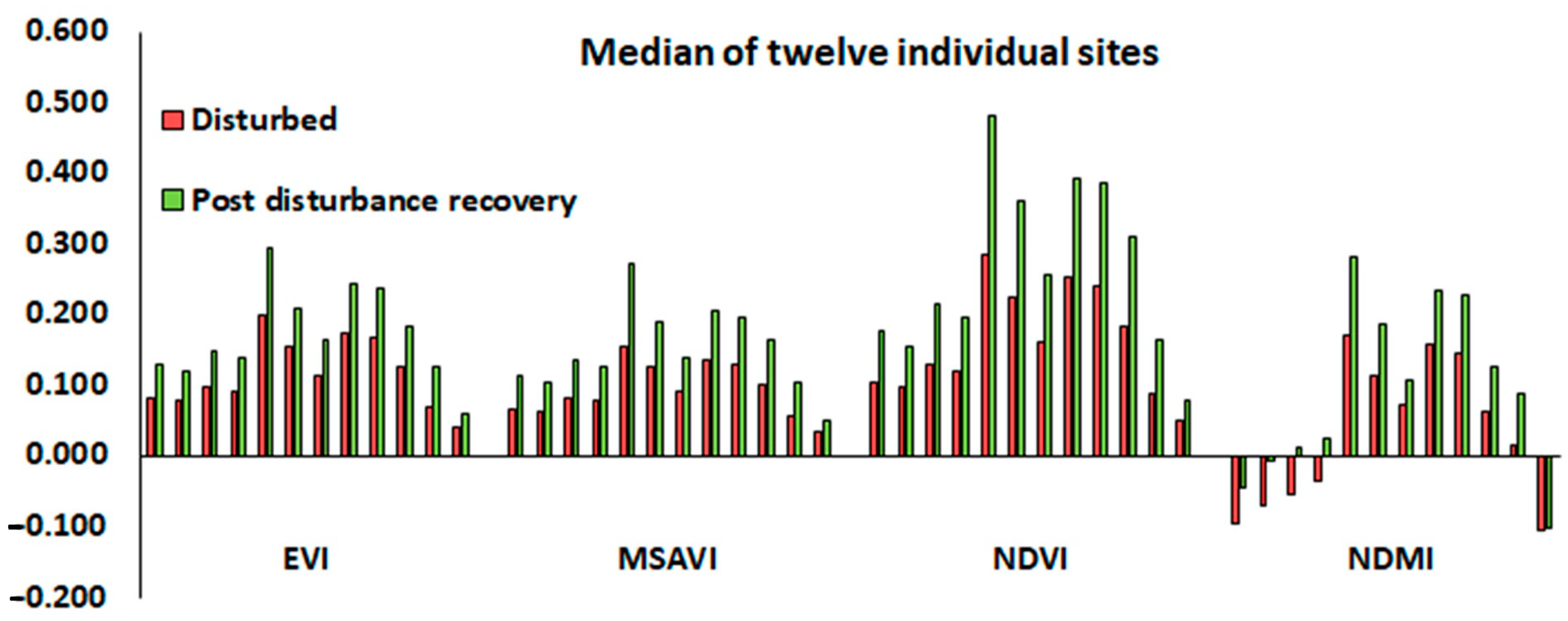
| Index | Disturbance | Recovery | Difference |
|---|---|---|---|
| EVI | 0.104 | 0.155 | 0.052 |
| MSAVI | 0.086 | 0.136 | 0.051 |
| NDVI | 0.143 | 0.235 | 0.092 |
| NDMI | 0.038 | 0.096 | 0.066 |
Publisher’s Note: MDPI stays neutral with regard to jurisdictional claims in published maps and institutional affiliations. |
© 2021 by the authors. Licensee MDPI, Basel, Switzerland. This article is an open access article distributed under the terms and conditions of the Creative Commons Attribution (CC BY) license (http://creativecommons.org/licenses/by/4.0/).
Share and Cite
Aljahdali, M.O.; Munawar, S.; Khan, W.R. Monitoring Mangrove Forest Degradation and Regeneration: Landsat Time Series Analysis of Moisture and Vegetation Indices at Rabigh Lagoon, Red Sea. Forests 2021, 12, 52. https://doi.org/10.3390/f12010052
Aljahdali MO, Munawar S, Khan WR. Monitoring Mangrove Forest Degradation and Regeneration: Landsat Time Series Analysis of Moisture and Vegetation Indices at Rabigh Lagoon, Red Sea. Forests. 2021; 12(1):52. https://doi.org/10.3390/f12010052
Chicago/Turabian StyleAljahdali, Mohammed Othman, Sana Munawar, and Waseem Razzaq Khan. 2021. "Monitoring Mangrove Forest Degradation and Regeneration: Landsat Time Series Analysis of Moisture and Vegetation Indices at Rabigh Lagoon, Red Sea" Forests 12, no. 1: 52. https://doi.org/10.3390/f12010052
APA StyleAljahdali, M. O., Munawar, S., & Khan, W. R. (2021). Monitoring Mangrove Forest Degradation and Regeneration: Landsat Time Series Analysis of Moisture and Vegetation Indices at Rabigh Lagoon, Red Sea. Forests, 12(1), 52. https://doi.org/10.3390/f12010052