Assessment of Sentinel-2 Satellite Images and Random Forest Classifier for Rainforest Mapping in Gabon

 ,
,  ,
,  and
and
Abstract
1. Introduction
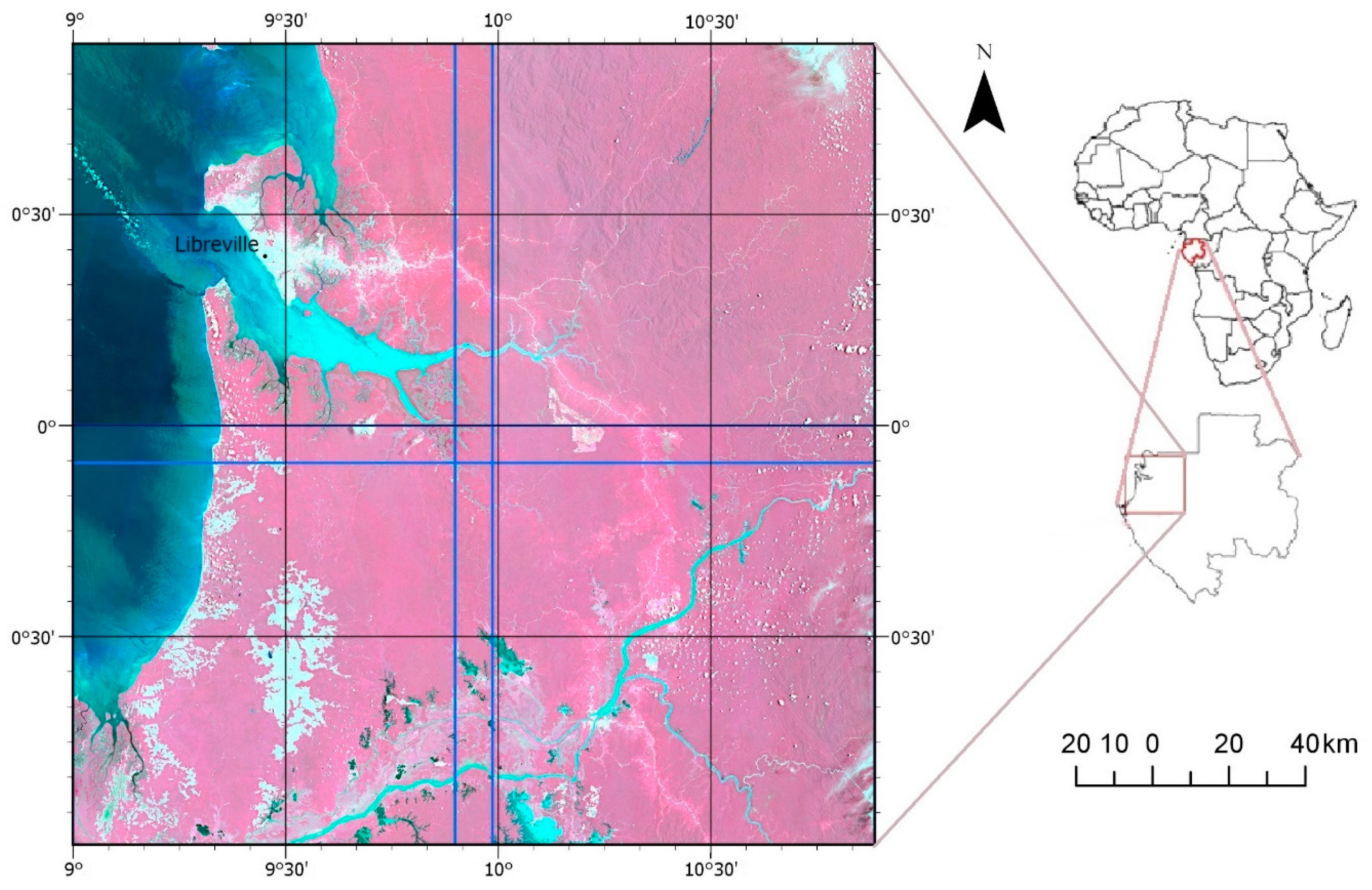
2. Study Area
3. Data
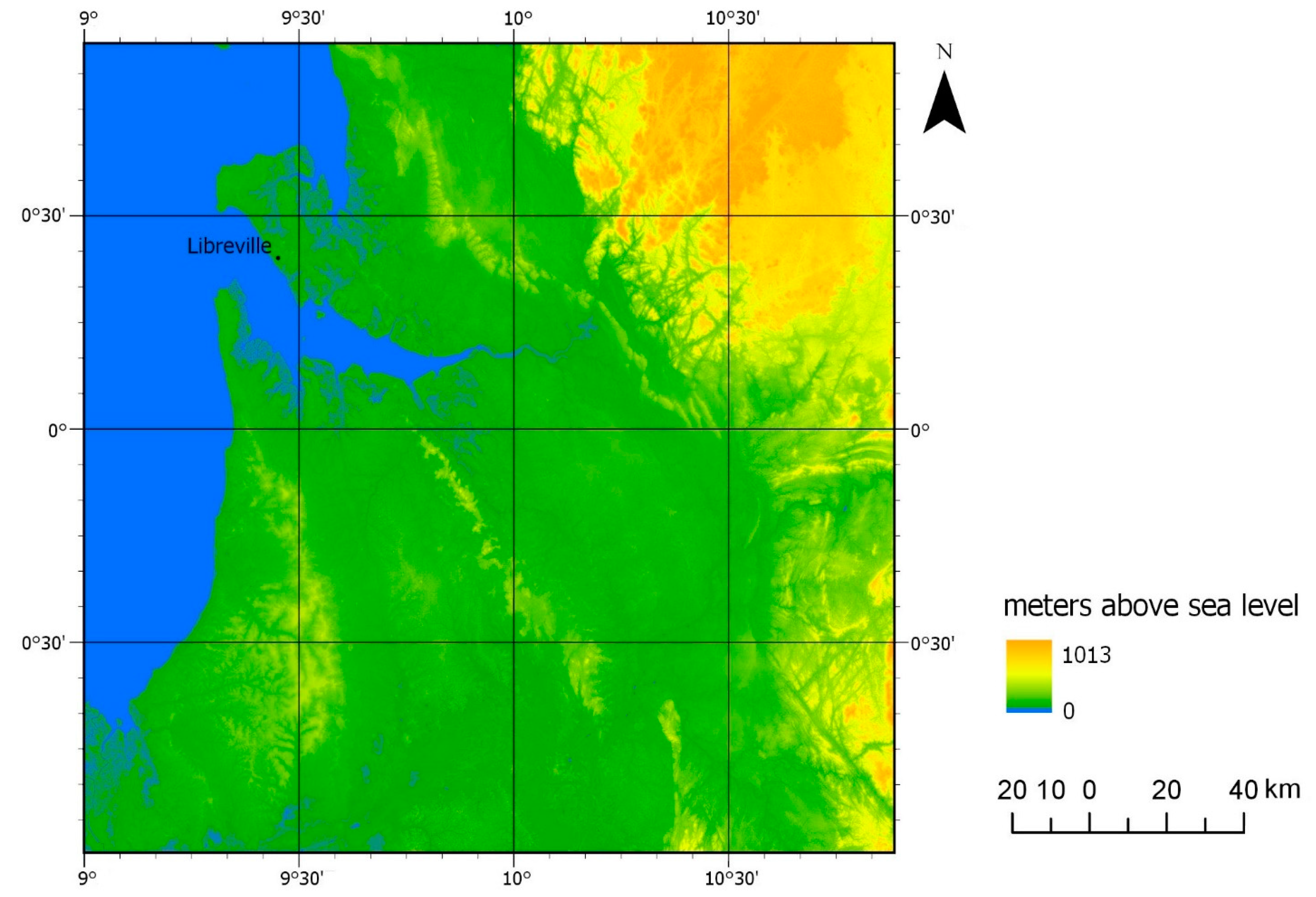
3.1. Sentinel-2 and DEM
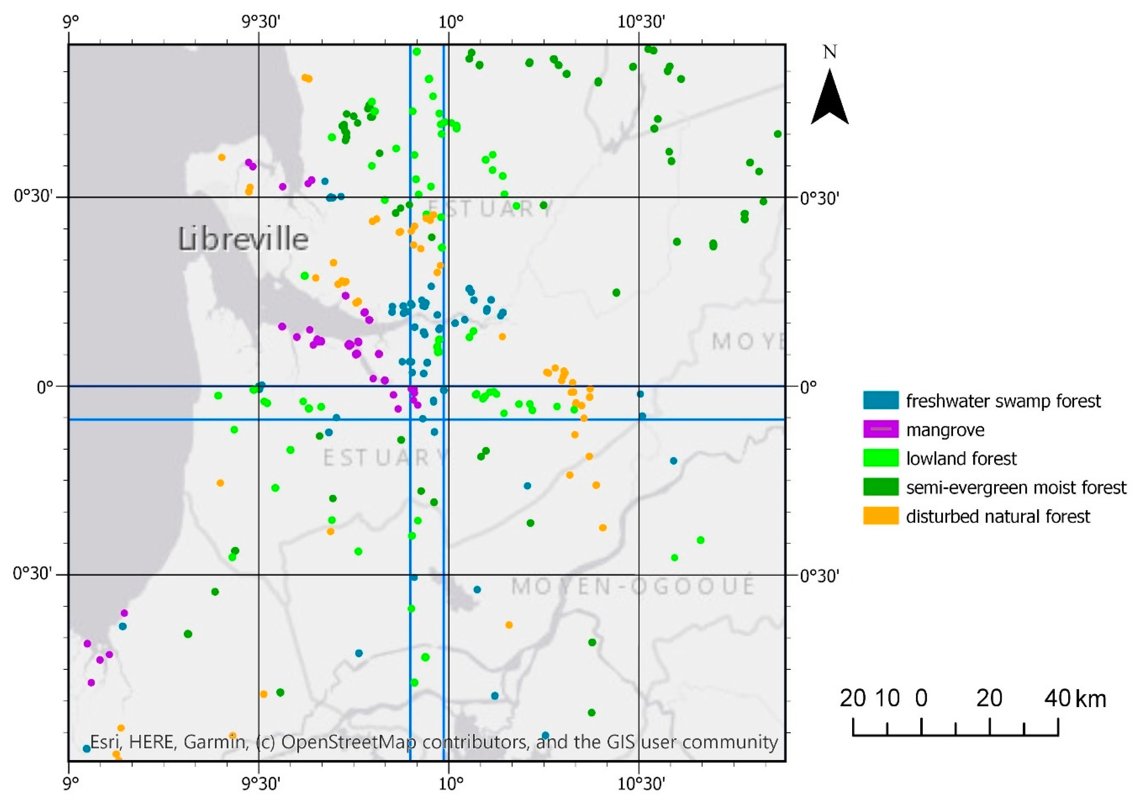
3.2. Reference Datasets
4. Methods
4.1. Selection of Training Samples
4.2. Identification of Forest Types
4.3. Classification Method
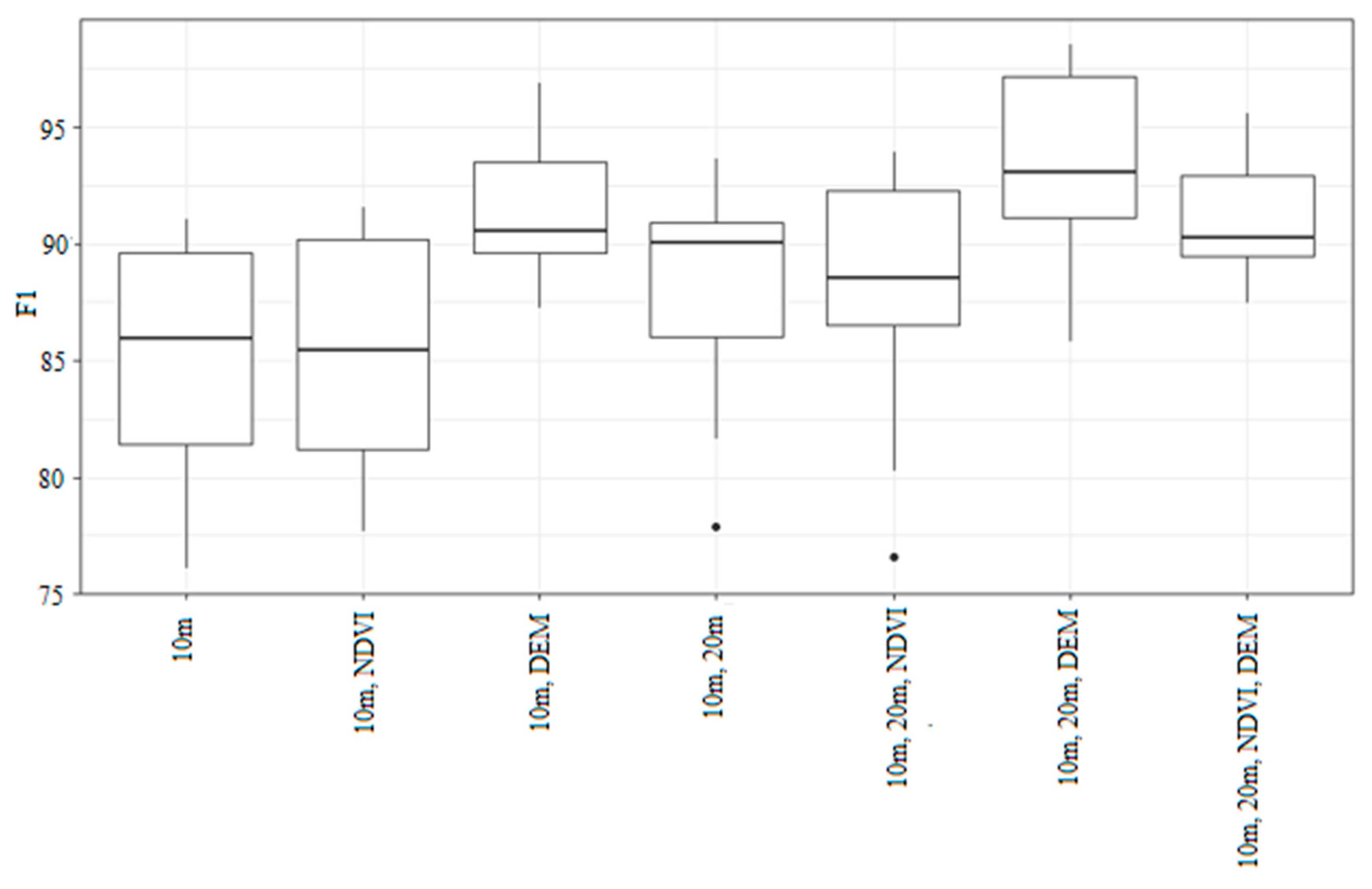
- Bands with a spatial resolution of 10 m (4 variables)
- Bands with a spatial resolution of 10 m and NDVI (5 variables)
- Bands with a spatial resolution of 10 m and DEM (5 variables)
- Bands with a spatial resolution of 10 m and 20 m (10 variables)
- Bands with a spatial resolution of 10 m, 20 m and NDVI (11 variables)
- Bands with a spatial resolution of 10 m, 20 m and DEM (11 variables)
- Bands with a spatial resolution of 10 m, 20 m, NDVI and DEM (12 variables)
4.4. Accuracy Assessment
5. Results
5.1. Forest Cover Classification
5.2. Forest Type Classification
6. Discussion
7. Conclusions
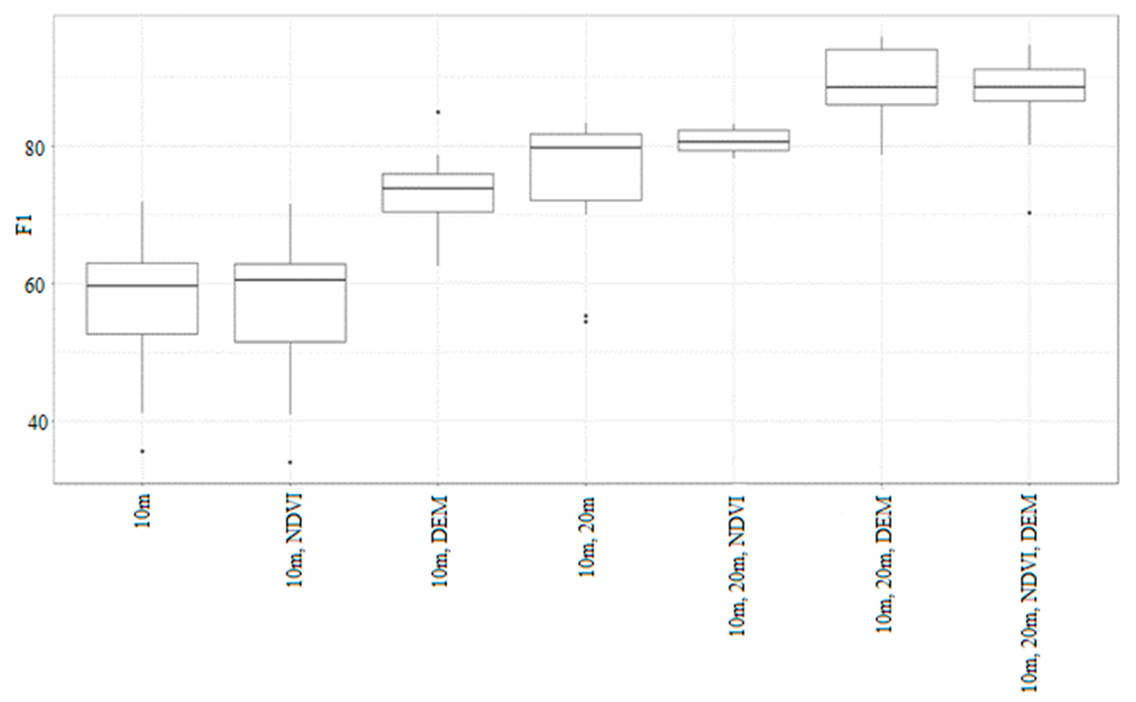
- The highest accuracy for the classification of forest cover and forest type was obtained for the combination of Sentinel-2 bands at 10 m, 20 m spatial resolution and DEM.
- By adding the 20 m bands to the 10 m bands, the accuracy of the classification for both the forest cover and forest type improved significantly.
- The use of the NDVI did not increase the accuracy of the forest cover and type classifications.
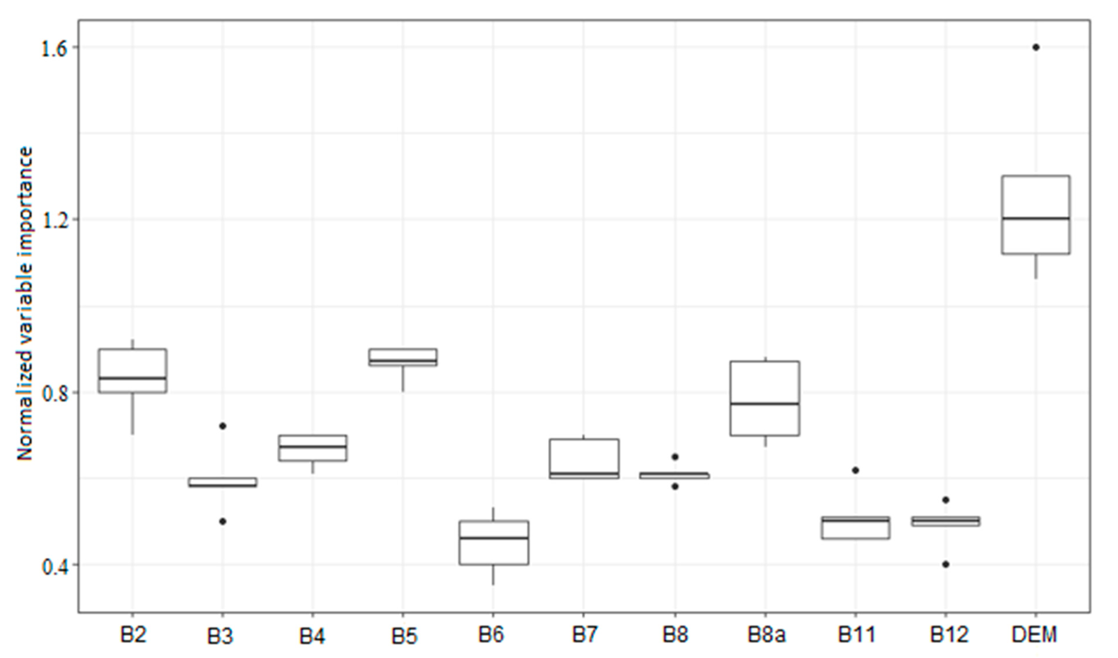
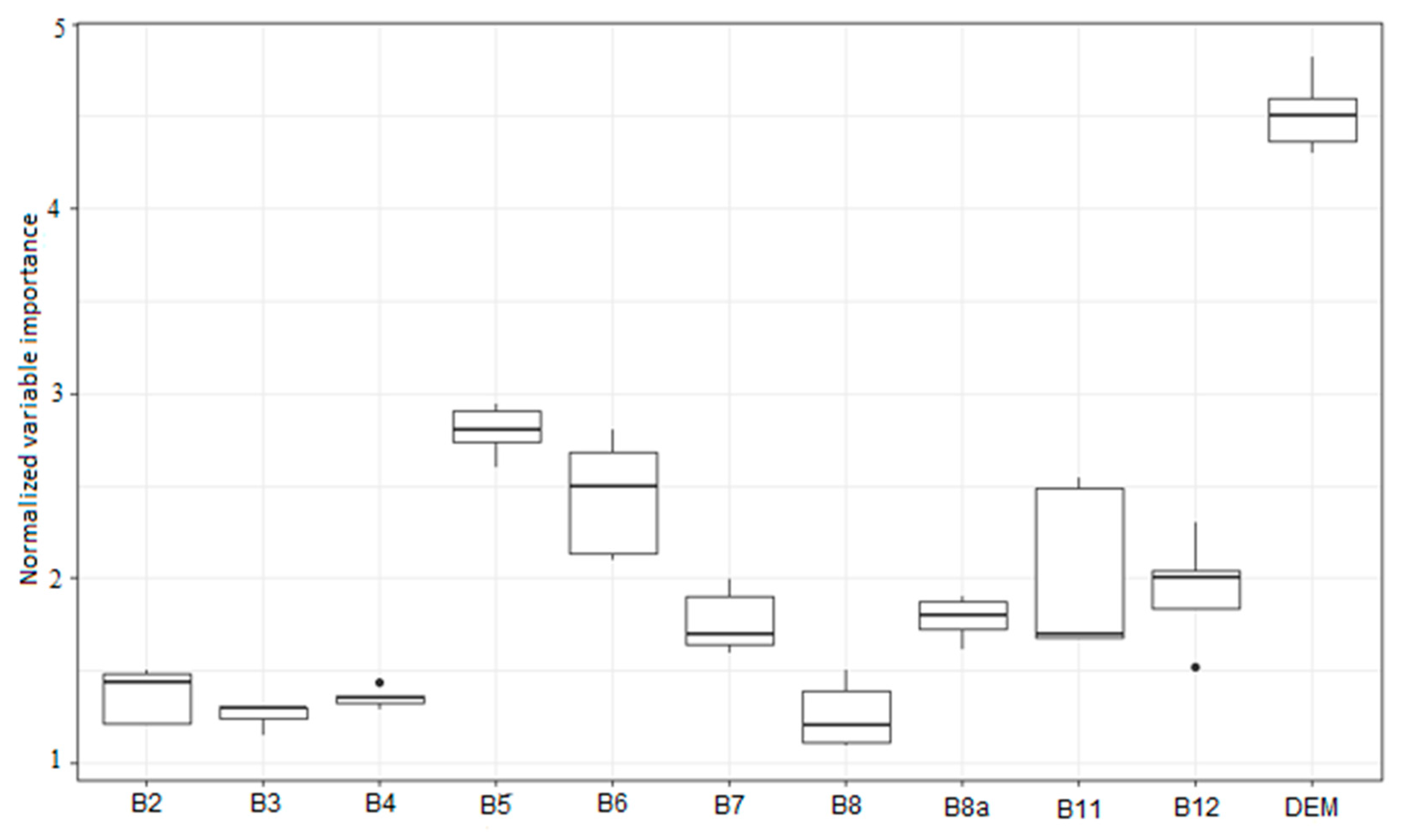
- DEM was demonstrated to be the most important variable in the classification of forest type.
- Among the Sentinel-2 spectral bands, the red-edge B5 and B6, followed by the SWIR B12, contributed the most to the accuracy of the forest type classification. Interestingly, the 10 m spectral bands, B2, B3, B4 and B8, were the least useful in the classification of forest type.
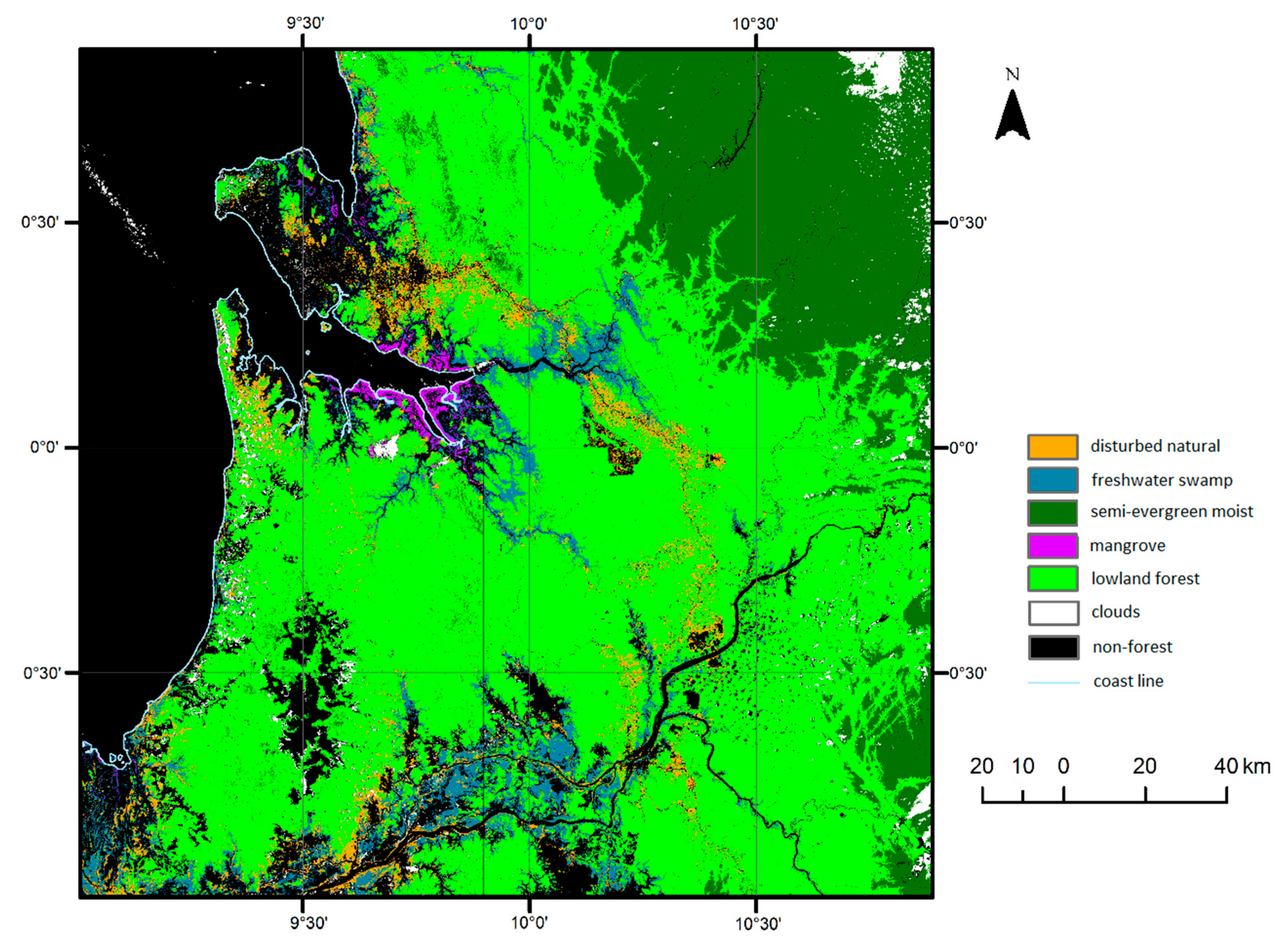
- The mangrove forest was classified with a high accuracy of 98%, followed by lowland forest (96%), disturbed natural forest (85%) and freshwater swamp forest (84%).
- The RF model for forest cover classification was successfully transferred from one master image to other images. In contrast, the transferability of the forest type model was more complex, because of the heterogeneity of the forest types and environmental conditions across the study area.
- The accuracy of the forest type classification was higher for the image used to train the model compared to the image where the model was reused.
- The forest cover and forest type classification models can be successfully reused on other images if the same land cover classes occur in both images.
Author Contributions
Funding
Acknowledgments
Conflicts of Interest
References
- Koppad, A.G.; Janagoudar, B.S. Vegetation analysis and land use land cover classification of forest in Uttara Kannada district India using remte sensing and GIS techniques. ISPRS Int. Arch. Photogramm. Remote Sens. Spat. Inf. Sci. 2017, 42, 121–125. [Google Scholar] [CrossRef]
- Rahman, M.M.; Sumantyo, J.T.S. Mapping tropical forest cover and deforestation using synthetic aperture radar (SAR) images. Appl. Geomat. 2010, 2, 113–121. [Google Scholar] [CrossRef]
- McRoberts, R.E.; Tomppo, E.O. Remote sensing support for national forest inventories. Remote Sens. Environ. 2007, 110, 412–419. [Google Scholar] [CrossRef]
- Wang, Z.B.; Andrew. An integrated method for forest canopy cover mapping using Landsat ETM+ imagery. In Proceedings of the ASPERS/MAPRS2009 Fall Conference, San Antonio, TX, USA, 16–19 November 2009; pp. 16–19. [Google Scholar]
- Hojas-Gascon, L.; Belward, A.; Eva, H.; Ceccherini, G.; Hagolle, O.; Garcia, J.; Cerutti, P. Potential improvement for forest cover and forest degradation mapping with the forthcoming sentinel-2 program. ISPRS Int. Arch. Photogramm. Remote Sens. Spat. Inf. Sci. 2015, 40, 417–423. [Google Scholar] [CrossRef]
- Laurin, G.V.; Puletti, N.; Hawthorne, W.; Liesenberg, V.; Corona, P.; Papale, D.; Chen, Q.; Valentini, R. Discrimination of tropical forest types, dominant species, and mapping of functional guilds by hyperspectral and simulated multispectral Sentinel-2 data. Remote Sens. Environ. 2016, 176, 163–176. [Google Scholar] [CrossRef]
- Fagan, M.E.; DeFries, R.S.; Sesnie, S.E.; Arroyo-Mora, J.P.; Soto, C.; Singh, A.; Townsend, P.A.; Chazdon, R.L. Mapping species composition of forests and tree plantations in northeastern Costa Rica with an integration of hyperspectral and multitemporal landsat imagery. Remote Sens. 2015, 7, 5660–5696. [Google Scholar] [CrossRef]
- Da Ponte, E.; Mack, B.; Wohlfart, C.; Rodas, O.; Fleckenstein, M.; Oppelt, N.; Dech, S.; Kuenzer, C. Assessing forest cover dynamics and forest perception in the Atlantic forest of Paraguay, combining remote sensing and household level data. Forests 2017, 8, 389. [Google Scholar] [CrossRef]
- Noi, P.T.; Kappas, M. Comparison of random forest, k-nearest neighbor, and support vector machine classifiers for land cover classification using sentinel-2 imagery. Sensors 2018, 18, 18. [Google Scholar] [CrossRef]
- Erinjery, J.J.; Singh, M.; Kent, R. Mapping and assessment of vegetation types in the tropical rainforests of the Western Ghats using multispectral Sentinel-2 and SAR Sentinel-1 satellite imagery. Remote Sens Environ. 2018, 216, 345–354. [Google Scholar] [CrossRef]
- Nomura, K.; Mitchard, E.T.A. More than meets the eye: Using sentinel-2 to map small plantations in complex forest landscapes. Remote Sens. 2018, 10, 1693. [Google Scholar] [CrossRef]
- Mercier, A.; Betbeder, J.; Rumiano, F.; Baudry, J.; Gond, V.; Blanc, L.; Bourgoin, C.; Cornu, G.; Ciudad, C.; Marchamalo, M.; et al. Evaluation of sentinel-1 and 2 time series for land cover classification of forest-agriculture mosaics in temperate and tropical landscapes. Remote Sens. 2019, 11, 979. [Google Scholar] [CrossRef]
- Navarro, J.A.; Algeet, N.; Fernandez-Landa, A.; Esteban, J.; Rodriguez-Noriega, P.; Guillen-Climent, M.L. Integration of UAV, sentinel-1, and sentinel-2 data for mangrove plantation aboveground biomass monitoring in Senegal. Remote Sens. 2019, 11, 77. [Google Scholar] [CrossRef]
- Sothe, C.; de Almeida, C.M.; Liesenberg, V.; Liesenberg, V. Evaluating sentinel-2 and landsat-8 data to map sucessional forest stages in a subtropical forest in southern Brazil. Remote Sens. 2017, 9, 838. [Google Scholar] [CrossRef]
- Liu, Y.A.; Gong, W.S.; Hu, X.Y.; Gong, J.Y. Forest type identification with random forest using sentinel-1A, sentinel-2A, multi-temporal landsat-8 and DEM data. Remote Sens. 2018, 10, 946. [Google Scholar] [CrossRef]
- Butler, R.A. Deforestation Statistics for Gabon. Mongabay. 2018. Available online: https://rainforests.mongabay.com/deforestation/archive/Gabon.htm (accessed on 24 June 2020).
- Duveiller, G.; Defourny, P.; Desclee, B.; Mayaux, P. Deforestation in Central Africa: Estimates at regional, national and landscape levels by advanced processing of systematically-distributed Landsat extracts. Remote Sens. Environ. 2008, 112, 1969–1981. [Google Scholar] [CrossRef]
- Montreal, C. Convention on Biological Diversity. Definitions. 2014. Available online: https://www.cbd.int/forest/definitions.shtml (accessed on 24 June 2020).
- Climate—Gabon. Climates to Travel. World Climate Guide. Available online: https://www.climatestotravel.com/climate/gabon (accessed on 24 June 2020).
- Sen2Cor. Science Toolbox Exploitation Platform (STEP). European Space Agency. Available online: http://step.esa.int/main/third-party-plugins-2/sen2cor/ (accessed on 7 July 2017).
- Rouse, J.W.; Haas, R.H.; Scheel, J.A.; Deering, D.W. Monitoring vegetation systems in the great plains with ERTS. In Proceedings of the 3rd Earth Resource Technology Satellite (ERTS) Symposium NASA, Washington, DC, USA, 10–14 December 1973; pp. 309–317, document ID:19740022614. [Google Scholar]
- U.S. Geological Survey. EarthExplorer—Home. Available online: https://earthexplorer.usgs.gov/ (accessed on 7 July 2017).
- Hansen, M.C.; Potapov, P.V.; Moore, R.; Hancher, M.; Turubanova, S.A.; Tyukavina, A.; Thau, D.; Stehman, S.V.; Goetz, S.J.; Loveland, T.R.; et al. High-resolution global maps of 21st-century forest cover change. Science 2013, 342, 850–853. [Google Scholar] [CrossRef]
- Bontemps, S.; Defourny, P.; Van Bogaert, E.; Arino, O.; Kalogirou, V.; Perez, J.R. GLOBCOVER 2009 Products description and validation report. ESA Bull. 2011, 53. [Google Scholar] [CrossRef]
- Breiman, L. Random forests—Random features. Mach. Learn. 2001, 45, 5–32. [Google Scholar] [CrossRef]
- Liaw, A.; Wiener, M. Classification and regression by randomForest. R News 2002, 2, 18–22. [Google Scholar]
- Belgiu, M.; Dragut, L. Random forest in remote sensing: A review of applications and future directions. ISPRS J. Photogramm. Remote Sens. 2016, 114, 24–31. [Google Scholar] [CrossRef]
- Van der Linden, S.; Rabe, A.; Held, M.; Jakimow, B.; Leitão, P.J.; Okujeni, A.; Schwieder, M.; Suess, S.; Hostert, P. The EnMAP-Box-A toolbox and application programming interface for EnMAP data Processing. Remote Sens. 2015, 7, 11249–11266. [Google Scholar] [CrossRef]
- Waske, B.; Van Der Linden, S.; Oldenburg, C.; Jakimow, B.; Rabe, A.; Hostert, P. imageRFeA user-oriented implementation for remote sensing image analysis with Random Forests. Environ. Model. Softw. 2012, 35, 192–193. [Google Scholar] [CrossRef]
- Jakimow, B.; Oldenburg, C.; Rabe, A.; Waske, B.; Van Der Linden, S.; Hostert, P. Manual for Application: Imagerf (1.1); Universität Bonn, Institute of Geodesy and Geo Information, Department of Photogrammetry and Humboldt-Universität zu Berlin, Geomatics Lab.: Berlin, Germany, 2012. [Google Scholar]
- Silveira, E.M.O.; Bueno, I.T.; Acerbi, F.W.; Mello, J.M.; Scolforo, J.R.S.; Wulder, M.A. Using spatial features to reduce the impact of seasonality for detecting tropical forest changes from landsat time series. Remote Sens. 2018, 10, 808. [Google Scholar] [CrossRef]
- Kennaway, T.A.; Helmer, E.H.; Lefsky, M.A.; Brandeis, T.A.; Sherrill, K.R. Mapping land cover and estimating forest structure using satellite imagery and coarse resolution lidar in the Virgin Islands. J. Appl. Remote Sens. 2008, 2, 023551. [Google Scholar] [CrossRef]
- Saini, R.; Ghosh, S. Exploring capablility of Sentinel-2 for vegetation mapping using Random Forest. ISPRS Int. Arch. Photogramm. Remote Sens. Spat. Inf. Sci. 2018, 42, 1499–1502. [Google Scholar] [CrossRef]
- Connette, G.; Oswald, P.; Songer, M.; Leimgruber, P. Mapping distinct forest types improves overall forest identification based on multi-spectral landsat imagery for myanmar’s Tanintharyi region. Remote Sens. 2016, 8, 882. [Google Scholar] [CrossRef]
- Dorren, L.K.A.; Maier, B.; Seijmonsbergen, A.C. Improved landsat-based forest mapping in steep mountainous terrain using object-based classification. For. Ecol. 2003, 183, 31–46. [Google Scholar] [CrossRef]
- Hościło, A.; Lewandowska, A. Mapping forest type and tree species on a regional scale using multi-temporal sentinel-2 data. Remote Sens. 2019, 11. [Google Scholar] [CrossRef]
- Pouteau, R.; Gillespie, T.W.; Birnbaum, P. Predicting tropical tree species richness from normalized difference vegetation index time series: The devil is perhaps not in the detail. Remote Sens. 2018, 10, 698. [Google Scholar] [CrossRef]
- Mutanga, O.; Skidmore, A.K. Red edge shift and biochemical content in grass canopies. ISPRS J. Photogramm. Remote Sens. 2007, 62, 34–42. [Google Scholar] [CrossRef]
- Wessel, M.; Brandmeier, M.; Tiede, D. Evaluation of different machine learning algorithms for scalable classification of tree types and tree species based on sentinel-2 data. Remote Sens. 2018, 10, 1419. [Google Scholar] [CrossRef]
- Immitzer, M.; Atzberger, C.; Koukal, T. Tree species classification with random forest using very high spatial resolution 8-BandWorldView-2 satellite data. Remote Sens. 2012, 4, 2661–2693. [Google Scholar] [CrossRef]
- Van Passel, J.; De Keersmaecker, W.; Somers, B. Monitoring woody cover dynamics in tropical dry forest ecosystems using sentinel-2 satellite imagery. Remote Sens. 2020, 12, 1276. [Google Scholar] [CrossRef]
- Reiche, J.; Verhoeven, R.; Verbesselt, J.; Hamunyela, E.; Wielaard, N.; Herold, M. Characterizing tropical forest cover loss using dense sentinel-1 data and active fire alerts. Remote Sens. 2018, 10, 777. [Google Scholar] [CrossRef]
- Hirschmugl, M.; Deutscher, J.; Sobe, C.; Bouvet, A.; Mermoz, S.; Schardt, M. Use of SAR and optical time series for tropical forest disturbance mapping. Remote Sens. 2020, 12, 727. [Google Scholar] [CrossRef]


| Northwest Image * | Northeast Image | Southwest Image | Southeast Image | |
|---|---|---|---|---|
| Overall accuracy | 94.8 | 92.6 | 98.5 | 98.0 |
| Kappa coefficient | 89.2 | 87.1 | 97.0 | 96.1 |
| UA/PA Forest | 89.7/100 | 77.7/92.1 | 96.2/100 | 80.6/98.1 |
| UA/PA Non-forest | 100/89.7 | 94.5/83.8 | 100/96.1 | 97.5/76.4 |
| Northwest Image * | Southwest Image | Northeast Image * | Southeast Image | |
|---|---|---|---|---|
| Overall accuracy | 95.9 | 90.1 | 97.4 | 83.4 |
| Kappa coefficient | 93.1 | 85.3 | 95.7 | 71.5 |
| UA/PA Disturbed natural forest | 61.5/71.4 | 66.4/80.4 | 100/98.0 | 93.4/84.8 |
| UA/PA Freshwater swamp forest | 60.3/100 | 84.8/91.1 | 89.4/100 | 100/64.9 |
| UA/PA Lowland forest | 96.9/94.5 | 93.6/97.6 | 99.4/93.5 | 76.3/97.9 |
| UA/PA Semi-evergreen moist forest | 99.9/86.9 | 97.5/77.2 | 100/100 | 96.0/67.1 |
| UA/PA Mangroves | 99.9/100 | 96.7/79.9 | NA | NA |
| Disturbed Natural Forest | Freshwater Swamp Forest | Semi-Evergreen Moist Forest | Mangroves | Lowland Forest | |
|---|---|---|---|---|---|
| Disturbed natural forest | 85% | 2% | 0% | 1% | 1% |
| Freshwater swamp forest | 4% | 84% | 0% | 1% | 2% |
| Semi-evergreen moist forest | 2% | 0% | 82% | 0% | 1% |
| Mangroves | 0% | 0% | 0% | 98% | 0% |
| Lowland forest | 9% | 14% | 18% | 0% | 96% |
© 2020 by the authors. Licensee MDPI, Basel, Switzerland. This article is an open access article distributed under the terms and conditions of the Creative Commons Attribution (CC BY) license (http://creativecommons.org/licenses/by/4.0/).
Share and Cite
Waśniewski, A.; Hościło, A.; Zagajewski, B.; Moukétou-Tarazewicz, D. Assessment of Sentinel-2 Satellite Images and Random Forest Classifier for Rainforest Mapping in Gabon. Forests 2020, 11, 941. https://doi.org/10.3390/f11090941
Waśniewski A, Hościło A, Zagajewski B, Moukétou-Tarazewicz D. Assessment of Sentinel-2 Satellite Images and Random Forest Classifier for Rainforest Mapping in Gabon. Forests. 2020; 11(9):941. https://doi.org/10.3390/f11090941
Chicago/Turabian StyleWaśniewski, Adam, Agata Hościło, Bogdan Zagajewski, and Dieudonné Moukétou-Tarazewicz. 2020. "Assessment of Sentinel-2 Satellite Images and Random Forest Classifier for Rainforest Mapping in Gabon" Forests 11, no. 9: 941. https://doi.org/10.3390/f11090941
APA StyleWaśniewski, A., Hościło, A., Zagajewski, B., & Moukétou-Tarazewicz, D. (2020). Assessment of Sentinel-2 Satellite Images and Random Forest Classifier for Rainforest Mapping in Gabon. Forests, 11(9), 941. https://doi.org/10.3390/f11090941