Estimation of Future Changes in Aboveground Forest Carbon Stock in Romania. A Prediction Based on Forest-Cover Pattern Scenario

Abstract

The aboveground forest biomass plays a key role in the global carbon cycle and is considered a large and constant carbon reservoir. Hence, exploring the future potential changes in forest-cover pattern can help to estimate the trend of forest biomass and therefore, carbon stock in a certain area. As a result, the present paper attempts to model the potential changes in aboveground forest carbon stock based on the forest-cover pattern scenario simulated for 2050. Specifically, the resulting aboveground forest biomass, estimated for 2015 using the allometric equation based on diameter at breast height and the estimated forest density, was used as baseline data in the present approach. These spatial data were integrated into the forest-cover pattern scenario, predicted by using a spatially explicit model, i.e., the Conversion of Land Use and its Effects at Small regional extent (CLUE-S), in order to estimate the potential variation of aboveground forest carbon stock. Our results suggest an overall increase by approximately 4% in the aboveground forest carbon stock until 2050 in Romania. However, important differences in the forest-cover pattern change were predicted on the regional scale, thus highlighting that the rates of carbon accumulation will change significantly in large areas. This study may increase the knowledge of aboveground forest biomass and the future trend of carbon stock in the European countries. Furthermore, due to their predictive character, the results may provide a background for further studies, in order to investigate the potential ecological, socio-economic and forest management responses to the changes in the aboveground forest carbon stock. However, in view of the uncertainties associated with the data accuracy and methodology used, it is presumed that the results include several spatial errors related to the estimation of aboveground forest biomass and simulation of future forest-cover pattern change and therefore, represent an uncertainty for the practical management of applications and decisions.

1. Introduction

The largest perturbation to Earth’s radiation budget is caused by the increases in the abundances of the long-lived and well-mixed greenhouse gases [1]. Among these greenhouse gases, carbon dioxide (CO₂) from fossil fuel burning and human induced land-use change is the most important single anthropogenic influence; its effect on climate change becoming a key global environmental issue [2]. This could have significant negative impacts on terrestrial ecosystems with many implications for sustainability, biodiversity and the provision of ecosystem goods and services to people [3]. Ecosystems are a net carbon sink, removing CO₂ from the atmosphere, when plant photosynthesis exceeds the sum of respiration and combustion, and a source when the sum of respiration and combustion exceeds photosynthesis [3]. Forest ecosystems are increasingly recognized as important elements of the global carbon cycle [4], their dynamics being a great global concern due to the role they play in climate change [5]. Forests become sources of atmospheric CO₂ when impacted by human or natural disturbances, but they can also function as carbon sinks in order to sequester or preserve significant quantities during regrowth after disturbance [6]. As a result of their importance in the carbon cycles, the United Nations Framework Convention on Climate Change, and in particular the Kyoto Protocol recognize the importance of forest carbon sinks and the need to monitor, preserve and enhance terrestrial carbon stocks through afforestation and reforestation [7]. Forests account for 70–90% of the terrestrial aboveground and belowground biomass, while the aboveground forest biomass makes up 70–90% of the total forest biomass [8]. Therefore, the aboveground forest biomass is an important indicator for forest carbon storage and sequestration of forests [9], as well as for estimating potential emissions from land cover changes (forest fragmentation, deforestation, reforestation, afforestation), and biotic and abiotic disturbances [10]. However, due to the spatial and temporal variation of the aboveground forest biomass, the global distribution of carbon sinks remains uncertain [11].

In recent decades, the estimation of aboveground forest biomass has become an important way to estimate aboveground forest carbon stock. The carbon content of trees is usually calculated from wood volume equations that include basic wood density and a conversion factor for the carbon concentration (%) in dry biomass [12]. In general, the carbon content of trees varies widely among species and wood quality, but a concentration ratio of 50% is proposed to be used as a default value by the IPCC [12]. Furthermore, a carbon concentration ratio of 50% is used to convert dry tree biomass to carbon stock at an operational level [13].

Aboveground forest biomass is defined as “the aboveground standing dry mass of live or dead matter from tree or shrub life forms, expressed as a mass-per-unit area” [14], typically Mg ha^–1. Aboveground forest biomass can only be directly measured with destructive harvesting [15], but this direct estimation is rarely practical because it is complex, expensive and time-consuming. In practice, even though field-based techniques take up more resources and time, they are more effective compared to other methods [16]. However, because they provide data for a limited number of trees and species, these methods might not be representative for estimating the aboveground forest biomass over large areas. For these reasons, aboveground forest biomass is often inferred through the use of allometric equations that associate more easily-measured parameters [15], such as diameter-at-breast-height (dbh), usually measured at 1.3 m above the ground, tree height (th) or a combination of the two [17]. Hence, biomass models which relate different tree biomass components to dendrometrical variables and biomass expansion factors are particularly useful tools in aboveground forest biomass estimation [18,19]. In the past decades, aboveground forest biomass estimation is usually carried out using ‘indirect’ methods, based on the remote sensing techniques, because satellite imagery provides consistent global vegetation coverage at a relatively high spatial resolution [20,21]. In particular, the estimation of aboveground forest biomass using Light Detection and Ranging (LiDAR) scanning is highlighted in many studies (e.g., [22,23,24,25]) because it provides an unprecedented opportunity to capture high resolution [15] and furthermore, the estimation of the volume for individual trees with increased accuracy. In addition, the combination between remote sensing and LiDAR technology can provide more advantages for mapping the aboveground forest biomass [25].

Estimates of aboveground forest biomass using remote sensing methods are typically generated through a combination with field sampling [26]. Specifically, this technique initially requires an extensive destructive sampling to establish allometric models, and the models can be used as a non-destructive method to estimate tree biomass [27]. Thus, finding an already existing equation for the geographically closest site is required in order to estimate aboveground forest biomass on a large spatial scale [28]. Several authors have reported that generalized regressions developed from field measurements can reasonably estimate the aboveground forest biomass from other sites (e.g., [29,30]). However, the accuracies of remote sensing-based aboveground forest biomass maps are inherently dependent on the underlying accuracies of the field estimates of biomass that are used to calibrate remote sensing-based models [31]. Furthermore, the accuracies of these allometric models outside their areas of development remain largely unknown due to a dearth of available sampled validation data [32]. Nevertheless, remote sensing methods are preferred because it is less time consuming and less expensive [33], and can exhibit spatially explicit patterns of forest biomass and its temporal change [34]. Accordingly, remote sensing methods, based on allometric equations, have been widely applied to estimate the aboveground forest biomass across a range of scales, from local to continental (e.g., [35,36,37,38,39,40]).

The aboveground forest biomass of European countries has been systematically inventoried, including different estimation methods (e.g., [7,30,41,42]) at regional and national scale. To date, spatial estimates of the aboveground forest biomass and its distribution at national scale are not well known in Romania. However, a national report of the aboveground forest biomass quantity is regularly prepared in order to monitor forests and their management through the FAO (Food and Agriculture Organization)’s Global Forest Resource Assessment [43], but the estimation is based on the statistical information of the total above ground volume and wood density of coniferous and broadleaved forests. The aboveground forest biomass models created by the use of allometric relations have been established (e.g., [44,45]), although only on a local scale and for young broadleaved trees plantations. In addition, the height and diameter of growth were also estimated for Abies alba Mill., Fagus sylvatica L. and Picea abies L. Karst [46], in order to measure the average annual stem volume growth in different local environments. At national scale, an aboveground forest biomass model based on remote sensing data was developed in the Holistics of the Impact of Renewable Energy Sources on Environment and Climate (HORESEC) Project and published by [47]. The map was the result of allometric equations using the dbh as an independent variable, but due to the unavailability of plot-level measurements, the resulting values were not yet validated by comparing the model with independent test data.

Further changes in human-induced land-use disturbances could influence the spatial and temporal variability of aboveground forest biomass and the rate of carbon accumulation and could therefore, present a major risk to climate change mitigation efforts [48]. However, future land-use/cover pattern change predictions may help us understand the carbon sink trend, especially by modeling potential areas with forest gain and loss. Different models have been developed in order to project land-use/cover dynamics, motivated by several potential benefits [49]: understanding how determining factors trigger land-use/cover changes, generating future scenarios, predicting the location of changes and supporting the design of policy responses to these changes. One of the most used models is the Conversion of Land Use and its Effects at Small regional extent (CLUE-S) [50], which aims to understand and predict the impact of biophysical and socio-economic factors on land-use systems [51].

In the present day, the forest-cover area in Romania constitutes almost 1% of the total forested area in Europe and 4.5% of the total forested area of EU countries [52]. However, over the last decades, forest-cover has been one of the most affected by human-induced land-use change, with the key factors being mostly related to institutional, political and economic drivers. Thus, many studies have reported significant regional forest-cover changes, mainly indicating increased deforestation rates (e.g., [53,54,55,56,57]). Furthermore, a recent forest-cover pattern change scenario in Romania [58] suggests an overall increasing trend in forest-cover area in the near future, mainly in mountain areas, as a result of the decrease in human pressure and/or in relation to environmental changes. At the same time, important forest loss is predicted for the tableland, plateau and for plain regions, mainly as a result of them being converted into agricultural lands or artificially expanded areas. These changes may point to possible environmental implications, having consequences in habitat fragmentation and leading to the occurrence of natural hazardous phenomena [55,58], and forest management [59]. Furthermore, important regional changes in the quantity of aboveground forest biomass and therefore, of carbon sequestration, may also come to be in the area. In this regard, the main objective of the paper is to transpose an estimated aboveground forest biomass quantity into the simulated potential forest-cover pattern change, in order to calculate future potential aboveground forest biomass gain and loss. Based on the resulting changes, we attempt to estimate future aboveground forest carbon stock at national scale and to assess their regional variation. To achieve this, two spatial baseline data have been integrated into a GIS (Geographic Information System) spatial and statistical analysis, i.e., the aboveground forest biomass estimated for 2015 using remote sensing data and the biomass allometric model, and the forest-cover pattern scenario projected for 2050 through the CLUE-S (Conversion of Land Use and its Effects at Small regional extent) model.

2. Materials and Methods

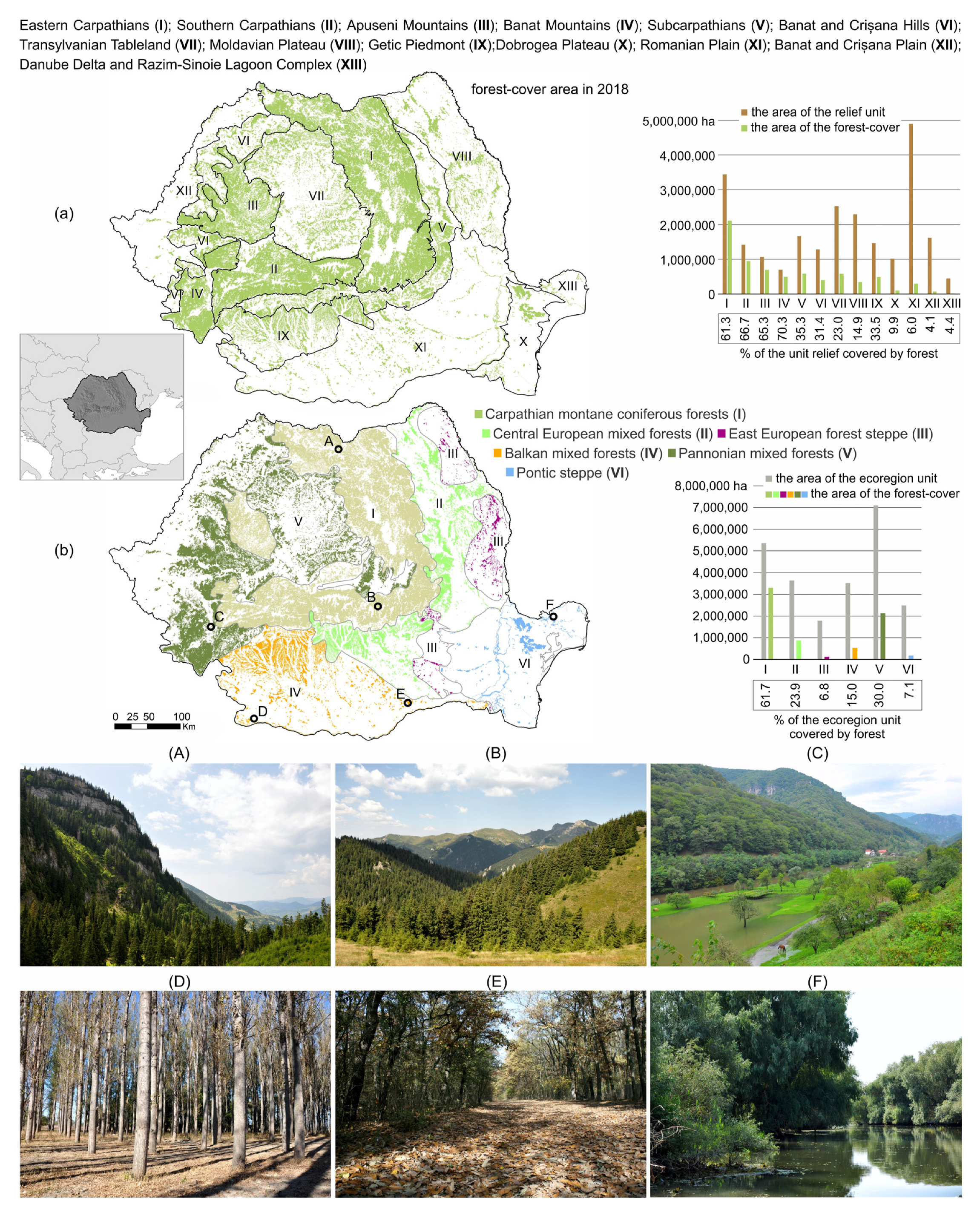
2.1. Study Area

Romania is a medium-sized European state (about 23.84 mil. ha) located in the South-Eastern part of Central Europe, characterized by various landform units, including the largest part of the Carpathian Mountains (57%), surrounded by extended hilly units, and large tableland, plateau and plain areas (Figure 1). With a total area of about 7.13 mil. ha [60], forests make up the dominant land-use/cover category, covering about 29.9% of the total study area. However, the variety of relief forms, coupled with climatic features, the diversity of soil types, socio-economic conditions and land-use history generate significant disparities pertaining to regional forests. Hence, the largest areas (Figure 1a) are extended in the Eastern Carpathians (2.11 mil. ha, that is 29.6% of the total), Southern Carpathians (0.95 mil. ha, that is 13.3% of the total), Apuseni Mountains (0.70 mil. ha, that is 9.8% of the total), Subcarpathians (0.59 mil. ha, that is 8.2% of the total) and Banat Mountains (0.49 mil. ha, that is 6.9% of the total). The smallest areas are located in the Danube Delta and Razim-Sinoie Lagoon Complex (0.02 mil. ha, that is 0.3% of the total), Banat and Crișana Plain (0.07 mil. ha, that is 0.9% of the total), Dobrogea Plateau (0.10 mil. ha, that is 1.4% of the total), Romanian Plain (0.30 mil. ha, that is 4.1% of the total), Moldavian Plateau (0.34 mil. ha, that is 4.8% of the total), Banat and Crișana Hills (0.40 mil. ha, that is 5.6% of the total), Getic Piedmont (0.49 mil. ha, that is 6.9% of the total) and the Transylvanian Tableland (0.58 mil. ha, that is 8.2% of the total). Relative to the overall major relief unit surface, the highest percentage of forest-cover was calculated for the Banat Mountains (70.3%), the Southern Carpathians (66.7%), Apuseni Mountains (65.3%), the Eastern Carpathians (61.3%) and the Subcarpathians (35.3%), while the lowest was registered for the Banat and Crișana Plain (4.1%), the Danube Delta (4.4%) and the Romanian Plain (6%).

The Romanian forests are ecologically highly diverse, these being included in six major vegetation ecoregions [61] (Figure 1b): Carpathian montane coniferous forests (3.31 mil. ha, 46.4% of the total), Pannonian mixed forests (2.13 mil. ha, 29.8% of the total), Central European mixed forests (0.87 mil. ha., 12.2% of the total), Balkan mixed forests (0.53 mil. ha., 7.4% of the total), Pontic steppe (0.18 mil. ha, 2.5% of the total) and East European forest steppe (0.12 mil. ha, 1.7% of the total). Relative to the overall major vegetation ecoregions surface, the highest percentage of forest-cover area was calculated for the Carpathian montane coniferous forests (61.7%), Pannonian mixed forests (30.0%) and Central European mixed forests (23.9%), while the lowest was registered for the East European forest steppe (6.8%) and the Pontic steppe (7.1%).

Overall, deciduous species constitute a dominant forest vegetation (about 70%), including beech (48%), different oak species (23%), other hardwoods (21%) and softwoods (7.4%) [62], widely distributed up to 1000–1200 m a.s.l. The coniferous forests, distributed predominantly in the mountain regions, account for about 30% of the total afforested area, of which spruce trees represent 77%, fir—15% and other coniferous species—7% [62].

The Romanian forests represent an important part of Europe’s natural resources including some of the largest continuous temperate forests [63], that preserve one of the largest stretches of old-growth forest (about 210,000 ha) in Europe [64]. Hence, forest conservation is one of the high priorities in the national forestry legislation, large areas being included in various protected areas (National and Natural Parks, Biosphere Reserves, Scientific and Nature Reserves, RAMSAR Convention on Wetlands of International Importance and Network of Nature Protection Areas Sites —NATURA 2000), in order to preserve biodiversity and to reduce man’s impact [65]. However, forest-cover change is considered among the major environmental concerns in Romania, the region experiencing a continuous decreasing in forest-cover area mainly since 1990 when the breakdown of socialism led to significant changes in land-use/cover structure and pattern. The evolution of forest-cover areas was mostly influenced by legislative factors that led to the restitution of over 45% of the total forest surface (through the laws adopted in 1991, 2000 and 2005) [66,67]. Furthermore, the economic hardships and weakened institutions of the transition period [68,69], as well as the shadow businesses coupled with corruption [70] led to massive forest exploitation, including both legal and illegal logging [53,57]. Therefore, increased deforestation rates have been reported after 1990, and particularly after 2000 at national and regional scale, (e.g., [56,57,58,71,72,73,74]), resulting not only in regionally important forest area decreases, but also in the significant loss of valuable ecosystems and old-growth forests [75]. In contrast, the expansion of the forest-cover area was also recorded in relation to the natural or artificial regeneration. The artificial afforestation and re-afforestation were mainly directly dependent on the financial sources provided by the different projects and programmes, [57,58,76], mostly accessed in the pre- and post-accession to the European Union. Furthermore, changes in land-use and land management have also been indicated as the main influences of forest re-growth. Thus, with the decline of traditional activities, land abandonment and a rise in conservation initiatives [57,77], forests are allowed to re-grow into their potential habitat, mainly in large mountain areas.

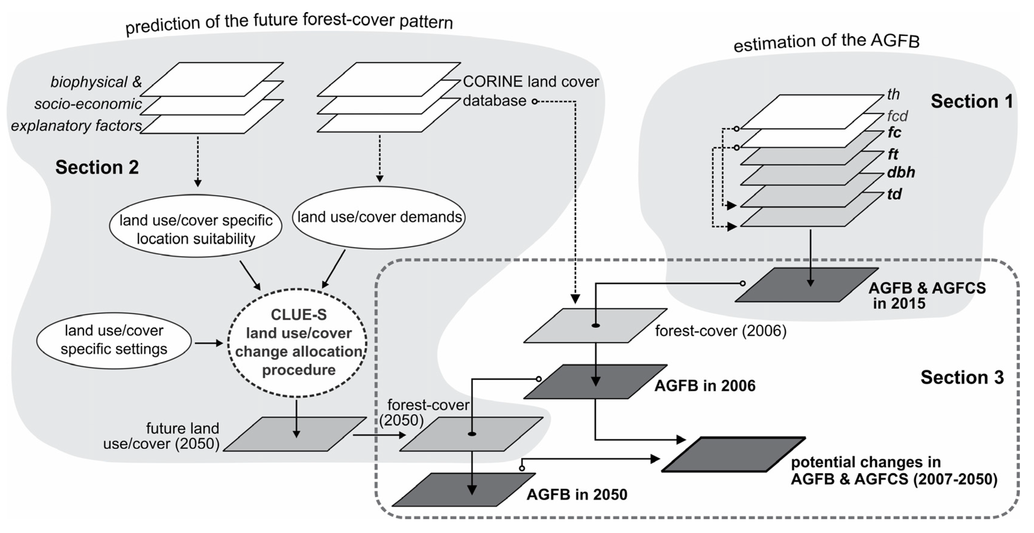
2.2. The Methodology Used to Predict Future Potential Changes in Aboveground Forest Carbon Stock

In order to predict future potential changes in aboveground forest carbon stock (AGFCS), the current analysis uses two baseline datasets. The first one is a raster-data of the aboveground forest biomass (AGFB) for 2015, conducted according to the framework of Holistics of the Impact of Renewable Energy Sources on Environment and Climate (HORESEC, cmu-edu.eu/horesec/). The second information is a raster-data of the forest-cover pattern change scenario for 2050, issued according to the framework of RO-RISK (National Risk Assessment, gis.ro-risk.ro/site/).

Next, a synthetically conceptual model is presented (Figure 2, Sections 1 and 2) and a short overview of the methodological approach used to estimate AGFB and to predict the forest-cover pattern change scenario, but a more detailed description can be found in [47] and [58], respectively. Using these two baseline raster-data, we attempted to model the future potential variations in AGFCS quantity until 2050 by proposing a simple methodological approach presented in Figure 2, Section 3.

In order to quantify and discuss the resulting values according to the regional forest-cover distribution, the analysis was done in accordance with the major relief units in Romania [78] and with the major vegetation ecoregions classified in the map of European Ecological Regions [61]. Thus, the situation in 13 major relief units and 6 major vegetation ecoregions (Figure 1) has been investigated in the present study.

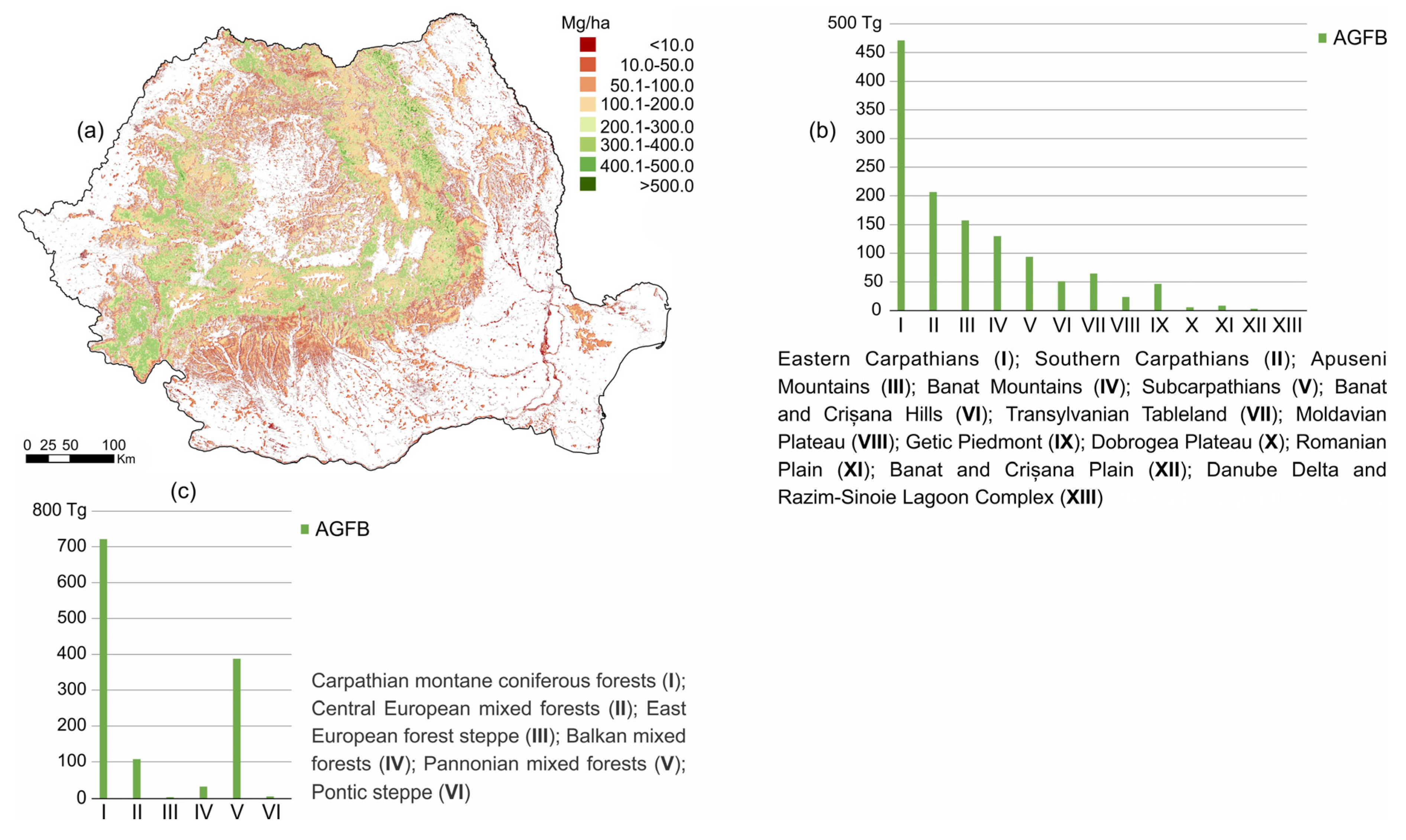
2.2.1. The Estimation of AGFB in 2015

To estimate the AGFB quantity, the spatial information on forest vegetation cover and dominant forest categories, and corresponding area of tree height and forest canopy density (Figure 3) was used in the analysis [47]. The data of forest vegetation cover and dominant forest types, derived from the database available at Copernicus Land Monitoring Service, with a resolution of 20 m, were used to obtain the forest-cover distribution (fc) and the dominant forest types (ft) (i.e., deciduous and coniferous) in the area. The forest height information for 2008, derived from the Carbon Monitoring System Project database (available at the National Aeronautics and Space Administration), with a resolution of 1 km, was used to estimate tree height (th), the indicator used to estimate the diameter at breast height (dbh). Additionally, the data of forest canopy density (fcd) in 2015 derived from the database available at Copernicus Land Monitoring Service, with a resolution of 20 m, was also considered as a variable used to estimate tree density.

Biomass Equations

The AGFB was calculated using the allometric equations and coefficients presented in [42]. This represents the result of the European study Multi-source inventory methods for quantifying carbon stocks and stock changes in European forests’—CarboInvent, where a series of generalized allometric equations have been developed for the most common tree species (Picea abies, Pinus sylvestris, Betula spp., Quercus spp., Fagus spp.).

Based on dbh as a unique predictor, and scaling coefficients for the considered tree species, the allometric equation (Equation (1)) developed by [79,80] was applied to estimate the presented AGFB model:

$$y_i=exp({\beta }_0+{\beta }_1\cdot \frac{dbh}{dbh+{\beta }_2})$$

(1)

where y is the aboveground biomass of the tree i (in kg); dbh is the diameter at breast height (in cm); β₀, β₁ and β₂ are the scaling coefficients that depend on the type of analyzed tree.

In this approach, the dbh was used as the only predictive variable because it is the most common and the easiest to measure in the field [42,81]. This was determined by using the Equation (2) that describes the dbh-th relationship developed by [82] and fitted by [42] for the most common tree species in the European temperate zone:

$$th=1.3+\frac{db{h}^2}{{(X_0+X_1\cdot dbh)}^2}$$

(2)

where th is the tree height (in m); dbh is the diameter at breast height (in cm); X₀ and X₁ are the scaling coefficients for the tree species applied to determine dbh according to the th.

Next, knowing the tree height value in the th raster-data, dbh has been derived from equation no. 2 by applying the Equation (3):

$$dbh=\frac{X_0\sqrt{th-1.3}}{1-X_1\sqrt{th-1.3}}$$

(3)

where dbh is the diameter at breast height (in cm); X₀ and X₁ are the scaling coefficients for the tree species applied to determine dbh according to the th; th is the tree height (in m).

The values of scaling coefficients were extracted from the study of [42] where the generalized allometric equation models for certain tree species in Europe are presented. As a result that we used forest type datasets that contain only the two major classes (deciduous and coniferous forests), we chose to use the scaling coefficients determined for Fagus spp. and Picea abies as representative to compute the AGFB models for the deciduous and coniferous tree species. The reason for the choice was that these two forest species represent the largest distribution in the area: about 48% within deciduous forests (37% of the total forest-cover area) and 77% within coniferous forests (17% of the total forest-cover area) respectively [62]. Although the resulting values are associated with a series of uncertainties, the method used is considered applicable on a national scale in European countries in temperate and boreal areas [22].

The AGFB quantity in a cell of 100 × 100 m was calculated as the product of AGFB quantity/tree (in kg) and the estimated tree density (td) values, and expressed in Mg/ha⁻¹.

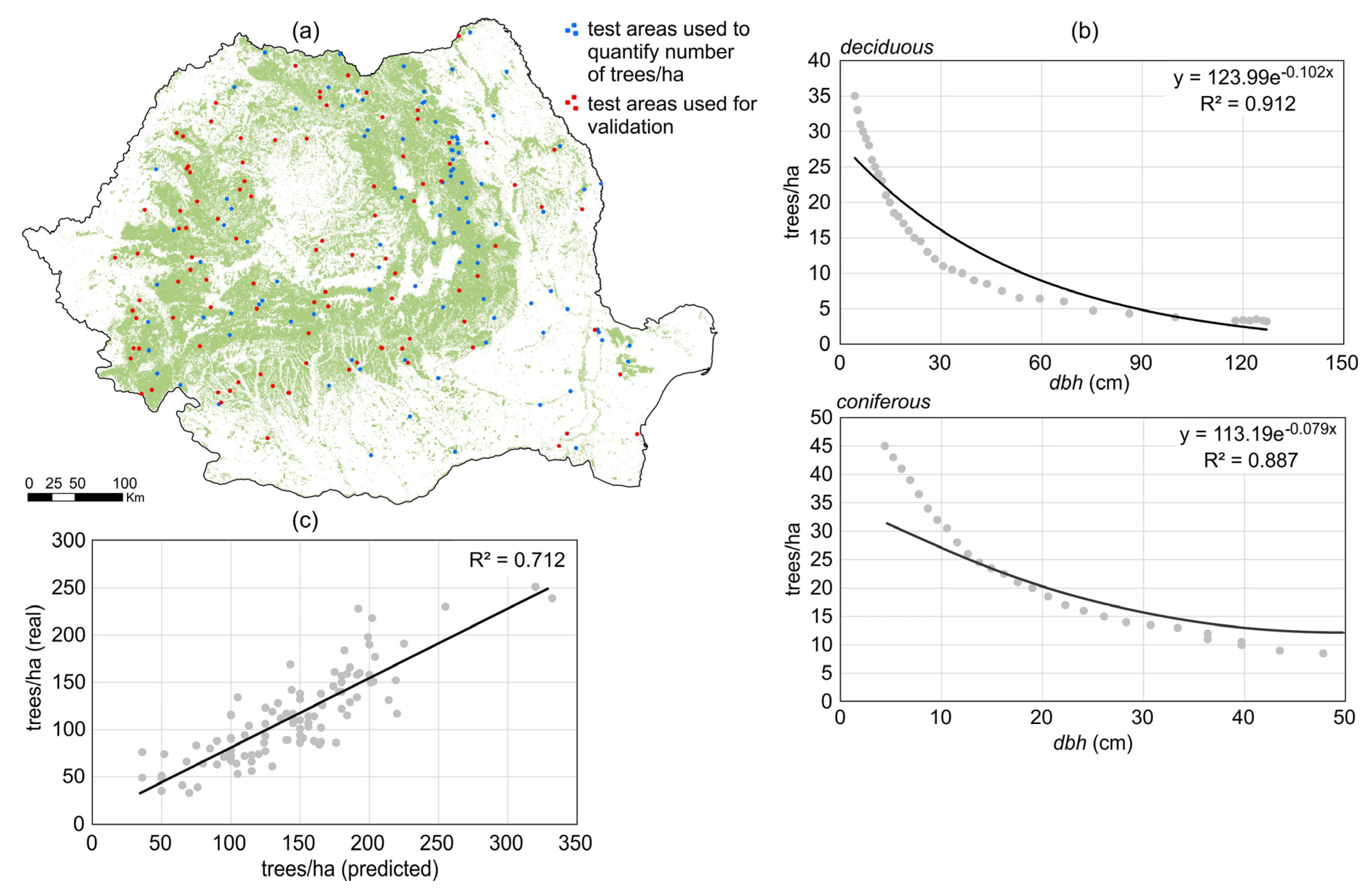
The Estimation of td

To estimate td, two procedures were used in the analysis. The first one defines the relationship between the number of trees and dbh in a certain area. This was statistically determined by quantifying the total number of trees on the ground and the corresponding estimated dbh. To this, the number of trees was visually quantified on the high-resolution satellite images/aerial photography (2018) provided by Google Earth, by using test areas randomly distributed across the forest-cover raster. Specifically, 200 test areas, with a 1 ha window size, were generated (Figure 4a): 100 for the quantification of the number of trees, and 100 to calculate the goodness of fit of the resulting data. Accordingly, a strong inverse exponential relationship between the dbh and the number of trees was found for both deciduous and coniferous species. Therefore, the described functions (Figure 4b) were taken into account to predict the number of trees with unknown values within a cell, by using the observed dbh value.

In the second procedure, the predicted number of trees/ha, obtained for each forest type category, was weighted with the fcd data (Equation (4)) in order to estimate the td:

$$t{d}_i=n{t}_i\cdot \frac{fcd}{100}$$

(4)

where td is the estimated tree density (per ha) for forest type category i; nt is the number of trees predicted for forest type category i according to the dbh values; fcd is the forest canopy density.

Accordingly, the agreement between the real numbers of trees quantified on the ground and predicted td in the 100 test areas used for validation was expressed by the correlation coefficients (Figure 4c). Thus, the obtained R²-value of 0.71 suggests that the obtained data are reasonably accurate and therefore, the estimated td was used to determine the AGFB quantity per ha.

In the end, to indicate the total AGFB, the estimated values per ha (in Mg) were cumulated and converted to Tg for further analysis in accordance with the regional distribution of forest-cover area.

2.2.2. The Estimation of Aboveground Forest Carbon Stock

To estimate the AGFCS amount, the obtained AGFB values were multiplied with the coefficient of 0.5 (Equation (5)), assuming a value of 50% carbon concentration in the total aboveground forest biomass quantity [12,13].

$$AGFCS=AGFB\cdot 0.5$$

(5)

where AGFCS is the aboveground forest carbon stock; AGFB is the aboveground forest biomass.

2.2.3. Modeling Forest-Cover Pattern Change

A future scenario of forest-cover pattern, resulted by simulating land-use/cover change in 2006–2050 [58], was used to estimate future potential changes in AGFCS quantity. The data were predicted using CLUE-S, an empirical multiscale model based on advanced statistical land-use change [50], developed for the spatially explicit simulation [83]. Two datasets were included in the simulation [58]. Firstly, to formulate a baseline scenario, as well as to prepare the further simulated land-use/cover categories and the initial time step (“year 0”) and to validate the results, the CORINE Land Cover (CLC) datasets (accessible via the Copernicus Programme–Copernicus Land Monitoring Service) were used for 1990, 2000, 2006 and 2012. Secondly, to explain the spatial pattern of land-use/cover change, 18 determinant factors of change were included in the modeling [58]. Specifically, the elevation and slope declivity (derived through the Digital Elevation Model—30 m resolution), the average annual precipitation and the average annual temperature in the 1961–2015 period (derived from the spatial data provided by the National Meteorological Administration), horizontal relief fragmentation (derived through EU-Hydro River Network data) and the total organic matter content in topsoil (derived from the map provided by “Romania—Soil quality and electricity transmission grid. Geographical atlas”) were selected for the biophysical factors. For the socio-economic, 12 factors were considered: the population density, the number of employees, the unemployment rate, the employment rate in the tertiary sector, large livestock units and the built-up/non-agricultural ratio in 2006, as well as the population growth between 1992–2006 (derived from the statistical data provided by the National Institute of Statistics), settlements density and distance to settlements in 2006 (derived by CORINE Land Cover dataset), distance to nearest main towns (derived from the statistical data provided by the National Institute of Statistics) and the density of the secondary roads (communal, forestry, agricultural) and distance to nearest main roads (motorways, European, national and county) (derived from the spatial data provided by ESRI Romania).

The land-use type specific conversion settings (conversion elasticity and land-use/cover transition sequences), that determine the temporal dynamics of the simulations [51], were calculated according to the historical land-use/cover specific change and the understanding of the actual land-use/cover system in the study area [58]. Thus, for the conversion elasticity, a parameter related to the reversibility of land-use/cover change, that range between 0 (easy to convert) and 1 (irreversible change) [51], a value of 0.7 was set for the forest-cover category. Within the land-use/cover transition sequences, a parameter which expresses the potential transition of one land-use/cover category to another (conversion is possible and conversion is not possible), defined as land-use/cover conversion matrix [51], the forest-cover was defined as a category that can be converted into any other land-use/cover categories. Furthermore, with the exception of built-up areas, all categories were defined as having the possibility to be converted into forest-cover during the simulated period.

The location characteristics were empirically estimated for the specific type of land-use/cover [83] by using the following binomial logit model (Equation (6)):

$$Log\left(\frac{P_i}{1-P_i}\right)={\beta }_0+{\beta }_1{X}_{1,i}+{\beta }_2{X}_{2,i}\dots +{\beta }_{\mathrm{n}}{X}_{\mathrm{n},i}$$

(6)

where P_i is the probability of a grid cell for the occurrence of the considered land-use/cover category on location i; X₁, …, X_n are the determinant factors; β₀, …, β_n are the estimated coefficients.

The regressions were performed using the Statistical Package for the Social Sciences (SPSS) software, choosing the forward procedure in order to select the most statistically significant factors [84]. Based on the resulting β coefficients, the maps of probability of transition, that define the “preference” for the specific type of land-use/cover [83], were issued. After supplying the demands for the modeling, the most likely changes in the land-use/cover pattern have been calculated in an iterative procedure [85].

To evaluate the accuracy of the results, the pixel-based comparison between the reference (observed land-use/cover change) and the simulated results was applied. Thus, the K_Simulation [86], an extension of the Kappa Index [87], was calculated based on the contingency table, which details the cross-distribution of categories on the two maps. The K_Simulation is computed according to the following equation (Equation (7)):

$$K_{\mathrm{Simulation}}=\frac{p_o-p_{e\left(\mathrm{Transition}\right)}}{1-p_{e\left(\mathrm{Transition}\right)}}$$

(7)

where K_Simulation is the coefficient of agreement between the simulated land-use/cover transitions and the actual land-use/cover transitions; p_o is the relative observed agreement among rasters; p_{e(Transition)} is the expected fraction of agreement, given the size of class transitions.

The values range from −1 to 1, with 1 indicating a perfect agreement, while values below 0 indicate that class transitions are less accurate than can be expected by chance given a random allocation of class transitions. Value 0 shows the situation where the agreement is as good as can be expected by chance given a random distribution of the given class transitions [86].

Further on, K_Simulation has been decomposed into K_Transition (Equation (8)) and K_TransLoc (Equation (9)), which indicate the type of errors in the result predicted:

$$K_{\mathrm{Transition}}=\frac{P_{\mathrm{Max}\left(\mathrm{Transition}\right)}-P_{e\left(\mathrm{Transition}\right)}}{1-p_{e\left(\mathrm{Transition}\right)}}$$

(8)

$$K_{\mathrm{TransLoc}}=\frac{P_{\mathrm{o}}-P_{e\left(\mathrm{Transition}\right)}}{p_{\mathrm{Max}\left(\mathrm{Transition}\right)}-p_{e\left(\mathrm{Transition}\right)}}$$

(9)

where K_Transition is the agreement in the quantity of land-use/cover transitions; K_TransLoc is the degree to which the transitions agree in their allocations; P_{Max(Transition)} is the maximum accuracy that can be achieved given the size of the class transitions.

The K_Transition values range between 0 and 1, with 0 indicating that there are no class transitions that appear in the simulation as well as in reference, and 1 indicating the case where the sizes of class transitions in the simulation are exactly in agreement with the sizes of class transitions in reality. The K_TransLoc values range between −1 and 1, where the values below 0 indicate the case where the allocation of class transitions is worse than can be expected by random allocation of the given class transitions, 0 indicates the agreement as can be expected by chance and 1 indicates an allocation which is as high as possible given the distribution of class transitions [86].

Additionally, the agreement and disagreement between the observed and simulated forest-cover change between 2006–2012 were also performed [58]. Hence, several aspects of agreement/disagreement were identified and analyzed: forest persistence simulated correctly; forest loss simulated correctly; forest gain simulated correctly; forest persistence simulated as forest loss; forest loss simulated as forest persistence; forest loss simulated as forest gain; forest gain simulated as forest loss.

2.2.4. Integrating the Forest-Cover Pattern Change Scenario and AGFB Model to Assess Future Potential Change in AGFCS

In order to assess future potential changes in AGFCS quantity, the estimated AGFB in 2015 and the projected forest-cover pattern change in 2050 have been integrated into the spatial and statistical assessment. Firstly, the estimated AGFB was transposed into the forest-cover map in 2006, used as reference (“year 0”) for the simulation. Hence, for the cells representing forest persistence in the 2006–2015 period, the same values of AGFB resulted for 2006, while for the cells representing the forest-cover area only in 2015, no-data was assigned. For the cells representing forest-cover area only in 2006, the AGFB quantity was estimated according to the existing nearest resulting values for 2015, by using the Inverse Distance Weighted (IDW) spatial interpolation method (Figure 5a). This method is based on the assumption that the sampled points of unknown value are influenced more by nearer observation points than by the sample points farther apart. Therefore, IDW (Equation (10)) predicts the unknown value by averaging over all the known measurements, and assigning greater weight to nearer points [88]:

$$Z\left(x\right)=\frac{{{\displaystyle \sum }}_{i=1}^n{W}_i{Z}_i}{{{\displaystyle \sum }}_{i=1}^n{W}_i}$$

(10)

where Z(x) is the estimated value at a predicted point (here unknown AGFB value) and Z_i is the observed value at point i (here AGFB cells with known values). W_i is the weight value assigned at point i, calculated using the Equation (11):

$$W_i=\frac{1}{d_i^k}$$

(11)

where d_i is the distance between point i and the predicted point; k is the power variable that decides how surrounding points affect the estimated value.

The IDW function has been applied by setting a value of 10 points for the variable search radius, but without specifying the maximum distance that the search radius cannot exceed. However, to increase the influence of the nearest sample points and to decrease the influence of the distant points respectively, a value of 2.5 was defined for the control power (k-value) of surrounding points. Furthermore, for the interpolation procedure no limit (or break) has been included in searching for the input sample points. Then, the resulting AGFB for 2006 has been transposed to the simulated forest-cover pattern map, thus resulting in a new geographical distribution of AGFB quantity in 2050, according to the predicted potential changes in forest-cover pattern. Consequently, identical AGFB values to those of 2006 were seen for the forest persistence in the 2006–2050 period. For the forest gain cells, the AGFB quantity was also estimated by interpolating the existing nearest values in 2006 (Figure 5b), while for the forest loss cells, no-data was assigned.

As previously shown, the potential change in the AGFB and therefore, in the AGFCS quantity has only been estimated according to the forest-cover pattern scenario, without incorporating the potential changes in forest structure and composition throughout the analyzed period.

2.3. The Uncertainties of AGFB Model and Methodology Used to Transpose the Estimated Values into the Forest-Cover Pattern Scenario

The AGFB model obtained for 2015 and the integration procedure of the values into the forest-cover pattern change scenario can be subject to a number of constraints and limitations.

Firstly, the resulting AGFB values can be affected by a variety of sources of uncertainty derived mainly from the methodological approach, from the quality of the data and from validation. On the one hand, the difference in spatial resolution of the data, reflected in larger-scale information on forest-cover area, forest type, forest canopy density and small-scale information on the tree height, engendered a generalized base information and hence, significant spatial errors in estimated AGFB for 2015 [47]. On the other hand, the estimation of AGFB only for the two forest species led also to spatial errors mainly in the regional and local variation of AGFB quantity, the uncertainties increasing from the mountain units to the lowlands where the composition of forest vegetation is radically changed. Additionally, transferring the AGFB values obtained for 2015 into 2006 has also led to uncertainties due to the different resolution and source of the forest-cover maps. In addition, because of the lack of availability of country specific data for forest inventories, the AGFB model obtained was not statistically validated by using independent field test data. Thus, we infer that the baseline AGFB model used in the analysis may contain more or less spatial errors from one area to another.

Secondly, the methodology used to integrate the AGFB model into the projected forest-cover pattern scenario may also significantly influence the estimation of the future potential change in the AGFCS variation. Thus, the spatial interpolation used to allocate the estimated AGFB values to the cells representing forest-cover patches identified only in 2006 and 2050 (compared to 2015) could influence the estimated AGFB dynamics for the period 2006–2050. Thus, the IDW method used is shown to be quite sensitive to the type of database or data characteristics, to the number of neighbors used in the estimate, and to the exponent of distance used in weighting [89] and therefore, the predicted data are more or less appropriate to known measurements. Hence, we assume that the uncertainty of AGFB estimated cells by using IDW technique is mainly located in the mountain and hilly regions where the high local variation in AGFB quantity resulted for 2015.

In addition, the temporal changes in tree age, size, density and composition are expected to significantly affect the local and regional amount of AGFB, mainly for the long term. Consequently, the proposed methodology assumes that these forest indicators will remain constant in the analyzed period and thus, the potential dynamic in AGFB and therefore, AGFCS quantity is only related to the forest-cover pattern change.

3. Results

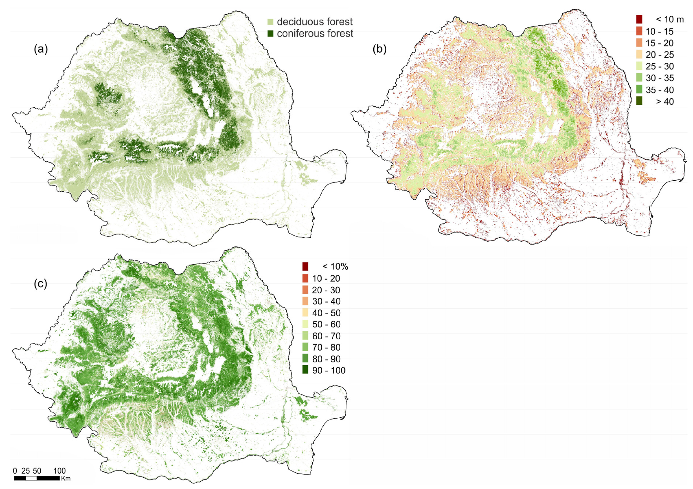
3.1. The Estimated AGFB in 2015. Transposing the Values into the Forest-Cover Map for 2006

Figure 6a shows the AGFB model for Romania, resulted by combining the allometric equation based on dbh with the estimated fd [47]. A total of 1259.8 Tg of AGFB, with an average of 150 Mg/ha⁻¹ and 4.18 Mg/tree, have been estimated for 2015. Among the dominated forest species, a total of 975.8 Tg (76.8% of the total AGFB) resulted, with an average of 151.5 Mg/ha⁻¹ and 4.36 Mg/tree for the deciduous forests, and a total of 284.0 Tg (23.2% of the total AGFB) with an average of 162.2 Mg/ha⁻¹ and 3.38 Mg/tree for the coniferous forests.

Regionally, significant differences were recorded for the major landform units (Figure 6b) and the major vegetation ecoregions (Figure 6c). The highest values were resulted for the Eastern Carpathians (471.10 Tg, 37.4% of the total), the Southern Carpathians (206.45 Tg, 16.4% of the total), the Apuseni Mountains (156.73 Tg, 12.4% of the total) and the Banat Mountains (129.65 Tg, 10.4% of the total). The lowest values were resulted for the Danube Delta and the Razim-Sinoie Lagoon Complex (0.18 Tg, <0.1% of the total), for the Banat and Crișana Plain (2.81 Tg, 0.2% of the total), the Dobrogea Plateau (5.57 Tg, 0.4% of the total) and the Romanian Plain (8.26 Tg, 0.7% of the total). However, by comparing the obtained quantity per ha, the highest AGFB values were resulted for the developed forests in the Banat Mountains (238.4 Mg/ha⁻¹) and the Southern Carpathians (204.6 Mg/ha⁻¹). For the Eastern Carpathians and Apuseni Mountains, a value of about 195 Mg/ha⁻¹ was obtained. The values that exceeds 100 Mg/ha⁻¹ were also estimated for the forests developed within the Subcarpathians (114.2 Mg/ha⁻¹) and Banat and Crișana Hills (103.5 Mg/ha⁻¹). The lowest values were estimated for the Danube Delta and the Razim-Sinoie Lagoon Complex (41.5 Mg/ha⁻¹), Banat and Crișana Plain (43.4 Mg/ha⁻¹) and for the Romanian Plain, the Moldavian Plateau and the Dobrogea Plateau (about 55 Mg/ha⁻¹).

The total estimated AGFB values significantly vary also according to the major vegetation ecoregions. Thus, the Carpathian montane coniferous forests comprise 721.6 Tg (57.3% of the total), Pannonian mixed forests 387.6 Tg (30.8% of the total), Central European mixed forests 107.4 Tg (8.5% of the total) and Balkan mixed forests 32.6 Tg (2.6% of the total). For the Pontic steppe and East European forest steppe a value of 6.2 Tg (0.5% of the total) and 4.3 Tg (0.3% of the total) respectively were resulted. As expected, the highest AGFB quantity per ha was obtained for the Carpathian montane coniferous forests (195.7 Mg/ha⁻¹) and Pannonian mixed forests (159.8 Mg/ha⁻¹), where the largest mountain forests area prevails. For the Central European mixed forests and Balkan mixed forests, values of 98.6 Mg/ha⁻¹ and 52.1 Mg/ha⁻¹, respectively have resulted. The reduced quantity obtained for the Pontic steppe (36.6 Mg/ha⁻¹) and East European forest steppe (30.5 Mg/ha⁻¹) reflects the lowest values of AGFB obtained for the forest-cover area developed in the Moldavian Plateau, Dobrogea Tableland, as well as in the Romanian Plain and Danube Delta.

By transposing the obtained AGFB values in 2015 to the forest-cover map in 2006, used as reference data to simulate future forest-cover change patterns, a difference of 7.47% has resulted. Specifically, a value of 1165.7 Tg was estimated for 2006, the resulting difference (−94.04 Tg) arising from different resolution and sources of the datasets used, as well as the resulting increase in the forest-cover area in the 2006–2015 period. Firstly, the effect of the different scales between the CLC dataset in 2006 (with a corresponding scale of about 1:100,000) and the derived data from Copernicus Land Monitoring Service for 2015 (with a resolution of 20 m) resulted in different details of the forest-cover pattern and, therefore, disagreements between the mapped area for these two years. Secondly, the interpolation procedure used to calculate AGFB for cells with unknown value may also influence the total AGFB amount estimated for 2006. In addition, the most consistent influence seems to arise from the resulting increase in the forest-cover area by 7.7% in the 2006–2015 period [43], as reflected in a lower total AGFB quantity for 2006 compared to 2015.

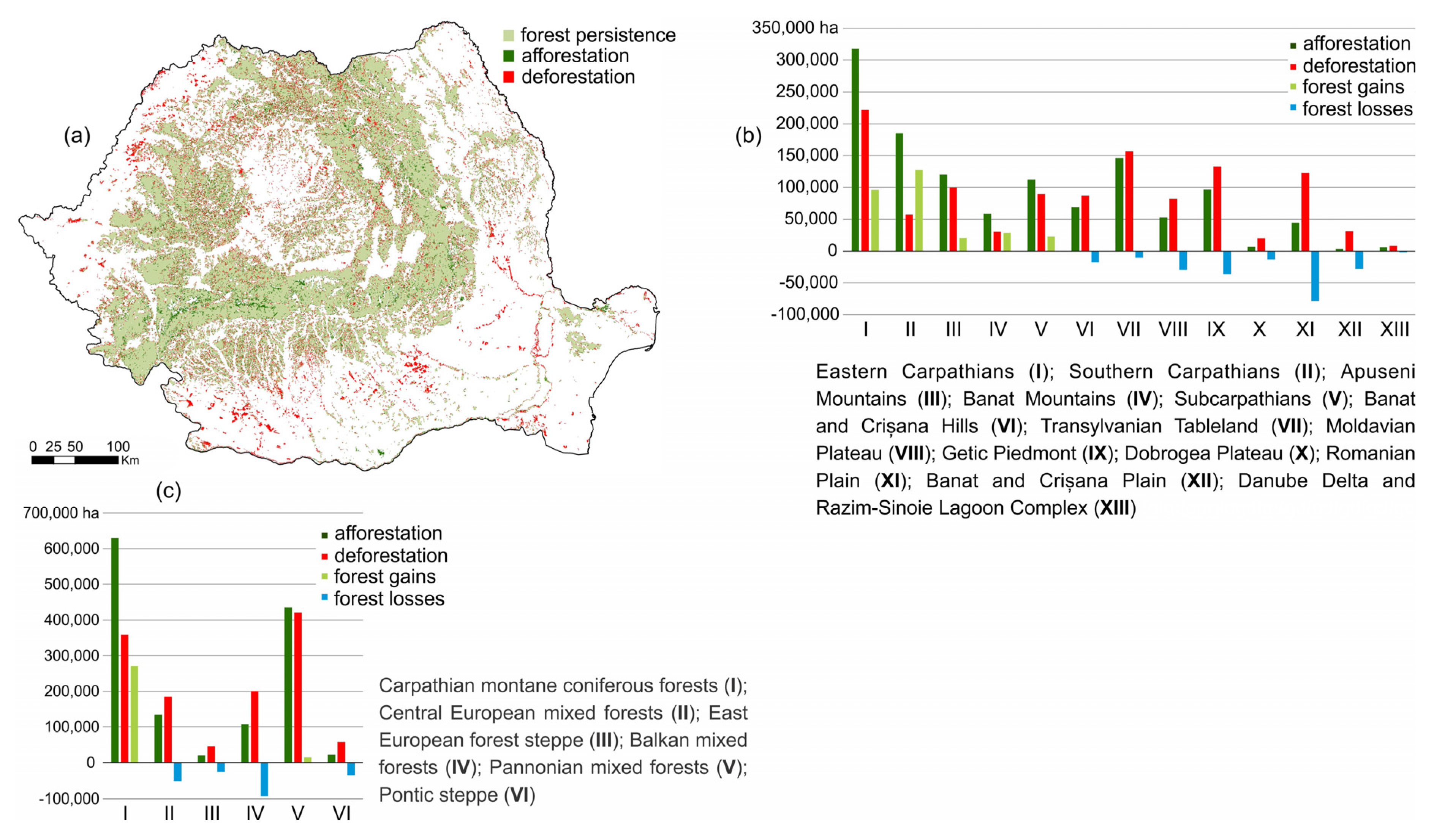
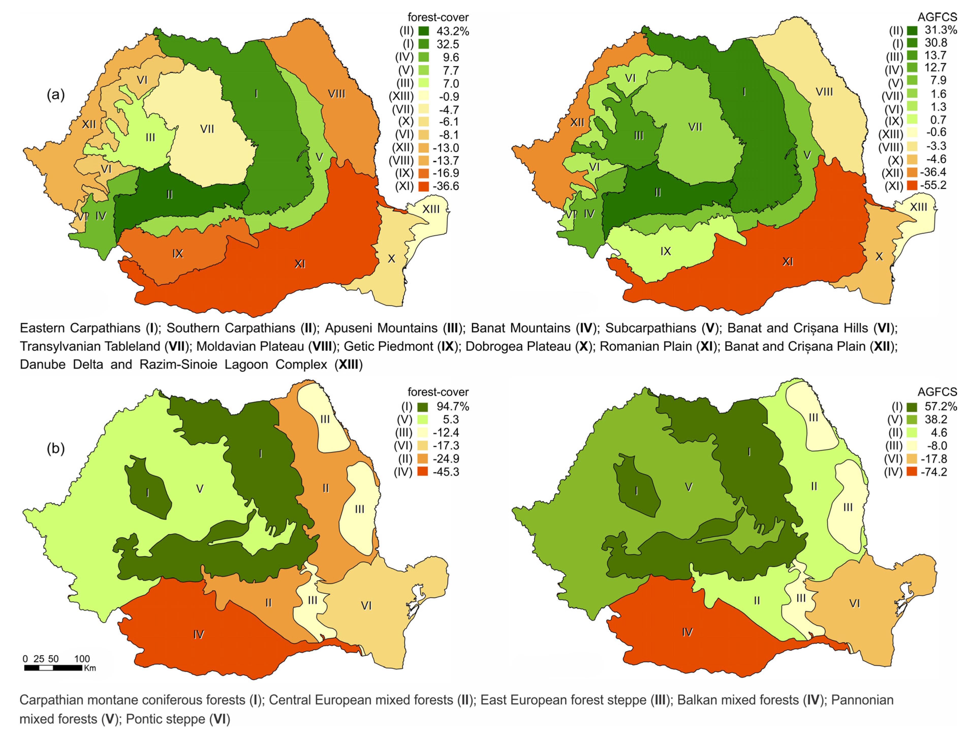
3.2. Predicted Forest-Cover Pattern Change

The simulation of the forest-cover pattern change [58] indicates large areas affected by forest gain and loss (Figure 7). Specifically, 1.207 mil. ha have been projected as the transition from non-forest categories to the forest category and 1.126 mil. ha as the transition from the forest category into non-forest categories. Overall, an increase of about 81,200 ha (1.2% of the total forest-cover area in 2006) was projected until 2050. Regionally, significant differences in forest-cover pattern change were resulted for the major relief units and the major vegetation ecoregions. Thus, according to the major landform units (Figure 7b), important forest gain was projected for the Southern Carpathians (127,800 ha, 43.2% of the total) and Eastern Carpathians (96,200 ha, 32.5% of the total). The positive trend of forest-cover area has also been projected for the Banat Mountains (28,550 ha, 9.6% of the total), the Subcarpathians (22,750 ha, 7.7% of the total) and the Apuseni Mountains (20,550 ha, 7.0% of the total). The highest values of forest loss were found in the Romanian Plain (78,400 ha, 36.6% of the total), the Getic Piedmont (36,300 ha, 16.9% of the total), the Moldavian Plateau (29,400 ha, 13.7% of the total) and the Banat and Crișana Plain (27,800 ha, 13.0% of the total).

When quantifying the major vegetation ecoregions (Figure 7c), almost all projected forest gain was identified in the Carpathian montane coniferous forests (94.7% of the total), where 629,700 ha simulated afforestation and 358,550 ha simulated deforestation have resulted in a positive balance of 271,100 ha. Forest gain was also projected for the Pannonian mixed forests (15,050 ha, 5.3% of the total). Forest loss was projected for the Balkan mixed forests (92,900 ha, 45.3% of the total), the Central European mixed forests (51,100 ha, 24.9% of the total), the Pontic steppe (35,500 ha, 17.3% of the total) and the East European forest steppe (25,450 ha, 12.4% of the total).

In terms of the simulated transition [58], results indicate the expansion of the forest-cover area mainly in relation to a decrease in pastures, natural grasslands and shrub association. The large forest loss was especially projected in relation to the expansion of agricultural lands (arable lands, heterogeneous agricultural areas and agricultural complex cultivation areas). Furthermore, locally, forest-cover loss is expected to be in relation to the expansion of built-up areas as the result of the urban growth process (mainly in the plain, tableland and plateau regions), as well as the development of tourist resorts (especially in the mountains regions).

The obtained K_Simulation values (>0) indicate that the CLUE-S model captured the trend in land-use/cover changes [86]. Specifically, the values higher than 0.6 resulting for the forest-cover, suggest that the model is fairly accurate. Furthermore, the K_Transition values (0.96–1.00) indicate that the allocation of transitions is almost totally correct, while the K_TransLoc values (0.70–1.00) indicate some errors caused by the incorrect amount of transitions.

However, the quantitative comparison of the observed and predicted change for 2006–2012 points to important errors in the simulated transitions [58], resulting in an underestimation of forest persistence by 5% and an overestimation of forest gain and forest loss by 14% and 41%, respectively. These errors can mainly be related to the limited number of determinant drivers included in the model and to the accuracy of the data used. On the one hand, the resulting pseudo R² [90] values, that range from 0.351 to 0.484, show that determinant factors included in the simulation regionally account for only 35.1% to 48.4% of the forest-cover pattern change [58]. This suggests that other factors (e.g., land-use planning, policies or projects; land tenure; climate change-related indicators; demographic and economic scenarios) may also explain the forest-cover pattern change in Romania [58]. On the other hand, the misclassification, the different classification schemes and the different resolutions associated with the CLC database [56,74,91] may lead to the uncertain quantification of historical forest-cover changes used to formulate the baseline scenario of the simulation.

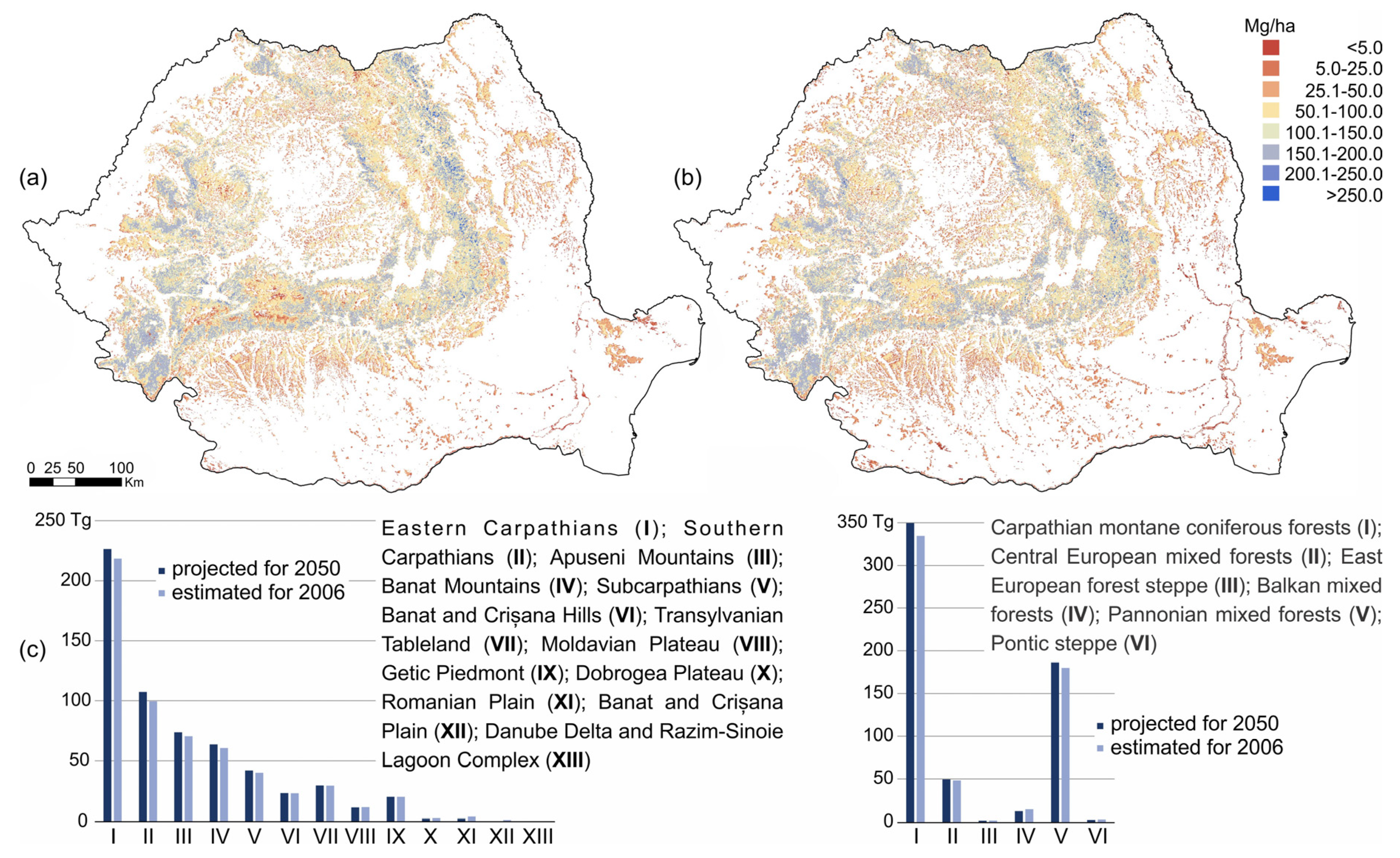
3.3. The Projected Potential Changes in AGFCS Quantity Up to 2050

According to the estimated AGFB values for 2006 and the projected forest-cover pattern change in 2050, the potential variations in AGFCS quantity were estimated for the 2006–2050 period. Thus, compared with the resulting AGFCS values in 2006 (Figure 8), an overall increase with approximately 23.43 Tg has resulted for 2050. The projected quantity significantly varies regionally, increasing in the Southern Carpathians (+8.12 Tg), the Eastern Carpathians (+7.99 Tg), the Apuseni Mountains (+3.54 Tg), the Banat Mountains (+3.30 Tg), the Subcarpathians (+2.05 Tg), the Transylvanian Tableland (+0.40 Tg), the Banat and Crișana Hills (+0.33 Tg) and the Getic Piedmont (+0.19 Tg). The model estimated a drop in the Romanian Plain (−1.37 Tg), in the Banat and Crișana Plain (−0.91 Tg), the Dobrogea Plateau (−0.11 Tg), the Moldavian Plateau (−0.08 Tg) and the Danube Delta and the Razim-Sinoie Lagoon Complex (−0.01 Tg). In accordance with the major vegetation ecoregions, the results suggest a rise in the Carpathian montane coniferous forests (+15.14 Tg), in the Pannonian mixed forests (+10.10 Tg) and the Central European mixed forests (+1.21 Tg) and a drop in the Balkan mixed forests (−2.24 Tg), the Pontic steppe (−0.54 Tg) and the East European forest steppe (−0.24 Tg).

When quantifying the variation of AGFCS in relation to the projected forest-cover dynamics, there resulted significant differences between the forest-cover gain/loss and the corresponding increases/decreases in AGFCS quantity (Figure 9). Accordingly, the projected forest gain in the Southern Carpathians (43.2% of the total), the Eastern Carpathians (32.5% of the total), the Banat Mountains (9.6% of the total), the Subcarpathians (7.7% of the total) and the Apuseni Mountains (6.9% of the total) resulted in a corresponding AGFCS increase by 31.3% in the Southern Carpathians, 30.8% in the Eastern Carpathians, 13.7% in the Apuseni Mountains 12.7% in the Banat Mountains and 7.9% in the Subcarpathians. The total projected forest loss (36.6% in the Romanian Plain, 13.7% in the Moldavian Plateau, 13.0% in the Banat and Crișana Plain, 6.1% in the Dobrogea Plateau and 0.9% in the Danube Delta and Razim-Sinoie Lagoon Complex) has resulted in AGFCS decreases by 55.2% in the Romanian Plain, 36.4% in the Banat and Crișana Plain and <5% in the Dobrogea and Moldavian Plateaus and the Danube Delta and Razim-Sinoie Lagoon Complex. However, the resulting forest loss in the Getic Piedmont (16.9% of the total), the Banat and Crișana Hills (8.1% of the total) and the Transylvanian Tableland (4.7% of the total) has resulted in AGFCS increases by 0.7%, 1.3% and 1.6%, respectively.

In terms of major vegetation ecoregions, the total projected forest gain in the Carpathian montane coniferous forests (94.7% of the total) and Pannonian mixed forests (5.3% of the total) has resulted in a percentage of 95.4% of the total AGFCS increases: 57.2% in the Carpathian montane coniferous forests and 38.2% in the Pannonian mixed forests. The projected forest loss in the Balkan mixed forests (45.4% of the total), the Pontic steppe (17.3% of the total) and the East European forest steppe (12.4% of the total) has resulted in a drop in AGFCS by 74.2%, 17.8% and 7.9%, respectively. However, the projected forest loss in the Central European mixed forests (24.9% of the total) has resulted in 4.6% of the total AGFCS increases.

4. Discussion

The baseline AGFB model used in the present approach overestimates the total quantity by about 17% compared to the estimated amount reported in the FAO’s Global Forest Resource Assessment [43] and the Executive Report of the European Map of Living Forest Biomass and Carbon Stock [10]. An overestimation (11%) was also found compared to the estimated amount reported in the “Use of National Forest Inventories data to estimate the biomass in the European Forests”—Final report [92]. Furthermore, converting the total standing wood volume (m³) estimated by [93] to tons by using the mean conversion figure 1 m³ = 725 kg [94], our overestimates increase to 22.3% for the all estimated amount, and to 4.7% for the estimated quantity per ha. By comparing the resulting values for the dominant forest species [93], the AGFB model exceeds by 34.6% the estimated quantity for deciduous species, but is inferior by 10.4% for coniferous species. Additionally, according to the estimated value for beech forests [95], our results underestimate the AGFB quantity for deciduous species by 32%. However, these AGFB data provided by different sources are not directly comparable because they use different approaches to estimate tree biomass, different allometric indicators, different sampling designs, different specific time-period and different definitions for forest vegetation over the study area.

Overall, according to the AGFB model used, a total of 629.9 Tg of AGFCS quantity was resulted for 2015, thus making up 6.3% of the total estimated carbon stock in forest biomass in EU countries [96]. By integrating the AGFB model and forest-cover pattern change scenario, our findings suggest a potential increase in AGFCS in the near future, the calculated positive trend (+4.02%) at national scale resulting from the potential increase of AGFB with 46.86 Tg. However, as presented in Section 3.3, we found that the variation of the AGFCS amount is not directly related to the projected forest-cover pattern dynamics across the area, the resulting correspondence reflecting significant a regional and local variation of the forest indicators used to estimate AGFB values. For example, the resulting increases of AGFCS in the Getic Piedmont, the Banat and Crișana Hills and the Transylvanian Tableland in relation to the projected forest loss can indicate that the projected afforestation will prevail in the consistent forest areas, characterized by high allometric values, while deforestation will be prevalent in the forest areas with low allometric values and density. Furthermore, the estimated increases of AGFCS in the Central European mixed forests ecoregion, where significant forest loss was projected, seems to result from the high AGFB values calculated for the hilly area (where predominantly afforestation was projected) and low AGFB values calculated for the plain, tableland and plateau areas (where mainly forest loss is projected).

Due to its large expansion, forest vegetation represents the most important biomass resource in Romania. However, varying biophysical and socio-economic conditions, as well as historical and current land-use changes, are seen in significant regional forest-cover variations [74] and thus, in the important regional variation of AGFB in the area. In this regard, our results support the idea that the projected disparities in the forest-cover pattern change will result in a large variation of aboveground forest carbon sink in the area, with net differences between the analyzed major landform units and major vegetation ecoregions. Overall, the projected increase of forest-cover area in the mountainous and hilly regions is expected to result in a potential gain of about 23.43 Tg of AGFCS by 2050. In contrast, the considerable decrease in forest-cover area projected for the tableland, plateau and plain regions is expected to result in the significant loss of approximately 2.3 Tg. Accordingly, our results suggest that expected forest-cover change can compromise carbon storage, which can have important environmental implications. On the one hand, this can accentuate the effects of climate variability and change and therefore, lead to the increase of socio-economic vulnerability to drought in the area [97], given that these regions integrate most of the largest towns in Romania and the highest population density (approximatively 132 inhabitants/km²) [98]. On the other hand, these changes can increase the risk of drought and desertification having an impact on the agricultural systems [99,100] and groundwater processes [58].

Due to the important role of forest biomass in climate change mitigation and adaptation strategies [5], our results may be significant in implementing effective sustainable forest management options and related policies. However, the resulting difference between our AGFB model and other estimated values for Romania suggests that this baseline data may contain several spatial errors of quantity and allocation and therefore, represent an uncertainty for the practical management of applications and decisions [101].

Furthermore, the predictive attribute of the data referring to the potential variation of the AGFCS quantity can have important implications for managing carbon in the forest sector by estimating potential emissions in relation to the forest gain and loss. In addition, the resulting spatially-explicit maps can provide baseline information for assessing the value of forest ecosystem goods and services at pan-European level [10], but also to estimate the potential changes that may occur in the near future. However, predicting the variation of the AGFCS without modeling the potential changes in forest structure and composition recommend that the obtained results must first be considered as indicating the potential trend at national and regional scale, whereas the resulting changes at local level must be interpreted carefully.

5. Conclusions

The present study attempted to estimate future potential variation of aboveground forest carbon stock in Romania, by integrating into the spatial and statistical analysis the estimated aboveground forest biomass for 2015 and the forest-cover pattern change scenario simulated for 2050. Our findings indicate an overall increase trend in aboveground forest carbon stock up to 2050 at the national scale, suggesting that the changes in the forest-cover pattern in the area can significantly affect the quantity of aboveground forest biomass over time. Specifically, the simulated changes in forest-cover pattern show an overall gain of aboveground forest carbon stock (+4%), as the result of the increased biomass (+58.85 Tg) estimated for the forest vegetation mainly occurring in the mountain regions and the decreased biomass (−4.98 Tg) estimated for the forest vegetation developed mainly in the plain areas.

Considering the uncertainties that have affected the resulting data, we assume that several spatial errors may influence the accuracy of our estimation and therefore, the methodology presented can be further refined. Hence, using spatial models of potential changes in forest structure and composition over time may improve the current approach towards obtaining better and more practical results. However, this work may prove to be an essential step towards understanding the potential impact of future forest disturbances on the forest carbon sink and therefore, could provide better perspectives in terms of forest policy and environmental decision-making. Additionally, the current study could be the starting point for future works aimed at assessing the impact of land-use/cover change on carbon stock by incorporating the methodology presented.

References

1. Hofmann, D.J.; Butler, J.H.; Dlugokencky, E.J.; Elkins, J.W.; Masarie, K.; Montzka, S.A.; Tans, P. The role of carbon dioxide in climate forcing from 1979 to 2004: Introduction of the Annual Greenhouse Gas Index. Tellus 2006, 58B, 614–619. [Google Scholar] [CrossRef]
2. Dixon, R.K.; Brown, S.; Houghton, R.A. Carbon pools and flux of global forest ecosystems. Science 1994, 263, 185–190. [Google Scholar] [CrossRef] [PubMed]
3. Field, C.; Lobell, D.B.; Peters, H.A.; Chiariello, N.R. Feedbacks of Terrestrial Ecosystems to Climate Change. Annu. Rev. Environ. Resour. 2007, 32, 29. [Google Scholar] [CrossRef] [Green Version]
4. Teobaldelli, M.; Somogyi, Z.; Migliavacca, M.; Usoltsev, V.A. Generalized functions of biomass expansion factors for conifers and broadleaved by stand age, growing stock and site index. For. Ecol. Manag. 2009, 257, 1004–1013. [Google Scholar] [CrossRef]
5. Kumar, R.; Nandy, S.; Agarwal, R.; Kushwaha, S.P.S. Forest cover dynamics analysis and prediction modeling using logistic regression model. Ecol. Indic. 2014, 45, 444–455. [Google Scholar] [CrossRef]
6. Brown, S.; Sathaye, J.; Cannell, M.; Kauppi, P.E. Mitigation of carbon emission to the atmosphere by forest management. Commonw. For. Rev. 1996, 75, 80–91. [Google Scholar]
7. Zianis, D.; Muukkonen, P.; Mäkipää, R.; Mencuccini, M. Biomass and Stem Volume Equations for Tree Species in Europe, Silva Fennica Monographs 4; The Finnish Society of Forest Science: Tampere, Finland, 2005. [Google Scholar]
8. Cairns, M.A.; Brown, S.; Helmer, E.H.; Baumgardner, G.A. Root biomass allocation in the world’s upland forests. Oecologia 1997, 111, 1–11. [Google Scholar] [CrossRef]
9. Bi, H.; Turner, J.; Lambert, M.J. Additive biomass equations for native eucalypt forest trees of temperate Australia. Trees-Struct. Funct. 2004, 18, 467–479. [Google Scholar] [CrossRef]
10. Barredo, J.I.; Miguel, J.S.; Caudullo, G.; Busetto, L. A European Map of Living Forest Biomass and Carbon Stock. Executive Report; Joint Research Centre of the European Commission: Ispra, Italy, 2012. [Google Scholar] [CrossRef]
11. Houghton, R.; Hall, F.; Goetz, S. Importance of biomass in the global carbon cycle. J. Geophys. Res. Biogeosci. 2009, 114, G2. [Google Scholar] [CrossRef]
12. Climate Change. The IPCC Scientific Assessment; Houghton, J.T.; Jenkins, G.J.; Ephraums, J.J. (Eds.) Cambridge University Press: Cambridge, UK, 1990. [Google Scholar]
13. Lamlom, S.H.; Savidge, R.A. A reassessment of carbon content in wood: Variation within and between 41 North American species. Biomass Bioenergy 2003, 25, 381–388. [Google Scholar] [CrossRef]
14. CEOS Land Product Validation Subgroup. Available online: https://lpvs.gsfc.nasa.gov/Biomass/AGB_home.html (accessed on 16 June 2020).
15. Wilkes, P.; Disney, M.; Vicari, M.B.; Calders, K.; Burt, A. Estimating urban above ground biomass with multi-scale LiDAR. Carbon Balance Manag. 2018, 13, 10. [Google Scholar] [CrossRef] [PubMed]
16. Basuki, T.M.; Skidmore, A.K.; van Laake, P.E.; van Duren, I.; Hussin, Y.A. The Potential of Spectral Mixture Analysis to Improve the Estimation Accuracy of Tropical Forest Biomass. Geocarto Int. 2012, 27, 329–345. [Google Scholar] [CrossRef]
17. Brown, S. Estimating Biomass and Biomass Change of Tropical Forests: A Primer; FAO Forestry Paper; Food and Agriculture Organization of the United Nations: Rome, Italy, 1997; Volume 134, p. 55. [Google Scholar]
18. Brown, S. Measuring carbon in forests: Current status and future challenges. Environ. Pollut. 2002, 116, 363–372. [Google Scholar] [CrossRef]
19. Somogyi, Z.; Cienciala, E.; Makipaa, R.; Muukkonen, P.; Lehtonen, A.; Weiss, P. Indirect methods of largescale forest biomass estimation. Eur. J. Res. 2007, 126, 197–207. [Google Scholar] [CrossRef]
20. Myneni, R.B.; Hall, F.G.; Sellers, P.J.; Marshak, A.L. The interpretation of spectral vegetation indexes. IEEE Trans. Geosci. Remote Sens. 1995, 33, 481–486. [Google Scholar] [CrossRef]
21. Dong, J.R.; Kaufmann, R.K.; Myneni, R.B.; Tucker, C.J.; Kauppi, P.E.; Liski, J.; Buermann, W.; Alexeyev, V.; Hughes, M.K. Remote sensing estimates of boreal and temperate forest woody biomass: Carbon pools, sources and sinks. Remote Sens. Environ. 2003, 84, 393–410. [Google Scholar] [CrossRef] [Green Version]
22. Calders, K.; Raumonen, P.; Herold, M. Nondestructive estimates of above-ground biomass using terrestrial laser scanning. Methods Ecol. Evol. 2015, 6, 198–208. [Google Scholar] [CrossRef]
23. Dassot, M.; Colin, A.; Santenoise, P.; Fournier, M.; Constant, T. Terrestrial laser scanning for measuring the solid wood volume, including branches, of adult standing trees in the forest environment. Comput. Electron. Agric. 2012, 89, 86–93. [Google Scholar] [CrossRef]
24. Ferraz, A.; Saatchi, S.; Mallet, C.; Meyer, V. Lidar Detection of Individual Tree Size in Tropical Forests. Remote Sens. Environ. 2016, 183, 318–333. [Google Scholar] [CrossRef]
25. Mohd Zaki, N.A.; Abd Latif, Z.; Suratman, M.N.; Zainal, M.Z. Aboveground Biomass and Carbon Stocks Modelling using Non-Linear Regression Model. In IOP Conference Series: Earth and Environmental Science; IOP Publishing: Bristol, UK, 2016; Volume 37. [Google Scholar] [CrossRef]
26. Goetz, S.J.; Baccini, A.; Laporte, N.T.; Johns, T.; Walker, W.; Kellndorfer, J.; Houghton, R.A.; Sun, M. Mapping and monitoring carbon stocks with satellite observations: A comparison of methods. Carbon Balance Manag. 2009, 4, 2. [Google Scholar] [CrossRef] [Green Version]
27. Zianis, D.; Mencuccini, M. On simplifying allometric analyses of forest biomass. For. Ecol. Manag. 2004, 187, 311–332. [Google Scholar] [CrossRef]
28. Ter-Mikaelian, M.T.; Korzukhin, M.D. Biomass equations for sixty-five North American tree species. For. Ecol. Manag. 1997, 97, 1–24. [Google Scholar] [CrossRef] [Green Version]
29. Schmitt, M.D.C.; Grigal, D.F. Generalized biomass estimation equation for Betula papyrifera Marsh. Can. J. For. Res. 1981, 11, 837–840. [Google Scholar] [CrossRef]
30. Wirth, C.; Schumacher, J.; Schulze, E.-D. Generic biomass functions for Norway spruce in central Europe—A metaanalysis approach toward prediction and uncertainty estimation. Tree Physiol. 2004, 24, 121–139. [Google Scholar] [CrossRef] [Green Version]
31. Duncanson, L.; Huang, W.; Johnson, K.; Swatantran, A.; McRoberts, R.E.; Dubayah, R. Implications of allometric model selection for county-level biomass mapping. Carbon Balance Manag. 2017, 12, 18. [Google Scholar] [CrossRef]
32. Chave, J.; Réjou-Méchain, M.; Búrquez, A.; Chidumayo, E.; Colgan, M.S.; Delitti, W.B.; Duque, A.; Eid, T.; Fearnside, P.M.; Goodman, R.C.; et al. Improved allometric models to estimate the aboveground biomass of tropical trees. Glob. Chang. Biol. 2014, 20, 3177–3190. [Google Scholar] [CrossRef]
33. Vashum, K.T.; Jayakumar, S. Methods to Estimate Above-Ground Biomass and Carbon Stock in Natural Forests—A Review. J. Ecosyst. Ecogr. 2012, 2. [Google Scholar] [CrossRef]
34. Tan, K.; Piao, S.; Peng, C.; Fang, J. Satellite-based estimation of biomass carbon stocks for northeast China’s forests between 1982 and 1999. For. Ecol. Manag. 2007, 240, 114–121. [Google Scholar] [CrossRef]
35. Avitabile, V.; Herold, M.; Heuvelink, G.B.M.; Lewis, S.L.; Phillips, O.L.; Asner, G.P.; Armston, J.; Ashton, P.S.; Banin, L.; Bayol, N.; et al. An integrated pan-tropical biomass map using multiple reference datasets. Glob. Chang. Biol. 2016, 22, 1406–1420. [Google Scholar] [CrossRef] [Green Version]
36. Avitabile, V.; Camia, A. An assessment of forest biomass maps in Europe using harmonized national statistics and inventory plots. For. Ecol. Manag. 2018, 409, 489–498. [Google Scholar] [CrossRef]
37. Cartus, O.; Kellndorfer, J.; Walker, W.; Bishop, J.; Franco, C.; Santos, L.; Michel Fuentes, J.M. A national, detailed map of forest aboveground carbon stocks in Mexico. Remote Sens. 2014, 6, 5559–5588. [Google Scholar] [CrossRef] [Green Version]
38. Dubayah, R.O.; Sheldon, S.L.; Clark, D.B.; Hofton, M.A.; Blair, J.B.; Hurtt, G.C.; Chazdon, R.L. Estimation of tropical forest height and biomass dynamics using lidar remote sensing at La Selva, Costa Rica. J. Geophys. Res. 2010, 15, 1–17. [Google Scholar]
39. Rodríguez-Veiga, P.; Saatchi, S.; Tansey, K.; Balzter, H. Magnitude, spatial distribution and uncertainty of forest biomass stocks in Mexico. Remote Sens. Environ. 2016, 183, 265–281. [Google Scholar] [CrossRef] [Green Version]
40. Saatchi, S.S.; Harris, N.L.; Brown, S.; Lefsky, M.; Mitchard, E.T.; Salas, W.; Zutta, B.R.; Buermann, W.; Lewis, S.L.; Hagen, S.; et al. Benchmark map of forest carbon stocks in tropical regions across three continents. Proc. Natl. Acad. Sci. USA 2011, 108, 9899–9904. [Google Scholar] [CrossRef] [PubMed] [Green Version]
41. Brovkina, O.; Novotny, J.; Cienciala, E.; Zemek, F.; Russ, R. Mapping forest aboveground biomass using airborne hyperspectral and LiDAR data in the mountainous conditions of Central Europe. Ecol. Eng. 2017, 100, 219–230. [Google Scholar] [CrossRef]
42. Muukkonen, P. Generalized allometric volume and biomass equations for some tree species in Europe. Eur. J. For. Res. 2007, 126, 157–166. [Google Scholar] [CrossRef]
43. FRA (Global Forest Resources Assessment). Global Forest Resources Assessment 2015; Desk Reference; Food and Agriculture Organization of the United Nations: Rome, Italy, 2015. [Google Scholar]
44. Blujdea, V.N.B.; Pilli, R.; Dutca, I.; Ciuvat, L.; Abrudan, I.V. Allometric biomass equations for young broadleaved trees in plantations in Romania. For. Ecol. Manag. 2012, 264, 172–184. [Google Scholar] [CrossRef]
45. Dutcă, I.; Abrudan, I.V.; Stăncioiu, P.T.; Blujdea, V. Biomass conversion and expansion factors for young Norway Spruce (Picea abies (L.) Karst) trees planted on non-forest lands in Romania. NBHA 2010, 38, 286–292. [Google Scholar]
46. Stancioiu, P.T.; O’Hara, K.L. Leaf area and growth efficiency of regeneration in mixed species, multiaged forests of the Romanian Carpathians. For. Ecol. Manag. 2006, 222, 55–66. [Google Scholar] [CrossRef]
47. Kucsicsa, G.; Dumitrică, C.; Dumitrașcu, M.; Grigorescu, I.; Vrînceanu, A. Estimation of Above-Ground Forest Biomass in Romania, Ecological and Geographical Problems of Transition to a Green Economy in the Countries and Regions of the CIS; Conference Book: Minsk, Belarus, 2019; pp. 145–151. [Google Scholar]
48. Le Page, Y.; Hurtt, G.; Thomson, A.M.; Bond-Lamberty, B.; Patel, P.; Wise, M.; Calvin, K.V.; Kyle, P.; Clarke, L.; Edmonds, J.; et al. Sensitivity of climate mitigation strategies to natural disturbances. Environ. Res. Lett. 2013, 8, 1–6. [Google Scholar] [CrossRef]
49. Lambin, E.F. Modelling Deforestation Processes, A Review; EUR 15744 EN, TREES Series B: Research Report No. 1; Joint Research Centre, Institute for Remote Sensing Applications: Ispra, Italy; European Space Agency, Luxembourg, Office for Official Publications of the European Community: Luxembourg, 1994; p. 128. [Google Scholar]
50. Veldkamp, A.; Fresco, L.O. CLUE: A conceptualmodel to study the conversion of land use and its effects. Ecol. Model. 1996, 85, 253–270. [Google Scholar] [CrossRef]
51. Verburg, P.H.; Veldkamp, A. Projecting land use transitions at forest fringes in the Philippines at two spatial scales. Landsc. Ecol. 2004, 19, 77–98. [Google Scholar] [CrossRef]
52. Forest Europe. UNECE. FAO. State of Europe’s Forests 2011. Status and Trends in Sustainable Forest Management in Europe; Ministerial Conference on the Protection of Forests in Europe, Liaison Unit Oslo: Zvolen, Slovakia, 2011. [Google Scholar]
53. Griffiths, P.; Kuemmerle, T.; Kennedy, R.E.; Abrudan, I.V.; Knorn, J.; Hostert, P. Using annual time-series of Landsat images to assess the effects of forest restitution in postsocialist Romania. Remote Sens. Environ. 2012, 118, 199–214. [Google Scholar] [CrossRef]
54. Hanganu, J.; Constantinescu, A. Land cover changes in Romania based on Corine land cover inventory 1990–2012. Rev. Roum. Géogr. Rom. J. Geogr. 2015, 59, 111–116. [Google Scholar]
55. Kucsicsa, G.; Popovici, E.-A.; Bălteanu, D.; Grigorescu, I.; Dumitrașcu, M.; Mitrică, B. Future land use/cover changes in Romania: Regional simulations based on CLUE-S model and CORINE land cover database. Landsc. Ecol. Eng. 2019, 15, 75–90. [Google Scholar] [CrossRef]
56. Petrişor, A.I. Using CORINE data to look at deforestation in Romania: Distribution & possible consequences. Urbanism 2015, 6, 83–90. [Google Scholar]
57. Popovici, E.-A.; Bălteanu, D.; Kucsicsa, G. Assessment of changes in Land–Use and Land–Cover pattern in Romania using Corine Land Cover database. Carpathian J. Earth Environ. Sci. 2013, 8, 195–208. [Google Scholar]
58. Kucsicsa, G.; Popovici, A.-E.; Bălteanu, D.; Dumitrașcu, M.; Grigorescu, I.; Mitrică, B. Assessing the potential future forest cover change in Romania, predicted using scenario-based modelling. Environ. Model. Assess. 2019, 1–21. [Google Scholar] [CrossRef]
59. Bălteanu, D.; Popovici, E.A. Land use changes and land degradation in post–socialist Romania. Rev. Roum. Géogr. Rom. J. Geogr. 2010, 54, 95–105. [Google Scholar]
60. European Environmental Agency (EEA). Copernicus Land Monitoring Service—CORINE Land Cover 2006. Available online: https://land.copernicus.eu/pan-european/corine-land-cover/clc-2006 (accessed on 12 February 2019).
61. European Environment Agency. DMEER: Digital Map of European Ecological Regions. 2003. Available online: https://www.eea.europa.eu/data-and-maps/data/digital-map-of-european-ecological-regions (accessed on 17 June 2019).
62. NIS (National Institute of Statistics). Romanian Statistical Yearbook; National Institute of Statistics: Bucharest, Romania, 2019; p. 711. [Google Scholar]
63. Gurung, A.B.; Bokwa, A.; Chełmicki, W.; Elbakidze, M.; Hirschmugl, M.; Hostert, P.; Ibisch, P.; Kozak, J.; Kuemmerle, T.; Matei, E.; et al. Global change research in the Carpathian Mountain region. Mt. Res. Dev. 2009, 29, 282–288. [Google Scholar] [CrossRef] [Green Version]
64. Veen, P.; Fanta, J.; Raev, I.; Biris, I.-A.; de Smidt, J.; Maes, B. Virgin forests in Romania and Bulgaria: Results of two national inventory projects and their implications for protection. Biodivers. Conserv. 2010, 19, 1805–1819. [Google Scholar] [CrossRef]
65. Geacu, S.; Dumitrașcu, M.; Maxim, I. The evolution of the natural protected areas network in Romania. Rev. Rom. Géogr. Rom. J. Geogr. 2012, 56, 33–41. [Google Scholar]
66. Abrudan, I.V.; Marinescu, V.; Ionescu, O.; Ioras, F.; Horodnic, S.A.; Sestras, R. Developments in the Romanian Forestry and its Linkages with other Sectors. Not. Bot. Horti Agrobot. Cluj-Napoca 2009, 37, 14–21. [Google Scholar] [CrossRef] [Green Version]
67. Strimbu, B.M.; Hickey, G.M.; Strimbu, V.G. Forest conditions and management under rapid legislation change in Romania. For. Chron. 2005, 81, 350–358. [Google Scholar] [CrossRef]
68. Kissling-Näf, I.; Bisang, K. Rethinking recent changes of forest regimes in Europe through property-rights theory and policy analysis. For. Policy Econ. 2001, 3, 99–111. [Google Scholar] [CrossRef]
69. Lerman, Z.; Csaki, C.; Feder, G. Evolving farm structures and land-use patterns in former socialist countries. Q. J. Int. Agric. 2004, 43, 309–335. [Google Scholar]
70. Turnock, D. Ecoregion-based conservation in the Carpathians and the land use implications. Land Use Policy 2002, 19, 47–63. [Google Scholar] [CrossRef]
71. Bălteanu, D.; Felciuc, M.; Dumitraşcu, M.; Grigorescu, I. Environmental changes in the Maramureş Mountains Natural Park. In Sustainable Development in Mountain Regions, Southestern Europe; Zhelezov, G., Ed.; Springer International Publishing: Cham, Switzerland, 2016; pp. 335–348. Available online: http://link.springer.com/book/10.1007/978-3-319-20110-8 (accessed on 24 April 2018). [CrossRef]
72. Griffiths, P.; Müller, D.; Kuemmerle, T.; Hostert, P. Agricultural land change in the Carpathian ecoregion after the breakdown of socialism and expansion of the European Union. Environ. Res. Lett. 2013, 8. [Google Scholar] [CrossRef]
73. Munteanu, C.; Kuemmerle, T.; Boltižiar, M.; Butsic, V.; Gimmi, U.; Halada, L.; Kaim, D.; Király, G.; Konkoly-Gyuró, É.; Kozak, J.; et al. Forest and agricultural land change in the Carpathian region—A metaanalysis of long-term patterns and drivers of change. Land Use Policy 2014, 38, 685–697. [Google Scholar] [CrossRef]
74. Kucsicsa, G.; Dumitrică, C. Spatial modelling of deforestation in Romanian Carpathian Mountains using GIS and Logistic Regression. J. Mt. Sci. 2019, 16, 1005–1022. [Google Scholar] [CrossRef]
75. Knorn, J.; Kuemmerle, T.; Radeloff, V.C.; Szabo, A.; Mîndrescu, M.; Keeton, W.S.; Abrudan, I.; Griffiths, P.; Gancz, V.; Hostert, P. Forest restitution and protected area effectiveness in post-socialist Romania. Biol. Conserv. 2012, 146, 204–212. [Google Scholar] [CrossRef]
76. Dutcă, I.; Abrudan, I.V. Estimation of forest land–cover change in Romania, between 1990 and 2006. Bull. Transilv. Univ. Bras. 2010, 3, 33–36. [Google Scholar]
77. Kucsicsa, G.; Bălteanu, D. The influence of man-induced land-use change on the upper forest limit in the Romanian Carpathians. Eur. J. For. Res. 2020. [Google Scholar] [CrossRef]
78. Posea, G.; Badea, L. România, Harta Unităţilor de Relief (Regionarea Geomorfologică). Ed; Ştiinţifică şi Enciclopedică: Bucharest, Romania, 1984. [Google Scholar]
79. Marklund, L.G. Biomass functions for Norway spruce (Picea abies (L.) Karst.) in Sweden. Rapp. -Sver. Lantbr. Inst. foer Skogstaxering (Sweden) 1987, 43, 1–127. [Google Scholar]
80. Marklund, L.G. Biomassafunktioner for tall, gran och björk i Sverige. Sveriges lantbruksuniversitet. Inst. för skogstaxering 1988, 45, 1–73. [Google Scholar]
81. Pastor, J.; Aber, J.D.; Melillo, J.M. Biomass prediction using generalized allometric regressions for some northeast tree species. For. Ecol. Manag. 1984, 7, 265–274. [Google Scholar] [CrossRef]
82. Näslund, M. Skogsförsöksanstaltens Gallringsförsök i Tallskog. Meddelanden Från Statens Skogsförsökanstalt; Bsselte ab.: Stockholm, Sweden, 1937; Volume 29, pp. 1–169. [Google Scholar]
83. Verburg, P.H.; Soepboer, W.; Limpiada, R.; Espaldon, M.V.O.; Sharifa, M.; Veldkamp, A. Land use change modelling at the regional scale: The CLUE–S model. Environ. Manag. 2002, 30, 391–405. [Google Scholar] [CrossRef]
84. Menard, S. Applied Logistic Regression Analysis, 2nd ed.; Series: Quantitative Applications in the Social Sciences; Sage Publications: London, UK, 2002. [Google Scholar]
85. Verburg, P.H.; Overmars, K.P. Combining top–down and bottom–up dynamics in land use modeling: Exploring the future of abandoned farmlands in Europe with the Dyna–CLUE model. Landsc. Ecol. 2009, 24, 1167–1181. [Google Scholar] [CrossRef]
86. van Vliet, J.; Bregtb, A.K.; Hagen-Zankerc, A. Revisiting Kappa to account for change in the accuracy assessment of land-use change models. Ecol. Model. 2011, 222, 1367–1375. [Google Scholar] [CrossRef]
87. Cohen, J. A coefficient of agreement for nominal scale. Educ. Psychol. Meas. 1960, 20, 37–46. [Google Scholar] [CrossRef]
88. Philip, G.M.; Watson, D.F. A Precise Method for Determining Contoured Surfaces. APPEA J. 1982, 22, 205–212. [Google Scholar] [CrossRef]
89. Weber, D.D.; Englund, E.J. Evaluation and comparison of spatial interpolators II. Math. Geol. 1984, 26, 589–603. [Google Scholar] [CrossRef]
90. Nagelkerke, N.J.D. A note on a general definition of the coefficient of determination. Biometrika 1991, 78, 691–692. [Google Scholar] [CrossRef]
91. Popovici, E.-A.; Kucsicsa, G.; Bălteanu, D.; Grigorescu, I.; Mitrică, B.; Dumitrașcu, M.; Damian, N. Past and future land use/cover flows related to agricultural lands in Romania. An assessment using CLUE-S Model and CORINE Land Cover Database. Carpathian J. Earth Environ. Sci. 2018, 13, 613–628. [Google Scholar] [CrossRef]
92. Henning, L.; Korhonen, K.T.; Lanz, A.; Riedel, T. Final Report, Specific Contract n. 17 “Use of National Forest Inventories Data to Estimate Biomass in the European Forests” in the Context of the “Framework Contract for the Provision of Forest Data and Services in Support to the European Forest Data Centre”, 15 April 2016; Joint Research Centre of the European Commission: Ispra, Italy, 2016. [Google Scholar]
93. Scarlat, N.; Blujdea, V.N.; Dallemand, J.-F. Assessment of the availability of agricultural and forest residues for bioenergy production in Romania. Biomass Bioenergy 2011, 35, 1995–2005. [Google Scholar] [CrossRef]
94. Rosillo-Calle, F.; Furdato, P.; Rezende, M.E.A.; Hall, D.O. The Charcoal Dilemma: Finfing Sustainable Solutions for Brazilian Industry; Intermediate Technology Publications: London, UK, 1996. [Google Scholar]
95. Bouriaud, O.; Don, A.; Janssens, I.A.; Marin, G.; Schulze, E.-D. Effects of forest management on biomass stocks in Romanian beech forests. For. Ecosyst. 2019, 6, 19. [Google Scholar] [CrossRef] [Green Version]
96. MCPFE (Ministerial Conference on the Protection of Forests in Europe). State of Europe’s Forests 2011–Status and Trends in Sustainable Forest Management in Europe; FOREST EUROPE: Oslo, Norway, 2011. [Google Scholar]
97. Dumitraşcu, M.; Mocanu, I.; Mitrică, B.; Dragotă, C.; Grigorescu, I.; Dumitrică, C. The assessment of socio-economic vulnerability to drought in Southern Romania (Oltenia Plain). Int. J. Disaster Risk Reduct. 2018, 27, 142–154. [Google Scholar] [CrossRef]
98. NIS (National Institute of Statistics). Tempo Online, Baza de Date Statistice. 2011. Available online: http://statistici.insse.ro:8077/tempo-online/#/pages/tables/insse-table (accessed on 20 March 2019).
99. Prăvălie, R.; Peptenatu, D.; Sirodoev, I. The impact of climate change on the dynamics of agricultural systems in south-western Romania. Carpathian J. Earth Environ. Sci. 2013, 8, 175–186. [Google Scholar]
100. Sima, M.; Popovici, E.A.; Bălteanu, D.; Micu, D.M.; Kucsicsa, G.; Dragotă, C.; Grigorescu, I. A farmer-based analysis of climate change adaptation options of agriculture in the Bărăgan Plain, Romania. Earth Perspect. 2015, 2, 5. [Google Scholar] [CrossRef] [Green Version]
101. Vospernik, S.; Monserud, R.A.; Sterba, H. Do individual-tree growth models correctly represent height:diameter ratios of Norway spruce and Scots pine? For. Ecol. Manag. 2010, 260, 1735–1753. [Google Scholar] [CrossRef] [Green Version]
Figure 1. Location of the study-area and the forest-cover distribution over major relief units (a), major vegetation ecoregions (b) and some typical examples of forest-dominated landscapes in the mountain areas (AC), Danube Valley (D), Romanian Plain (E) and Danube Delta (F).
Forests 11 00914 g001
Figure 2. The flowchart of the modeling procedure used to estimate the future potential variation in aboveground forest biomass (AGFB) and aboveground forest carbon stock (AGFCS) quantity according to the estimated AGFB in 2015 and the simulated forest-cover pattern change in 2050.
Forests 11 00914 g002
Figure 3. The spatial data used to estimate AGFB in 2015: forest vegetation cover and the dominant forest types (a), forest height (b) and forest canopy density (c).
Forests 11 00914 g003
Figure 4. The generated test areas for the quantification of the real number of trees/ha used to predict the number of trees within the cells with unknown values and to assess their accuracy (a), the relationships between the estimated dbh and the number of trees/ha quantified on the ground (b) and the correlation between the real number of trees/ha quantified on the ground and the predicted by using dbh values (c).
Forests 11 00914 g004
Figure 5. Synthetical illustration of the spatial interpolation procedure used to estimate the AGFB quantity for the existing forest-cover cells in 2006, but not in 2015 (a), and for the predicted forest-cover gain cells in 2050, respectively (b).
Forests 11 00914 g005
Figure 6. The obtained map of AGFB for 2015 (a), and the regional variation at the major landform units (b) and the major vegetation ecoregions (c) (processed by [47]).
Forests 11 00914 g006
Figure 7. Simulated forest-cover dynamics for 2006–2050 (a), and the potentially change-affected areas at the major landform units (b) and the major vegetation ecoregions (c) (processed by [58]).
Forests 11 00914 g007
Figure 8. The projected AGFCS for 2050 (a) compared to the estimated value for 2006 (b), and their variation at the major landform units and the major vegetation ecoregions (c).
Forests 11 00914 g008
Figure 9. The regional spatialization of the projected forest-cover dynamics and the resulting change in the aboveground forest carbon stock for 2006–2050 (calculated as the percentage of the total changes), according to the major landform units (a) and the major vegetation ecoregions (b).
Forests 11 00914 g009