Abstract
Deforestation is currently among the most critical ecological issues, which need to be addressed urgently. Hence, identification of effective environmental monitoring methods is of top priority, especially in locations where no precise ground-based data are available. Constant development of remote sensing technology provides an increasing number of tools needed for that purpose, based on extraction of information about Earth’s surface. One of the most advanced Earth Observation (EO) programs is Copernicus, established by European Space Agency (ESA). It incorporates a constellation of Sentinel satellites continuously delivering imagery, which can serve as input data for further environmental analyses. They can be performed in the Sentinel Application Platform (SNAP), the software also developed by ESA. The Sentinel-2 (S-2) mission was designed specifically for Earth’s surface observation. It acquires high-resolution data within visible and infrared range of electromagnetic spectrum (EMS), which has found applications in forest cover monitoring. In this paper, S-2 imagery was processed in SNAP software to determine its potential for deforestation observation on the example of 2017 tree logging in Białowieża Forest. For this purpose, images from October 2016 and 2018, covering the area of interest, were downloaded from the Copernicus Open Hub Platform. They then underwent pre-processing, involving atmospheric correction, resampling, and subset operations. As a part of environmental analysis, a set of chosen radiometric and biophysical indices was computed to preliminarily determine their usefulness for deforestation mapping. Index values were extracted from tree logging areas using pinpoints and region of interest (ROI) mask. The most effective indicators were the MERIS Terrestrial Chlorophyll Index (MTCI) and the Brightness Index (BI). The Normalized Difference Vegetation Index (NDVI), as well as the Ratio Vegetation Index (RVI), also displayed promising results. The results were visualized in Quantum GIS (QGIS) software, provided by the Open Source Geospatial Foundation (OSGeo).
1. Introduction
Copernicus, an Earth Observation (EO) program developed by the European Space Agency (ESA), was launched for the observation and monitoring of Earth’s ecosystems by a constellation of Sentinel satellites. The Sentinel-2 (S-2) mission consists of two twin satellites, mainly aimed at land observation. The Multispectral Instrument (MSI) installed onboard S-2 acquires 10–60 m spatial resolution imagery within visible and infrared bands of the electromagnetic spectrum (EMS), with a 5 day revisit frequency at mid-latitudes [1]. Additionally, the ESA developed the Sentinel Application Platform (SNAP), a software specifically designed for Sentinel imagery processing [2]. The data and programs are free and available for registered users.
Satellite-based deforestation monitoring is often based on spectral calculations incorporating surface reflectance registered by sensors. Change detection practices usually involve land cover classification based on visible and infrared bands of EMS [3,4]. The Sentinel-2 mission has found application in the monitoring of forest state and disturbances [5,6]. This is possible mainly because of four near-infrared (NIR) bands with 20 m spatial resolution which display high sensitivity to chlorophyll content [7]. Table 1 presents spectral bands registered by the MSI sensor.

Table 1.
Sentinel-2 spectral bands registered by the Multispectral Instrument (MSI) [8].
Surface reflectance registered by S-2 satellites may serve as input for calculation of radiometric and biophysical indices. These are highly applicable in the observation of vegetative cover due to unique spectral response of chlorophyll. Photosynthetic pigment contained in leaves absorbs blue and red wavelengths, while strongly reflecting green and NIR bands [9]. On the basis of that principle, spectrally calculated radiometric and biophysical indices can illustrate the amount and density of canopy cover over a given area.
Even though it might be difficult to accurately assess deforestation extent without ground-based data, satellite imagery processing could highly facilitate identification of interrupted regions. Białowieża Forest was chosen as the area of interest, as the 2017 tree logging has become one of most controversial environmental issues in Poland [10,11]. The felling extent at the area, estimated by Greenpeace, was 180,000 trees [12]. For the purpose of this work, fifteen indices were computed and compared with each other. The expected outcome was that decreased amount of forest cover would be indicated by index computation results over the tree logging areas. Choice of particular indicators was based on their availability in SNAP software, as well as on relevant literature.
2. Materials and Methods
During imagery processing and visualization of the results, only free and available software was used, including the following programs:
- (1)
- Sen2Cor 2.8,
- (2)
- SNAP 6.0.0,
- (3)
- QGIS 3.2.8. ‘Zanzibar’.
Figure 1 depicts the workflow of actions performed during Sentinel-2 imagery processing, which was undertaken for the purpose of this study.
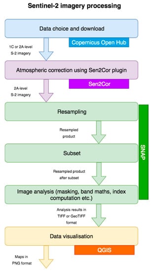
Figure 1.
Sentinel-2 imagery processing flowchart. S-2—Sentinel 2; SNAP—Sentinel Application Platform; TIFF—Tagged Image File Format; QGIS—Quantum GIS.
2.1. Study Area
The study area is located on the Polish side of the Białowieża Forest, which is one of the last and largest remaining parts of the immense primeval forests in Europe. It straddles the border between Poland and Belarus, covering 592 km2 and 753 km2 in those countries, respectively (1345 km2 in total) [13]. The Polish part of the forest is located between 23.52° and 24.35° E longitude and between 52.48° and 52.95° N latitude [14]. The climate in that region is characterized by a cool, temperate continental climate with influence from the Atlantic [13]. For the purpose of the study, atmospheric conditions during relevant time periods were analyzed. Average temperature was higher by 1 °C in the vegetation period of 2016 than in 2018. At the same time, the precipitation sum was greater by 40 and 80 mm during the spring and summer of 2016, respectively. Sun exposure was longer in spring of 2016 by 220 h and in summer of 2018 by 125 h. Additionally, weather conditions in September of both years were compared: precipitation was nearly twice higher in 2018, with comparable sun exposure during both years [15].
The forest is considered one of the best-preserved areas in Poland and has the status of a World Heritage Site. Tree cover in Białowieża Forest is characterized as dense and relatively difficult to penetrate. Hence, precise tree inventory is not easy to carry out. However, a recent study performed as a part of LIFE + ForBioSensing PL project resulted in high accuracy (69–80%) forest classification. It presented forest composition as consisting mainly of spruce, pine, and alder trees (comparable amounts, ca. 20% each), with the addition of lime, hornbeam, birch, and oak trees (between 5 and 11% each), as well as other broadleaves (below 10%) [16]. The forest grows on brown (36%), podzolic (19%), and gley-podzol (12%) soils. The rest of the terrain is covered with black earths, mud, and muck soils [17].
2.2. Data Download and Pre-Processing
Imagery acquired by Sentinel satellites is available for users via the Copernicus Open Access Hub [18]. For the purpose of this work, two images covering the area of interest (Białowieża Forest) were downloaded. They were acquired one year before (17 October 2016) and one year after (12 October 2018) tree logging in 2017. Minimal possible cloudiness level, as well as full tile coverage, was taken into consideration. The following files were downloaded:
- S2A_MSIL2A_20161017T094032_N0204_R036_T34UFD_20161017T094431.SAFE,
- S2B_MSIL2A_20181012T094029_N0209_R036_T34UFD_20181012T145646.SAFE.
Pre-processing of the imagery involved the following steps: atmospheric correction, resampling, and subset.
Atmospheric correction was carried out in the Sen2Core processor provided by the ESA. The process allowed us to remove the influence of the atmosphere on data, while maintaining the original spatial resolution, as well as order of spectral bands of the input imagery. During correction, input level-1C (top-of-atmosphere reflectance) images were converted into level-2A (bottom-of-atmosphere reflectance) products [19]. This way, true surface reflectance could be accessed [20].
After successful atmospheric correction in the Sen2Cor plugin, resulting 2A-level data were imported into SNAP software for further processing. Resampling, the first necessary operation, aimed to geometrically correct distorted pixels in the original imagery. Available resampling methods included: the nearest neighbor, bilinear interpolation, and cubic convolution. The first option was chosen, as it allowed us to preserve the original pixel values. The operation was performed with respect to the B4 band (red) and corresponding 10 m spatial resolution.
Lastly, both images were subsetted to the coordinates of 53.05° N, 23.25° W, 52.30° S, 24.077° E. Hereby, the area of interest was limited to forest boundaries for convenience of analysis.
Performance of the aforementioned procedures resulted in two atmospherically corrected, resampled, subsetted images of 10–60 m spatial resolution (depending on the spectral band).
2.3. Environmental Analysis Tools
As the main part of environmental analysis, a set of radiometric and biophysical indices was computed. The choice of particular indices was based on their availability in SNAP software, as well as on their usefulness for similar studies [21]. Numerous sources describe Normalized Difference Vegetation Index (NDVI) as the most commonly used for vegetation monitoring [22,23,24,25]. A study carried out in the area of Bialowieża Forest showed low NDVI’s sensitivity to varied forest composition [26]. Other indices mentioned in the literature include inter alia, the Ratio Vegetation Index (RVI) [25], the Soil-Adjusted Vegetation Index (SAVI) [27], and the Global Environmental Monitoring Index (GEMI) [28]. The MERIS Terrestrial Chlorophyll Index (MTCI) was also found to accurately depict leaf chlorophyll concentration [29]. The decision to incorporate biophysical processor computations into the study was based on their characteristics described in ESA’s “S2ToolBox Level 2 products” manual [30]. Other indices available in SNAP software were added supplementarily.
Index values were calculated using formulas defined in SNAP, with input reflectance of at least two spectral bands. All equations used in computations were derived from SNAP algorithm specifications [31]. In all cases: Green—B3 band, Red—B4 band, Rededge—B5 band, NIR—B8 band, unless mentioned otherwise.
Radiometric vegetation indices:
- 1.
- Ratio Vegetation Index (RVI)
- 2.
- Difference Vegetation Index (DVI)
- 3.
- Normalized Difference Vegetation Index (NDVI)
- 4.
- Perpendicular Vegetation Index (PVI)
- 5.
- Soil-Adjusted Vegetation Index (SAVI)
- 6.
- Global Environmental Monitoring Index (GEMI)
- 7.
- MERIS Terrestrial Chlorophyll Index (MTCI)
- 8.
- Modified Chlorophyll Absorption Ratio Index (MCARI)
Radiometric soil indices:
- 9.
- Brightness Index (BI)
- 10.
- Color Index (CI)
Biophysical indices:
- 11.
- Leaf Area Index (LAI),
- 12.
- Fraction of Absorbed Photosynthetically Active Radiation (FAPAR),
- 13.
- Fractional Vegetation Cover (FVC or FCOVER),
- 14.
- Chlorophyll content (a + b) (Cab),
- 15.
- Canopy water content (CWC or CW).
For calculation of biophysical indices, input data include spectral information (8 bands: B3–B7, B8a and B11–B12), as well as directional information (cosine of sun zenith angle (θs), view zenith angle (θv), and relative azimuth angle (φ)). Ranges of biophysical indices, according to ESA, are as follows:
0 ≤ LAI ≤ 8 (-),
0 ≤ FAPAR ≤ 1 (-),
0 ≤ FVC ≤ 1 (-),
0 ≤ Cab ≤ 600 (g/cm2),
0 ≤ CWC ≤ 0.55 (μg/cm2) [30].
The subsequent analysis step was band maths computation. The band maths tool available in SNAP enables mathematical calculations between spectral bands of products. To facilitate visual analysis of vegetation cover changes, the difference between 2018 and 2016 index results was computed for each index.
Then, operations allowing for derivation of specific pixel values were carried out, including pin placing and masking. The former enabled us to extract values obtained at single pixels, whereas the latter focused on pixel groups, allowing us to access information regarding whole areas (including simple statistical data). For the purpose of this project, two pins were created: one where tree felling occurred, and one where dense forest remained uninterrupted. Region of interest (ROI) mask consisting of over 4 million pixels were also generated, covering regions of Białowieża Forest with the highest recorded tree logging rate. Study locations were chosen based on the map created by Greenpeace, the organization trying to track logging areas as precisely as possible during the studied period, also in the field [12]. It is necessary to stress that verification of ground-based data was difficult due to the ongoing dispute and events, resulting in poor data availability [32]. For that reason, only one felling site was intentionally chosen for the purpose of this study, as there was full certainty regarding logging occurrence there. Otherwise, identification of other locations could be uncertain.
Pinpoints and ROI mask (visible in Figure 2 and Figure 3) were exported to all other products created during computations. Statistical data regarding regions covered by mask were accessed. These operations allowed for comparison of obtained index values, which will be discussed in detail in the next section.
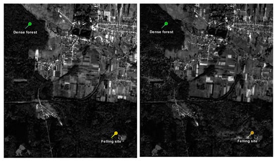
Figure 2.
Pinpoints created for October 2016 (left) and 2018 (right).
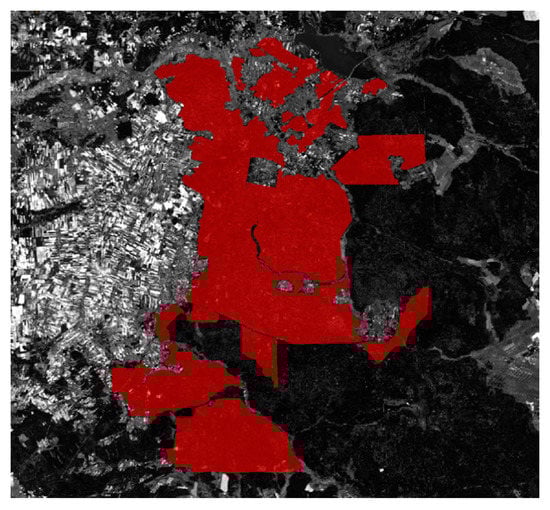
Figure 3.
Region of interest (ROI) mask created over the forest area.
3. Results and Discussion
Pinpoint results enabled us to assess approximate order of magnitude of index values at felled and uninterrupted locations. This information highly facilitated the preparation of color legends in SNAP, necessary for visualization of index values in the form of maps, which are discussed further on in this chapter. Pinpoint index values are presented in Table 2. Mean, median, and standard deviation calculated for ROI mask index values are contained in Table 3.
Table 2.
Index values at pinpoints for years 2016 and 2018. RVI—Ratio Vegetation Index; DVI—Difference Vegetation Index; NDVI—Normalized Difference Vegetation Index; PVI—Perpendicular Vegetation Index; SAVI—Soil-Adjusted Vegetation Index; GEMI—Global Environmental Monitoring Index; MTCI—MERIS Terrestrial Chlorophyll Index; MCARI—Modified Chlorophyll Absorption Ratio Index; BI—Brightness Index; CI—Colour Index; LAI—Leaf Area Index; FAPAR—Fraction of Absorbed Photosynthetically Active Radiation; FCOVER—Fractional Vegetation Cover; Cab—Chlorophyll content (a + b); CW—Canopy water content.
Table 3.
Mean, median, and standard deviation of index values obtained for region of interest (ROI) mask for years 2016 and 2018. RVI—Ratio Vegetation Index; DVI—Difference Vegetation Index; NDVI—Normalized Difference Vegetation Index; PVI—Perpendicular Vegetation Index; SAVI—Soil-Adjusted Vegetation Index; GEMI—Global Environmental Monitoring Index; MTCI—MERIS Terrestrial Chlorophyll Index; MCARI—Modified Chlorophyll Absorption Ratio Index; BI—Brightness Index; CI—Colour Index; LAI—Leaf Area Index; FAPAR—Fraction of Absorbed Photosynthetically Active Radiation; FCOVER—Fractional Vegetation Cover; Cab—Chlorophyll content (a + b); CW—Canopy water content. Bold text distinguishes particular indices.
RVI pinpoint values decreased for both dense forest (DF) and felling site (FS), showing possibly tendentious behavior. However, the decrease at the latter pinpoint was substantially greater (by 43%) than at the former (by 12%). The mean ROI mask value was nearly the same as the DF result in that year, indicating dense forest cover over the whole area of interest. In 2018, the mean value decreased by almost 3 units, corresponding with pinpoint results. Hence, RVI may be displaying potential for forest cover change detection.
DVI increased for both DF and FS. The increase at FS was significantly higher, indicating denser canopy cover after tree felling. Such results were opposite to the expected ones and not compatible with the tree logging map. This tendency was also present for ROI mask mean and median values.
NDVI decreased at both locations. However, the decrease at FS was significantly greater (by 34%) than at DF (by 2%), indicating canopy cover loss over the felling site. According to NDVI value classification [33], medium density canopy cover was present at FS in 2016 and transformed into shrub or grassland area in 2018. At the same time, value characteristics for dense canopy cover were maintained at DF, indicating a lack of major land cover changes. In terms of ROI mask, the mean and median both decreased, indicating a decrease in canopy cover. Hence, NDVI’s potential for deforestation observation could be assessed as high.
PVI, SAVI, and GEMI values rose for both pinpoints, indicating denser canopy cover at FS in 2018, contrary to the expected outcome. Moreover, ROI mask mean and median values behaved similarly to DF pinpoint values. Hence, those indices were not considered of high potential in terms of discussed deforestation observation.
MTCI pinpoint values increased at DF (by 5%), whereas they declined significantly at FS (by 26%). Index behavior indicated the presence of denser forest cover at the former site, with simultaneous canopy cover reduction at the latter. Hence, differently to most vegetation indices, MTCI’s behavior was not tendentious, potentially showing index sensitivity to the changing state of the canopy cover. In terms of the ROI mask mean and median, both values decreased, informing about average canopy cover loss.
MCARI values increased for DF, whereas they remained nearly the same at FS. Hence, no changes after tree logging could be observed. ROI mask results also increased slightly, indicating denser canopy cover in 2016 than in 2018.
In the case of BI, four decimal places were taken into consideration, due to the magnitude of obtained values. BI pinpoint results rose for both DF and FS; however, the increase was significantly greater at the latter site (by 311%) compared to the former (by 31%). Hence, it can be concluded that uncovered soil was detected over FS, which is in correspondence with the expected results. Mean and median obtained for the region of interest also increased, confirming tendency observed at pinpoints.
CI pinpoint results obtained at DF were negative for both terms, depicting lack of visible uncovered soil. At the same time, FS results increased significantly (by 154%), informing about potential bare soil visibility. Mean and median ROI mask results also increased in 2018.
In terms of biophysical indices, the majority of results were higher in 2018 than in 2016 for both pinpoints, with the exception of FAPAR and Cab values obtained at FS. They were higher in the former and lower in the latter term (by 5 and 34%, respectively), displaying non-tendentious behavior. However, due to their magnitude, only Cab’s FS results could be considered significant for the discussed change detection purposes. In terms of ROI mask, mean and median values increased for all biophysical indicators.
To visualize index computation results regarding the whole forest area, color maps were prepared using SNAP and QGIS software. Legends were developed based on indices’ ranges and histograms, as well as on pinpoint values. Moreover, each map had corresponding statistical data computed for ROI mask. In this paper, visualization of RVI results in form of color maps, along with statistical data and histograms computed for ROI mask, are presented in Figure 4, Figure 5, Figure 6, Figure 7, Figure 8 and Figure 9. This particular index has been chosen due to clear visibility of differences between years 2016 and 2018. Maps presenting values of all indices were discussed in the previous paper [34]. Spatial resolution of created outputs corresponded with the resolution of specific spectral bands used in calculations.
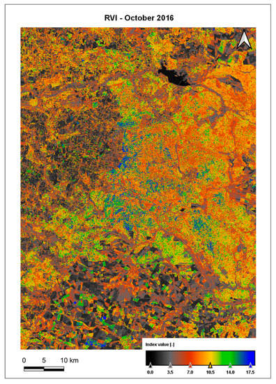
Figure 4.
Map presenting Ratio Vegetation Index (RVI) values obtained for October 2016.

Figure 5.
Statistical data computed for RVI values obtained for October 2016.
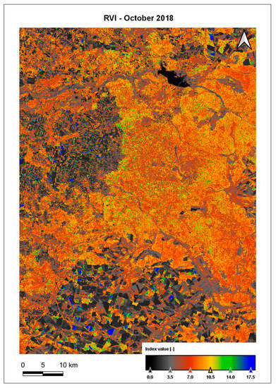
Figure 6.
Map presenting RVI values obtained for October 2018.
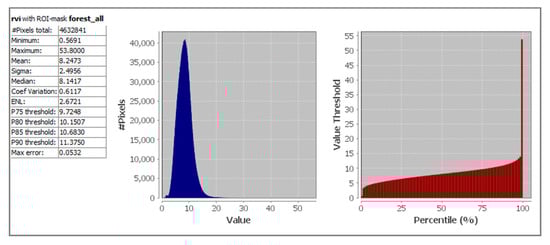
Figure 7.
Statistical data computed for RVI values obtained for October 2018.
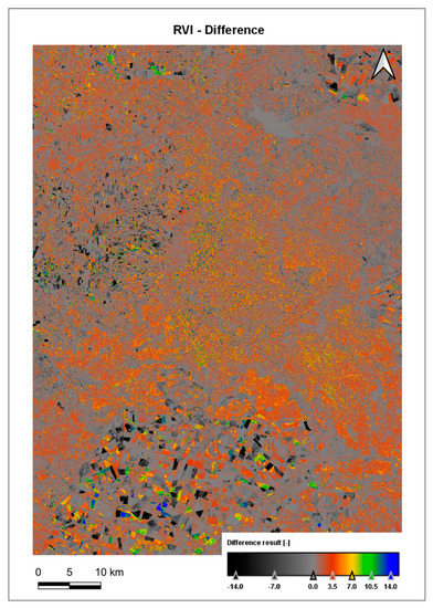
Figure 8.
Map presenting RVI difference results.
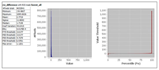
Figure 9.
Statistical data computed for RVI difference results.
4. Conclusions
Successful processing of Sentinel-2 imagery in the Sen2Cor plugin and SNAP software, as well as visualization of final products in the QGIS program, showed it was possible to conduct environmental analysis with the use of only free and available software. SNAP software and the Sen2Cor plugin, along with the Copernicus Open Access Hub database, constituted a professional tool for environmental observation. Computation of radiometric and biophysical indices, performed as a part of this project, allowed us to preliminarily assess the usefulness of particular spectral calculations for deforestation observation.
The majority of vegetation indices did not display the expected behavior. Their values either increased over the felling site (DVI, PVI, SAVI, GEMI) in the latter term, indicating denser canopy cover, or remained similar (MCARI), showing no change. Out of eight chosen radiometric vegetation indices, three were successful in the depiction of forest cover change: RVI, NDVI, and MTCI. They showed significant canopy cover decrease over the felling area. Additionally, MTCI’s behavior was not tendentious, as its value increased for the dense forest pinpoint. This fact could indicate high sensitivity to canopy cover changes and, hence, high potential for deforestation observation.
Soil indices appeared to be successful in differentiation between felled and uninterrupted forest areas. The Brightness Index (BI) displayed the greatest difference between values obtained at the felling site in 2016 and 2018, considering the whole set of indices. Such clear distinction between land cover types may have resulted from the fact that soil was environmentally more stable than the vegetation, with the latter being largely influenced by changing climate conditions.
In terms of biophysical indicators, only Chlorophyll a + b (Cab) provided results relevant for deforestation observation. The rest of indices did not provide expected results.
Eleven out of fifteen indices indicated an increase in vegetation cover over the dense forest site. This could have resulted from the considerably higher precipitation sum in September of 2018, the month prior to data acquisition. This situation could have also influenced the results over the tree felling site. However, according with the expected results, tree logging should be a precedent cause for index behavior.
Additionally, very good agreement was found between the values of all fifteen indices determined at the chosen pin locations and the mean values of those indices calculated from all pixels (over 4 million) on the masked area, before (2016) and after logging (2018). It was clearly visible when comparing respective values of indices.
Advanced satellite imagery processing tools provided by the ESA enabled complex forest cover analysis, successfully carried out and presented in this study. It is necessary to mention that the methodology described in this work may be of use when detailed information regarding tree logging is not available. The results of this project are promising, showing high potential for ex-situ forest cover change observations. They can also constitute a strong base for further investigations.
Author Contributions
Conceptualization, K.W.P. and J.Z.; methodology, K.W.P. and J.Z.; software, K.W.P.; validation, K.W.P. and J.Z.; formal analysis, K.W.P. and J.Z.; investigation, K.W.P. and J.Z.; resources, K.W.P.; data curation, K.W.P.; writing—original draft preparation, K.W.P.; writing—review and editing, K.W.P. and J.Z.; visualization, K.W.P.; supervision, J.Z.; funding acquisition, J.Z. All authors have read and agreed to the published version of the manuscript.
Funding
The research leading to these results received funding from the statutory activities of Faculty of Building Services, Hydro and Environmental Engineering of Warsaw University of Technology.
Conflicts of Interest
The authors declare no conflict of interest.
References
- ESA. Sentinel Online. Sentinel-2. Available online: https://sentinel.esa.int/web/sentinel/missions/sentinel-2 (accessed on 18 June 2020).
- ESA. Science Toolbox Exploitation Platform (STEP). Sentinel Application Platform (SNAP). Available online: https://step.esa.int/main/toolboxes/snap (accessed on 25 June 2020).
- Milodowski, D.; Mitchard, E.; Williams, M. Forest loss maps from regional satellite monitoring systematically underestimate deforestation in two rapidly changing parts of the Amazon. Environ. Res. Lett. 2017, 12, 094003. [Google Scholar] [CrossRef]
- USAID. Overview of semi-automated approaches for monitoring national deforestation. In Forest Carbon, Markets and Communities (FCMC) Program; USAID: Washington, DC, USA, 2015. [Google Scholar]
- EU SCIENCE HUB. European Commission’s Science and Knowledge Service. A Comparison of US and EU Satellites in Monitoring Forest Disturbances. 2019. Available online: https://ec.europa.eu/jrc/en/science-update/comparison-us-and-eu-satellites-monitoring-forest-disturbances (accessed on 18 June 2020).
- Simonetti, D.; Marelli, A.; Rodriguez, D.; Vasilev, V.; Strobl, P.; Burger, A.; Soille, P.; Achard, F.; Eva, H.; Stibig, H.J.; et al. Sentinel-2 web platform for REDD+ monitoring. In JRC Technical Reports; European Commission: Brussels, Belgium, 2017. [Google Scholar]
- Addabbo, P.; Focareta, M.; Marcuccio, S.; Votto, C.; Ullo, S.L. Contribution of Sentinel-2 data for applications in vegetation monitoring. In ACTA IMEKO; IMEKO: Budapest, Hungary, 2016; Volume 5, pp. 44–54. ISSN 2221-870X. [Google Scholar]
- Hawryło, P.; Wężyk, P. Predicting Growing Stock Volume of Scots Pine Stands Using Sentinel-2 Satellite Imagery and Airborne Image-Derived Point Clouds. Forests 2018, 9, 274. [Google Scholar] [CrossRef]
- Spectral Reflectance. Humboldt State Geospatial Online. Humboldt State University. Available online: http://gsp.humboldt.edu/OLM/Courses/GSP_216_Online/lesson2-1/reflectance.html (accessed on 17 June 2020).
- Mikusiński, G.; Bubnicki, J.W.; Churski, M.; Czeszczewik, D.; Walankiewicz, W.; Kuijper, D.P. Is the impact of loggings in the last primeval lowland forest in Europe underestimated? The conservation issues of Białowieża Forest. Biolog. Conserv. 2018, 227, 266–274. [Google Scholar] [CrossRef]
- Commission Calls for Immediate Suspension of Logging in Poland’s Białowieża Forest. European Commision, European Union. 13 July 2017. Available online: https://ec.europa.eu/commission/presscorner/detail/pl/IP_17_1948 (accessed on 1 August 2020).
- Bohdan, A.; Grundland, M.R.; Kolbusz, M.; Książek, M.; Mikos, A.; Rok, J. Report on the Devastation of the Forest, 2017; Greenpeace: Warszawa, Poland, 2018; Available online: https://www.greenpeace.org/poland/raporty/1119/raportz-dewastacji-puszczy-2017 (accessed on 15 June 2020).
- Więcko, E. Białowieza Primeval Forest; Wydawnictwo Naukowe (PWN): Warszawa, Poland, 1984. [Google Scholar]
- Karczewska, M. Location. Białowieża National Park. Available online: https://bpn.com.pl (accessed on 18 June 2020).
- Climate Maps of Poland. CLIMATE IMGW-PIB. Available online: https://klimat.imgw.pl/pl/climate-maps (accessed on 19 June 2020).
- Modzelewska, A.; Fassnacht, F.E.; Stereńczak, K. Tree species identification within an extensive forest area with diverse management regimes using airborne hyperspectral data. Int. J. Appl. Earth Obs. Geoinf. 2020, 84, 101960. [Google Scholar] [CrossRef]
- Program Ochrony Przyrody i Wartości Kulturowych w Leśnym Kompleksie Promocyjnym Puszcza Białowieska na okres 1.01.2002–31.12.2011; Regionalna Dyrekcja Lasów Państwowych w Białymstoku: Warsaw, Poland, 2011.
- Copernicus Open Access Hub. Copernicus, ESA. 2019. Available online: https://scihub.copernicus.eu/dhus (accessed on 21 June 2020).
- Sen2Cor. STEP ESA. Available online: http://step.esa.int/main/third-party-plugins-2/sen2cor (accessed on 15 June 2020).
- Atmospheric Correction. University of Maryland Institute for Advanced Computer Studies, UMIACS. Available online: http://www.umiacs.umd.edu/research/GC/atmo (accessed on 5 August 2020).
- Da Silva, V.S.; Salami, G.; Da Silva, M.I.; Silva, E.A.; Monteiro Junior, J.J.; Alba, E. Methodological evaluation of vegetation indexes in land use and land cover (LULC) classification. Geol. Ecol. Landsc. 2019, 4, 159–169. [Google Scholar] [CrossRef]
- Change Detection of Vegetation Cover, Using Multi-Temporal Remote Sensing Data and GIS Techniques. Geospatial World. 2009. Available online: https://www.geospatialworld.net/article/change-detection-of-vegetation-cover-using-multi-temporal-remote-sensing-data-and-gis-techniques (accessed on 15 June 2020).
- Othman, M.A.; Ash’Aari, Z.H.; Aris, A.Z.; Ramli, M.F. Tropical deforestation monitoring using NDVI from MODIS satellite: A case study in Pahang, Malaysia. In IOP Conference Series: Earth and Environmental Science; IOP Publishing: Bristol, UK, 2018; Volume 169. [Google Scholar] [CrossRef]
- Vilhar, U.; Beuker, E.; Mizunuma, T.; Skudnik, M.; Lebourgeois, F.; Soudani, K.; Wilkinson, M. Tree Phenology. In Forest Monitoring—Methods for Terrestrial Investigations in Europe with an Overview of North America and Asia; Elsevier: Amsterdam, The Netherlands, 2013; Volume 12, pp. 169–182. [Google Scholar] [CrossRef]
- Myneni, R.B.; Hall, F.G.; Sellers, P.J.; Marshak, A.L. The Interpretation of Spectral Vegetation Indexes. In IEEE Transactions on Geoscience and Remote Sensing; IEEE: New York, NY, USA, 1995; Volume 33, pp. 481–486. [Google Scholar] [CrossRef]
- Bochenek, Z.; Ziolkowski, D.; Bartold, M.; Orlowska, K.; Ochtyra, A. Monitoring forest biodiversity and the impact of climate on forest environment using high-resolution satellite images. Eur. J. Remote Sens. 2017, 51, 166–181. [Google Scholar] [CrossRef]
- Bader, A.; El Battay, A.; Belaid, M.; Nadi, M. Comparative Study of SAVI and NDVI Vegetation Indices in Sulaibiya Area (Kuwait) Using Worldview Satellite Imagery. Int. J. Geosci. Geomat. 2013, 1, 50–53. [Google Scholar]
- Schultz, M.; Clevers, J.G.; Carter, S.; Verbesselt, J.; Avitabile, V.; Quang, H.V.; Herold, M. Performance of vegetation indices from Landsat time series in deforestation monitoring. Int. J. Appl. Earth Obs. Geoinf. 2016, 52, 318–327. [Google Scholar] [CrossRef]
- Frampton, W.J.; Dash, J.; Watmough, G.; Milton, E.J. Evaluating the capabilities of Sentinel-2 for quantitative estimation of biophysical variables in vegetation. ISPRS J. Photogram. Remote Sens. 2013, 82, 83–92. [Google Scholar] [CrossRef]
- Weiss, M.; Baret, F. S2ToolBox Level 2 Products: LAI, FAPAR, FCOVER. Version 1.1. STEP, ESA. 2 May 2016. Available online: http://step.esa.int/docs/extra/ATBD_S2ToolBox_L2B_V1.1.pdf (accessed on 15 June 2020).
- Sentinel Application Platform (SNAP). STEP, ESA, 6.0.0. Available online: https://step.esa.int/main/toolboxes/sentinel-2-toolbox/sentinel-2-toolbox-features/ (accessed on 15 June 2020).
- Konarzewski, M.; Zabielski, R.; Kowalczyk, R.; Duszyński, J. Białowieża Forest: Logging data lacking. Science 2018, 359, 646. [Google Scholar] [CrossRef] [PubMed]
- Normalized Difference Vegetation Index. Custom-Scripts. Sentinel-Hub. Available online: https://custom-scripts.sentinel-hub.com/custom-scripts/sentinel-2/ndvi (accessed on 18 June 2020).
- Pałaś, K.W. Sentinel-2 Imagery Processing in Snap Software for Environmental Analysis on the Example of Bialowieza Forest. Bachelor’s Thesis, Warsaw University of Technology, Warszawa, Poland, September 2019. [Google Scholar]
© 2020 by the authors. Licensee MDPI, Basel, Switzerland. This article is an open access article distributed under the terms and conditions of the Creative Commons Attribution (CC BY) license (http://creativecommons.org/licenses/by/4.0/).