Article

Allometric Equations for Predicting Agave lechuguilla Torr. Aboveground Biomass in Mexico

by
Cristóbal de J. Flores-Hernández
1,
Jorge Méndez-González
1,*,
Félix de J. Sánchez-Pérez
2,
Fátima M. Méndez-Encina
1,
Óscar M. López-Díaz
1 and
Pablito M. López-Serrano
3
1
Forest Department, Autonomous Agrarian University Antonio Narro, Coahuila P. C. 25315, Mexico
2
Independent Statistical Consultant, Coahuila P. C. 25315, Mexico
3
Institute of Forestry and Wood Industry, Juarez University of the State of Durango, Durango P. C. 34120, Mexico
*
Author to whom correspondence should be addressed.
Forests 2020, 11(7), 784; https://doi.org/10.3390/f11070784
Submission received: 15 June 2020 / Revised: 9 July 2020 / Accepted: 10 July 2020 / Published: 21 July 2020
(This article belongs to the Special Issue Assessing, Valuing and Mapping Ecosystem Services)

Abstract

:
Quantifying biomass is important for determining the carbon stores in land ecosystems. The objective of this study was to predict aboveground biomass (AGB) of Agave lechuguilla Torr., in the states of Coahuila (Coah), San Luis Potosí (SLP) and Zacatecas (Zac), Mexico. To quantify AGB, we applied the direct method, selecting and harvesting representative plants from 32 sampling sites. To predict AGB, the potential and the Schumacher–Hall equations were tested using the ordinary least squares method using the average crown diameter (Cd) and total plant height (Ht) as predictors. Selection of the best model was based on coefficient of determination (R2 adj.), standard error (Sxy), and the Akaike information criterion (AIC). Studentized residues, atypical observations, influential data, normality, variance homogeneity, and independence of errors were also analyzed. To validate the models, the statistic prediction error sum of squares (PRESS) was used. Moreover, dummy variables were included to define the existence of a global model. A total of 533 A. lechuguilla plants were sampled. The highest AGB was 8.17 kg; the plant heights varied from 3.50 cm to 118.00 cm. The Schumacher–Hall equation had the best statistics (R2 adj. = 0.77, Sxy = 0.418, PRESS = 102.25, AIC = 632.2), but the dummy variables revealed different populations of this species, that is, an equation for each state. Satisfying the regression model assumptions assures that the predictions of A. lechuguilla AGB are robust and efficient, and thus able to quantify carbon reserves of the arid and semiarid regions of Mexico.

1. Introduction

Climate change is a problem of great magnitude. From 1950 to 2014, CO2 emissions increased from 310 to 400 ppm [1], and currently the concentration is 409.92 ppm [2]. Forest ecosystems play an important role in regulating the climate by absorbing carbon [3] into plant biomass through photosynthesis [4]. Like many countries, Mexico has developed public policies to improve the well-being of the communities that live in arid regions. It has also developed a National Strategy for Reducing Emissions due to Deforestation and forest Degradation (ENAREDD+, the initials in Spanish), which aims decelerate, stop, and reverse loss of forest cover and increase carbon sequestering and ecosystem services through sustainable management [5], to contribute to climate change mitigation. Arid regions are the most vulnerable to climate change [6]. Conservation and improvement of these areas is an option for maintaining carbon reserves [7]. Of Mexico’s territory, 54% is arid, and more than 40% of the population live in these regions; however, it is known that above (23.2 Mg ha−1 ± 4.15 Mg ha−1) and underground biomass (11.2 Mg ha−1 ± 3.54 Mg ha−1) is more than the average (2 Mg ha−1 to 5 Mg ha−1) that exists in the world’s deserts [8].
The UN Framework on Climate Change considers plant biomass as a necessary variable for prediction and mitigation of climate change [9]. Quantifying plant biomass allows us to determine how much carbon is stored in ecosystems [10]. For this reason, aboveground biomass equations are fundamental to evaluating carbon stores [11]. Aboveground biomass of some scrub vegetation and grasslands in arid and semiarid regions of Mexico varies from 1.6 to 30 Mg ha−1, while stored carbon varies from 1 to 15.5 Mg C ha−1 [12]. Agave lechuguilla Torr., locally called “lechuguilla”, is distributed in arid and semiarid regions of the Chihuahua desert in Mexico and southern USA [13]. From this plant a fiber known as “ixtle” is extracted; ixtle is used to make brushes, mats, bags, and many other industrial products [14].
Aboveground biomass in plant species has been estimated by: (a) direct methods, in which complete plants are harvested to obtain fresh and dry weight [15]; and (b) by indirect methods, allometric equations developed from the first method [11,16]. Recently, the two procedures have been combined: aboveground biomass is estimated with remote sensors, the estimation is validated in the field with direct measurements and, using different algorithms [17], such as ordinary least squares, random forest or support vector regression [18,19,20], and the equations are generated. This type of equation uses dasometric variables that are easily measured, such as tree diameter, total height, and crown diameter, and are correlated with biomass [15]. Its predictive capacity depends on whether the assumptions of regression, such as normality, homogeneity of variance, and independence, are satisfied [21,22,23]. In this type of model it is possible to include indicator or dummy variables, which are variables that take values of 0, 1, or −1 to indicate absence or presence of some categoric effect [24] and that are useful to differentiate a set of data that belong to independent samples and, in this way, identify one or more models [25,26]. This method has been shown to be effective for resolving compatibility of biomass estimations at different scales [27].
Evidence reveals a scarcity of models of aboveground biomass (AGB) for arid regions’ species, except for the study by Pando-Moreno et al. [28] which estimated usable fiber. Others have calculated the time of harvesting [29] or characterized the ecosystems where the plant grows [30,31]. The objective of our study was to fit two allometric equations using dummy variables for predicting aboveground biomass of A. lechuguilla samples from the Mexican states of Coahuila, Zacatecas, and San Luis Potosí.

2. Materials and Methods
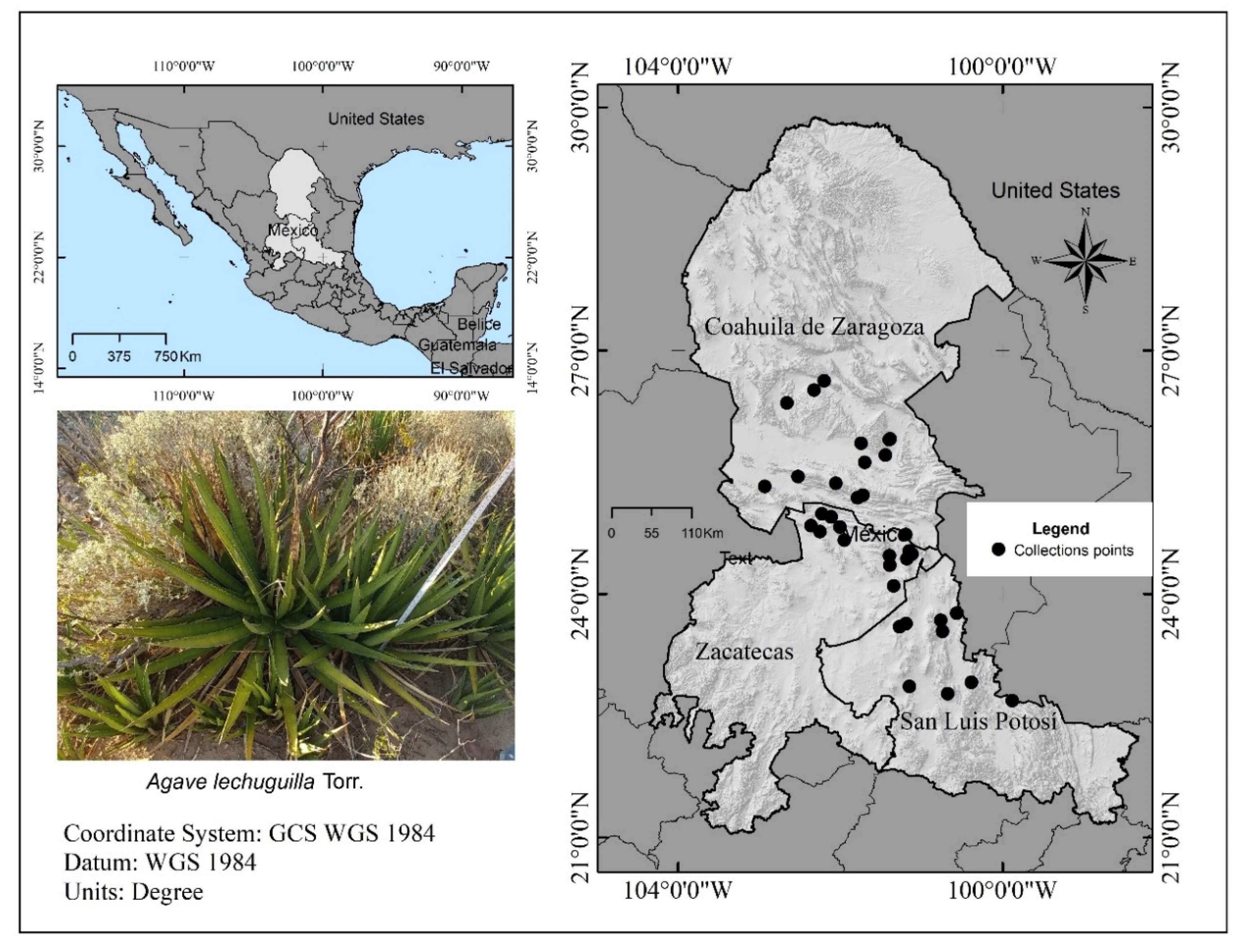
2.1. Study Area

The study was conducted in north-central Mexico (99°48′–103° W, 22°50′–26°38′ N) in three states (Figure 1): Coahuila (Coah); San Luís Potosí (SLP); and Zacatecas (Zac). The predominant vegetation is rosetophile scrub and, in a lesser proportion, microphile scrub [32,33], made up mostly of Agave lechuguilla and genera such as Dasylirion sp., Larrea sp., Opuntia sp., Acacia sp., and species of the family Cactaceae [30,33]. Altitude varies from 810–2166 m; climate type is very arid and warm (BWhw) and arid temperate (BSokw). Mean annual precipitation varies from 126–600 mm and mean annual temperature is 16–22 °C [34].

2.2. Sampling of Aboveground Biomass

Based on Picard et al. [15], the direct method was applied to quantify the AGB of A. lechuguilla. Sampling was conducted only in “ejidos” and communities with permission to exploit plants of this species. For sample collection, the central part of the managed area was located and a radius of approximately 1 km was drawn; n number of plants were selected considering all the existing sizes (diameter, height and crow diameter). Each plant was measured for crown diameter (Cd) and total height (H) with a 3 m tape measure (Truper®). The selected plants were then cut (only the aerial part) with manual tools to obtain fresh weight immediately on a 5 kg capacity Torrey® (model L-EQ) scale with a precision of 1 g. A subsample of all these aerial components was taken from each plant, with which its fresh weight was determined. The subsamples were taken to the laboratory and dried in an electric oven (mark Thermo Scientific™ HERAtherm™, model OMH750) at 70 °C until a constant weight was obtained. With this data, the ratio between dry and fresh weight was determined and multiplied by the total fresh weight per plant to obtain total dry biomass or AGB [11,15].

2.3. Statistical Analysis

To determine A. lechuguilla AGB, the potential (Equation (1)) and the Schumacher–Hall [35] (Equation (2)) equations were used, both in their linearized form. These equations have been demonstrated to fit well and give reliable predictions of AGB of different forest species [4,11,36,37].
ln ( A G B P o t e n t i a l ) = ln β 0 + ln β 1 × ln ( C d ) + ε
ln ( A G B S c h u m a c h e r H a l l ) = ln β 0 + β 1 × ln ( C d ) + β 2 × ln ( H ) + ε
where AGB is dry aboveground biomass (kg), Cd is the average crown diameter (cm), H plant height (cm), ln natural logarithm, βij are regression coefficients, and ε the random error of the model.
To determine the existence of one or more models, dummy variables were added thus denoting the states, and leaving k−1 dummy variable based on the proposal of Montgomery et al. [22] and Fox [25]. An affectation to the intercept was considered (without interaction of the quantitative dummy variable), and the slope of the model (quantitative dummy interaction), resulting in Equations (3) and (4).
ln ( A G B P o t e n t i a l ) = ln β 0 + β 1 ln ( C d ) + β 2   ( Z a c ) + β 3   ( S L P ) + β 4   ( Z a c : C d ) + β 5   ( S L P : C d ) + ε
ln ( A G B S c h u m a c h e r H a l l ) = ln β 0 + β 1   l n ( C d ) + β 2   l n ( H ) + β 3   ( Z a c ) + β 4   ( S L P ) + β 5   ( Z a c : C d ) + β 6   ( Z a c : H ) + β 7   ( S L P : C d ) + β 8   ( S L P : H ) + ε
Statistical analyses were performed in R [38]. The models were fit using the ordinary least squares (OLS) method [22] using the ‘stats’ library and applying the correction factor by logarithmic transformation [39]. This method is widely used because the statistical–mathematical solution to obtain the regression coefficients is simple, minimizing the sum of squares of the observations with a linear relationship. Furthermore, this method allows the basic assumptions of a regression model to be met [25,26]; likewise, the use of logarithms by linearization of the model reduces the variance of the error and corrects model inadequacies [22,40]. Selection of the best model was based on the best coefficient of determination (R2 adj.), the smallest standard error (Sxy), and value of the Akaike information criterion (AIC). To validate the models, the statistic prediction error sum of squares (PRESS), calculated with the ‘qpcR’ library [41], was used. This statistic is considered a form of crossed validation, as well as a way to evaluate the predictive capacity of a regression model [42].

2.4. Adaptation of the Regression Model

Atypical data in a regression model cause the noncompliance of the regression assumptions [25,43] and, thus, bias in the predictions. Based on the studentized residues of the model, atypical observations were identified, and values equal to or greater than 3 were eliminated from the analysis. Simultaneously, influencing data were evaluated with the ‘stats’ library [44]. With the ‘nortest’ library [45], normality of residuals was diagnosed using the Lilliefors test; variance homogeneity was verified using the Breusch-Pagan test of the ‘lmtest’ library [46], and independence of errors was checked with the Ljung-Box test [44]. When considering the multiple model, collinearity diagnostic was performed using the variance inflation factor (VIF) of the ‘stats’ library and the condition number or index (CN) based on eigenvalues [22].

2.5. Robust Regression Techniques

When the assumptions of regression are not satisfied by the effects of heavier, or atypical, observations, methods alternate to OLS are employed [21]. These methods consist of reducing the effect of these observations, as robust regression techniques or, in its case, generalized least squares [21,22,47]. Here, we applied the method of high breaking point estimation (MM estimation) proposed by Yohai [48] and derived from the maximum likelihood method (M estimation) proposed by Huber [49], using robust scale estimation (S estimation). The second method, least trimmed squares (LTS), minimizes the sum of squares of the smallest k residues and tolerates a large quantity of atypical values [21], both analyzed with the ‘robustbase’ library [50]. The method of least absolute deviation (LAD) minimizes the sum of absolute residues [51] in the ‘L1pack’ library [52] and generalized least squares (GLS) that estimate the coefficients of regression through iterative processes, based on the maximum likelihood method [53] and analyzed in the ‘nlme’ library [54]. In addition, the mean square error (MSE) and the R2 adj. (adjusted coefficient of determination) were examined, and the regression assumptions of each method were verified.

3. Results and Discussion

3.1. Descriptive Statistics Within Its Algorithm

We sampled 533 A. lechuguilla plants distributed in the following manner: 175 in Coah, 178 in SLP, and 180 in Zac (Supplementary Materials). Plant size varied (Table 1). Plant height varied from 3.50 to 118.00 cm, Pando-Moreno et al. [28] reported heights between 25 and 97 cm for the same species in Coahuila and Tamaulipas. However, the analysis of variance (AOV) and the least significant difference (LSD) test showed that there were no statistically significant differences in Cd (p > 0.05) and H (p > 0.05) among states, but for AGB there were significant differences (p < 0.05); the highest average was found in SLP (0.89 kg plant−1). According to Nobel and Quero [13], biomass is distributed as follows: 60% in leaves, 10% in core, and 4% in roots. The highest AGB registered for the species was 8.17 kg in SLP, followed by Zac with 2.91 kg, and 2.03 kg for Coah. Conti et al. [55] reported that aboveground biomass in eight species that grown in semi-arid conditions oscillates from 0.1 to 25.2 kg.

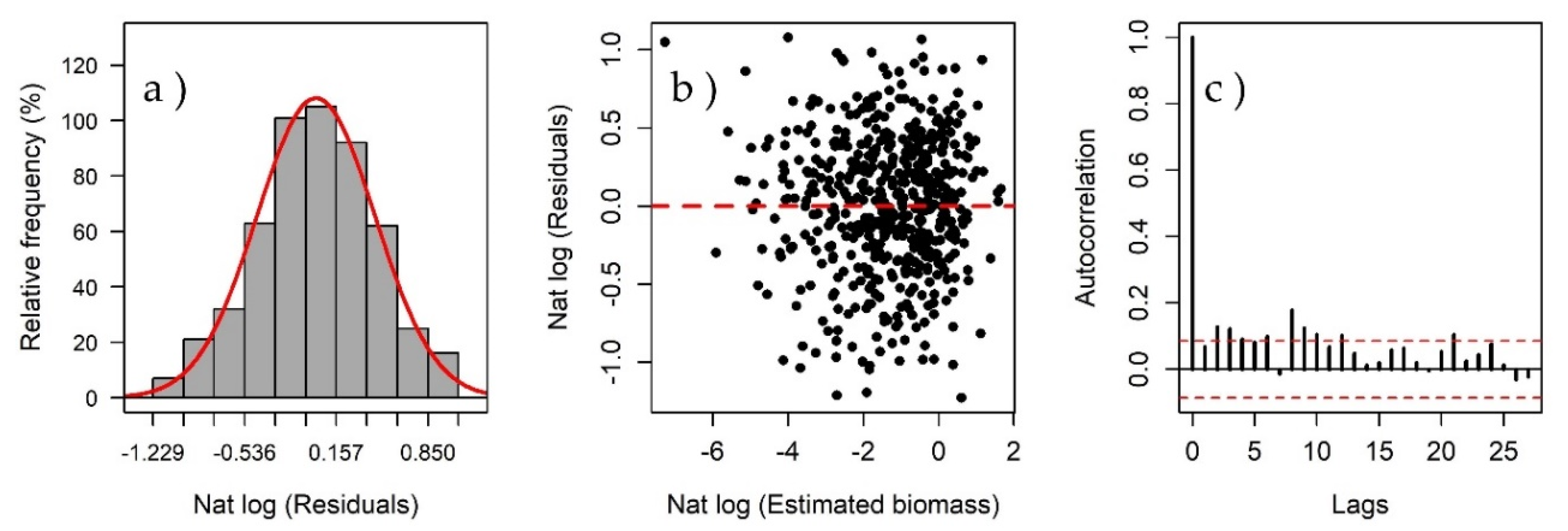
3.2. Model Fit and Detection of Atypical Observations

Estimation of the regression coefficients by OLS showed that, for Equation (3), the coefficient of regression for Cd (β1) and the indicator for Zac (β2) were statistically significant (p < 0.0001) (Table 2), determining an independent model for predicting AGB in Zac (Equation (3a)).
A G B Z a c = ( β 0 + β 2   [ Z a c ] ) + β 1 × ln ( C d )
A G B C o a h   y   S L P = β 0 + β 1 × ln ( C d )
In Equation (4) the coefficients for Cd (β1), H (β2) and the indicators Zac (β3) and SLP (β4) were significant (p < 0.0001) (Table 2), indicating a model for predicting AGB in each state (Equations (4a) to (4c)).
A G B S L P = ( β 0 + β 4   [ S L P ] ) + β 1 ln ( C d ) + β 2 ln ( H )
A G B C o a h = β 0 + β 1 ln ( C d ) + β 2 ln ( H )
A G B Z a c = ( β 0 + β 3   [ Z a c ] ) + β 1 ln ( C d ) + β 2 ln ( H )
where AGB is dry aboveground biomass (kg), Cd is the average crown diameter (cm), H is total height (cm), βij are coefficients of regression, and ln is the natural logarithm.
The use of dummy variables in the AGB equation showed differences among states, affecting the independent term (β0). Aquino et al. [56] applied this type of dummy variable to differentiate groups of species (Cupania dentata DC., Alchornea latifolia Sw. and Inga punctata Willd) when they estimated AGB in southern Oaxaca, Mexico. Also, Cortés et al. [57] estimated AGB in six species of the genus Quercus in Guanajuato, Mexico.
Analysis of studentized residuals detected five atypical data for Equation (3) and nine for Equation (4) (Figure 2a,b); these were eliminated, and the equations were again fit with 527 and 524 data points respectively (Figure 2c,d), resulting in new coefficients of regression (Table 3). Faraway [21] and Fox [25] have demonstrated that this type of observation tends to bias the variance in regression coefficients and, because the model assumptions are not satisfied, the prediction is not robust and affects the direction of the regression slope [43]. For this reason, it is necessary to assure that atypical observations are not the product of mistakes in capturing the information or of errors of measuring tools [58].

3.3. Selection of the Best Model

Equation (4) had the best statistics: significant coefficients of regression (p < 0.0001); smallest standard error (Sxy = 0.439); and the lowest AIC (632), with an acceptable R2 adj. (0.914). Moreover, it had a lower PRESS value (102.25), demonstrating the model’s good predictive capacity [42], where Cd and H explain 91.4% of the variation in A. lechuguilla AGB. The correction factor (by transformation logarithmic) was 1.101 (Table 3). According to Ali et al. [59], the combination of these variables (Cd and H) and the use of the natural logarithm better predicts AGB in shrub species. For the above, this equation was selected to predict aboveground biomass by state (Figure 3). The Schumacher–Hall model showed good fit for estimating leaf biomass in arid region plants in Mexico, e.g., Litsea parvifolia (Hemsl.) and Lippia graveolens Kunth, with R2 of 0.820 and 0.810, respectively [36,60], and total biomass in Euphorbia antisyphilitica Zucc, with R2 of up to 0.897 [37] using Cd, base diameter and H. The β1 coefficients reported in these studies (1.994, 1.935, and 1.611–1.703) were higher than that of A. lechuguilla, and β2 coefficients (0.251, 0.257 y 0.300–0.774) were lower. Logically, these discrepancies are due to different AGB of each species. The usable fiber of A. lechuguilla can be estimated adequately with the polynomial model (R2 = 0.869) using core height and diameter as predictor variables [28].
In tree species, Equation (4) has had good fit (R2 adj. 0.971) for estimating aboveground biomass of Quercus sp. in Guanajuato, Mexico, using diameter at breast height (Dbh) and H as predictors [57], as with tropical species (Cupania dentata DC., Alchornea latifolia Sw. and Inga punctata Willd) with R2 adj. > 0.98 [56]. Araujo et al. [61] used the same equation in 111 trees belonging to 50 tropical species in restoration areas in Rio de Janeiro, Brazil, with an R2 of only 0.65, a β1 lower than that found in our study (0.91), and a higher β2 (1.62), using diameter at breast height (Dbh) and height (H) as predictors.
Equation (3) explained only 87.70% of the AGB of A. lechuguilla and gave higher values of Sxy (0.531) and AIC (834) than Equation (4). Equation (3) has been used to predict AGB in arid region species in Mexico, such as Prosopis sp. [11,62] and in central Asia in Hardwickia binata Roxb. [16] recording an R2 between 0.70 and 0.99. In bushy species (Calligonum polygonoides L.) Singh and Singh [4] obtained an R2 of 0.95; because of the nature of this plant, it was used as a predictor of biomass, the square root of the number of plants stems resulting in β1 = 3.065, higher than that of our study (β1 = 2.014). Ali et al. [59] used this same equation with eight shrub species and trees of less than 5 cm Dbh in a subtropical forest in China to estimate AGB, and obtained varying R2 values (0.59–0.99). Conti et al. [55] developed equations for eight species of a semi-arid forest in Argentina, where they reported an R2 of 0.61–0.85 for the multiple model using the variables crown, total height, number of branches, and diameter of the largest stem. In another study, Zeng et al. [63] used the quadratic model for total biomass prediction in four subtropical shrub species in China, obtaining an R2 above 0.95 with the variables base diameter and height. This reveals the large diversity of allometric models used to quantify AGB, as well as the need to develop specific equations.
Three equations were derived from Equation (4) by effect of the dummy variables. By substituting the values of the coefficient of regression and adding the correction factor, we derived Equations (4d) to (4f) as follows:
A G B S L P = exp [ 10.038 + 1.158 × ln ( C d ) + 1.236 × ln ( H ) ] × 1.101
A G B C o a h = exp [ 10.182 + 1.158 × ln ( C d ) + 1.236 × ln ( H ) ] × 1.101
A G B Z a c = exp [ 10.359 + 1.158 × ln ( C d ) + 1.236 × ln ( H ) ] × 1.101
where AGB is dry aboveground biomass (kg), Cd is average crown diameter (cm), H is total height (cm), and ln is natural logarithm.
The relationship between observed AGB and estimated AGB had a strong linear correspondence (1:1 relation), with intercept (β0) and slope (β1) close to zero and one, respectively (SLP: β0 = −0.09, β1 = 0.92; Coah: β0 = −0.11, β1 = 0.92; Zac: β0= −0.18, β1 = 0.88). This demonstrates the high predictive capacity of the model to estimate AGB of A. lechuguilla [23]. The technique has also been used with E. antisyphilitica [37], Tamarindus indica L. [64], and woody bush species of the Sonora Desert, Mexico [65]. According to Brown [66], one of the concerns in estimating biomass and carbon reserves is the possible error that can occur, from measuring different parameters to error in the final regression model. Cunia [67] attributes these possible errors to the sampling design. However, a review of the literature reveals that few comply with the assumptions of the regression models. In our study, we were very strict in this sense, and the estimations of AGB of Agave lechuguilla were efficient and robust.

3.4. Model Validation

The Lilliefors test in Equation (4) showed normality of residuals (D = 0.020, p value = 0.863) (Figure 4a). According to Fox [25], the coefficients of regression are efficient when this assumption is satisfied. Alonso and Montenegro [68] showed that satisfying normality improves estimations of the dependent variable. The Breusch–Pagan test denoted the residues as homoscedastic (BP = 4.580, df = 4, p = 0.333) (Figure 4b); when this assumption is not satisfied (heteroscedasticity), the coefficients are not efficient for any sample size [69]. The Ljung-Box test revealed that the residues are not correlated (χ2 = 2.371, df = 1, p = 0.124) (Figure 4c). These results suggest that the error variance is adequately estimated; the confidence intervals and the estimations of A. lechuguilla AGB are efficient and unbiased [22].
In some cases, validation of equations is directed toward selection of the best statistics for their predictive capacity and, in the best of cases, to distribution of the residuals (e.g., Owate et al. [70]; Moore [71]; Zeng et al. [63]), leaving aside parametric tests that could verify regression assumptions and corroborate efficiency of the coefficients.
The H matrix, or Hat values, detected five potentially influencing observations, surpassing the critical value given by hii = (3 × k)/n = 0.029, where k is the number of coefficients of regression and n the sample size (Figure 4a). The highest values are found in observations 354 and 357 (hii = 0.05 and 0.06, respectively). Therefore, this type of observation does not exert a leveraging effect on the regression slope [22]. The DFFITS (difference in fits) statistic identified three influencing observations (p < 0.01), surpassing the limit given by 2√(k/n) = 0.195 (Figure 4b). These observations have a slight influence in A. lechuguilla AGB estimation [22,72]. Verification of influencing observations after fitting any equation provides relevant information when considering omission or not of an observation [26]. These observations were not removed from the database. Observation 354 is influential both potentially and in estimation, but it is distributed on the same cartesian plane as the rest of the observations (Figure 5).
Equation (4) did not have serious collinearity; the VIF values of both variables were less than 10 (Cd = 5.64 and H = 5.66). VIF values above 10 in a regressor indicates problems of collinearity [47]; others consider a problem to exist when values are above 5 [22]. The condition number (CN) proposed by Montgomery et al. [22] demonstrated that there is moderate collinearity for H (CN = 193.85) and null collinearity for Cd (CN = 7.90). Therefore, application of a corrective method, such as ridge regression, principal components, or partial least squares, was not necessary [21].

3.5. Robust Estimation

Application of the robust techniques tested in Equation (4) to determine whether to conserve atypical data or not was highly significant (p < 0.0001) in the coefficient of regression (Table). The MM estimation technique reduced the confidence intervals (CI) of the regression coefficients (β0 = ± 0.300, β1= ± 0.136 and β2 = ± 0.177), compared with the LAD, LTS, and GLS methods (Table 4). Moreover, this technique was the only one to satisfy the assumption of error normality, according to the Lilliferos test (D = 0.039, p = 0.053), and it had the smallest mean square error (MSE). Simpson and Montgomery [73] demonstrated that the MM estimation method is efficient when there are atypical data, but sensitive to high leverage atypical data [74].
When the above was demonstrated the MM estimation technique had a smaller MSE (0.226), while the LAD, LTS, and GLS methods had higher values (0.228, 0.229 and 0.228); according to Simpson and Montgomery [73], this parameter shows the efficiency of the robust method. Some studies have demonstrated the efficiency of robust techniques [75,76,77], specifically LTS, which predicts adequately when there are atypical observations [78]. That, however, depends on the nature of the observations [21]. Susanti et al. [79] demonstrated the efficiency of the S estimation technique against the M and MM techniques, significantly reducing the effect of atypical observations and increasing the value or R2.
The R2 was similar among the robust techniques (0.901 to 0.919). The highest value was found with the LTS technique (Table 4). According to Faraway [21], there is no sense in evaluating this coefficient in robust techniques; we calculated it only to make comparisons. However, Alma [74] compared four robust methods, of which the MM method stood out over the estimation methods M, LTS, and S estimation using R2. The usefulness of robust estimation lies in the fact that atypical observations do not influence estimations of the coefficients of regression [73]. Also, they can be used to stabilize the variance [22] in the GLS method.
The estimators obtained using the MM technique are an alternative for predicting A. lechuguilla AGB by state considered the outliers detected. Derived from this, the following equations are proposed:
A G B S L P = exp [ 10.067 + 1.129 × ln ( C d ) + 1.273 × ln ( H ) ] × 1.11
A G B C o a h = exp [ 10.214 + 1.129 × ln ( C d ) + 1.273 × ln ( H ) ] × 1.11
A G B Z a c = exp [ 10.375 + 1.129 × ln ( C d ) + 1.273 × ln ( H ) ] × 1.11

4. Conclusions

The use of dummy variables in the Schumacher–Hall equation was found to be a useful tool to differentiate models of A. lechuguilla aboveground biomass at the regional scale and, therefore, to improve estimations of this species, resulting in a model of AGB by state. Satisfaction of the regression model assumptions confirms that the Schumacher–Hall equation predictions of A. lechuguilla AGB are efficient and robust. When the method of ordinary least squares has difficulties in satisfying the assumptions because of atypical data, the robust regression technique is a good option, but it is necessary to test the different methods, since each method will give different results with different sets of data. The inclusion of the variables average crown diameter (Cd) and plant height (H) in the Schumacher–Hall model improved the predictions more than when a single variable was used (potential model). Crown diameter and plant height can predict up to 90% of the AGB of this species. The robust regression technique by MM estimation to predict the AGB of this species was shown to be a good alternative when atypical data are present. This study contributes an equation to predict A. lechuguilla AGB at a regional scale and, thus, to quantify carbon reserves of the arid and semiarid regions of Mexico.

Supplementary Materials

The following are available online at https://www.mdpi.com/1999-4907/11/7/784/s1.

Author Contributions

C.d.J.F.-H. performed statistical analysis and writing of the manuscript. J.M.-G. and F.d.J.S.-P. assisted in statistical analysis, writing and review. F.M.M.-E., Ó.M.L.-D. and P.M.L.-S. assisted in collecting information in the field. All authors have read and agreed to the published version of the manuscript.

Funding

The current study was funded by the Forestry National Commission (CONAFOR) and CONACYT, through project number: 2017-4-29267, titled “Best management practices and generation of volume and biomass equations for the main non-timber forest species of economic importance in the arid and semi-arid ecosystems of Mexico”.

Acknowledgments

To the National Council of Science and Technology (CONACYT) for the scholarship awarded to the first author for postgraduate studies.

Conflicts of Interest

The authors declare that they have no conflict of interest.

References

  1. Intergovernmental Panel on Climate Change (IPCC). Climate Change: Mitigation of Climate Change. Contribution of Working Group III to the Fifth Assessment Report of the Intergovernmental Panel on Climate Change; Cambridge University Press: Cambridge, NY, USA, 2014; 1435p. [Google Scholar]
  2. National Oceanic and Atmospheric Administration (NOAA). 2019. Available online: https://www.noaa.gov/news/global-carbon-dioxide-growth-in-2018-reached-4th-highest-on-record (accessed on 2 May 2020).
  3. Comisión Europea (CE). El Papel de la Naturaleza en el Cambio Climático. 2009. Available online: https://ec.europa.eu/environment/pubs/pdf/factsheets/Nature%20and%20Climate%20Change/Nature%20and%20Climate%20Change_ES.pdf (accessed on 2 May 2020).
  4. Singh, G.; Singh, B. Biomass equations and assessment of carbon stock of Calligonum polygonoides L., a shrub of Indian arid zone. Curr. Sci. 2017, 112, 2456. [Google Scholar] [CrossRef]
  5. Forestry National Commission (CONAFOR). Bosques, Cambio Climático y REDD+ en México. Guía Básica; Área de Mercados y Proyectos Forestales de Carbon: Jalisco, México, 2012; 56p. [Google Scholar]
  6. Zamora, M.M. Cambio climático. Rev. Mex. Cienc. For. 2015, 6, 4–7. [Google Scholar] [CrossRef] [Green Version]
  7. Rizvi, R.; Ahlawat, S.; Gupta, A. Production of wood biomass by high density Acacia nilotica plantation in semi-arid region of central India. Rang. Man. Agrofor. 2014, 35, 128–132. [Google Scholar]
  8. Briones, O.; Búrquez, A.; Martínez-Yrízar, A.; Pavón, N.; Perroni, Y. Biomasa y productividad en las zonas. Áridas Mexicanas. Madera Bosques 2018, 24, e2401898. [Google Scholar] [CrossRef]
  9. Global Terrestrial Observing System (GTOS). Terrestrial Essential Climate Variables. For Climate Change Assessment, Mitigation and Adaptation; FAO: Rome, Italy, 2008; 41p, Available online: http://www.fao.org/3/a-i0197e.pdf (accessed on 7 June 2020).
  10. Brown, S. Tropical forests and the global carbon cycle: Estimating state and change in biomass density. In Forest Ecosystems, Forest Management and the Global Carbon Cycle; Springer: Berlin/Heidelberg, Germany, 1996; Volume 40, pp. 135–144. [Google Scholar] [CrossRef]
  11. Návar, J.; Rodriguez-Flores, F.J.; Rios-Saucedo, J. Biomass estimation equations for mesquite trees in the Americas. PeerJ 2019, 7, e6782. [Google Scholar] [CrossRef] [Green Version]
  12. Montaño, N.M.; Ayala, F.; Bullock, S.H.; Briones, O.; García, O.F.; García, S.R.; Maya, Y.; Perroni, Y.; Siebe, C.; Tapia, T.Y.; et al. Almacenes y flujos de carbono en ecosistemas áridos y semiáridos de México: Síntesis y perspectivas. Terra Latinoamericana 2016, 34, 39–59. [Google Scholar]
  13. Nobel, P.S.; Quero, E. Environmental productivity indices for a Chihuahuan desert CAM plant. Agave Lechuguilla Ecol. 1986, 67, 1–11. [Google Scholar] [CrossRef]
  14. Reyes, A.J.; Aguirre, R.R.; Peña, V.C. Biología y aprovechamiento de Agave lechuguilla Torrey. Bol. Soc. Bot. México 2000, 1, 75–88. [Google Scholar] [CrossRef]
  15. Picard, N.; Saint-André, L.; Henry, M. Manual de Construcción de Ecuaciones Alométricas para Estimar el Volumen y la Biomasa de los Árboles: Del Trabajo de Campo a la Predicción; FAO: Rome, Italy, 2012. [Google Scholar]
  16. Singh, T.S.P.; Verma, A.; Kumar, P.; Meherul, A.N.; Krishna, B.R. Biomass and carbon projection models in Hardwickia binata Roxb. vis a vis estimation of its carbon sequestration potential under arid environment. Arch. Agron. Soil Sci. 2019. [Google Scholar] [CrossRef]
  17. Huff, S.; Ritchie, M.; Temesgen, H. Allometric equations for estimating aboveground biomass for common shrubs in northeastern California. For. Ecol. Man. 2017, 398, 48–63. [Google Scholar] [CrossRef]
  18. Latifi, H.; Fassnacht, F.E.; Hartig, F.; Berger, C.; Hernández, J.; Corvalán, P.; Koch, B. Stratified aboveground forest biomass estimation by remote sensing data. Int. J. Appl. Earth. Obs. 2015, 38, 229–241. [Google Scholar] [CrossRef]
  19. Fassnacht, F.E.; Hartig, F.; Latifi, H.; Berger, C.; Hernández, J.; Corvalán, P.; Koch, B. Importance of sample size, data type and prediction method for remote sensing-based estimations of aboveground forest biomass. Remote Sens. Environ. 2014, 154, 102–114. [Google Scholar] [CrossRef]
  20. Neumann, M.; Saatchi, S.S.; Ulander, L.M.H.; Fransson, J.E.S. Assessing performance of L- and P-band polarimetric interferometric SAR data in estimating boreal forest above-ground biomass. IEEE Trans. Geosci. Remote Sens. 2012, 50, 714–726. [Google Scholar] [CrossRef]
  21. Faraway, J.J. Linear Models with R, 2nd ed.; CRC Press: Boca Raton, FL, USA, 2014; 274p. [Google Scholar]
  22. Montgomery, D.C.; Peck, E.A.; Vining, G.G. Introduction to Linear Regression Analysis, 4th ed.; John Wiley & Sons: Hoboken, NJ, USA, 2012; 688p. [Google Scholar]
  23. Segura, M.; Andrade, H. ¿Cómo hacerlo? ¿Cómo construir modelos alométricos de volumen, biomasa o carbono de especies leñosas perennes? Agroforestería Américas 2008, 1, 89–96. [Google Scholar]
  24. Li, L.X.; Hao, Y.H.; Zhang, Y. The application of dummy variables in statistic analysis. J. Math. Med. 2006, 19, 51–52. (In Chinese) [Google Scholar]
  25. Fox, J. Applied Regression Analysis and Generalized Linear Models, 3rd ed.; Sage Publications: Thousand Oaks, CA, USA, 2016; 791p. [Google Scholar]
  26. Weisberg, S. Applied Linear Regression, 4th ed.; John Wiley & Sons: Hoboken, NJ, USA, 2014; 368p. [Google Scholar]
  27. Zeng, W.S.; Zhang, H.R.; Tang, S.Z. Using the dummy variable model approach to construct compatible single-tree biomass equations at different scales—A case study for Masson pine (Pinus massoniana) in southern China. Can. J. For. Res. 2011, 41, 1547–1554. [Google Scholar] [CrossRef]
  28. Pando-Moreno, M.; Pulido, R.; Castillo, D.; Jurado, E.; Jimenez, J. Estimating fiber for lechuguilla (Agave lecheguilla Torr., Agavaceae), a traditional non-timber forest product in Mexico. For. Ecol. Man. 2008, 255, 3686–3690. [Google Scholar] [CrossRef]
  29. Narcia, V.M.; Castillo, Q.D.; Vázquez, R.J.; Berlanga, R.C. Turno técnico de la lechuguilla (Agave lechuguilla Torr.) en el noreste de México. Rev. Mex. Cienc. For. 2012, 3, 81–88. [Google Scholar] [CrossRef] [Green Version]
  30. Molina-Guerra, V.M.; Soto-Mata, B.; Cervantes-Balderas, J.M.; Alanís, R.E.; Marroquín-Castillo, J.J.; Sarmiento-Muñoz, T.I. Composición y estructura del matorral desértico rosetófilo del sureste de Coahuila, México. Polibotánica. 2017, 1, 67–77. [Google Scholar] [CrossRef]
  31. Alanís-Rodríguez, E.; Mora-Olivo, A.; Jiménez-Pérez, J.; González-Tagle, M.A.; Yerena Yamallel, J.I.; Martínez-Ávalos, J.G.; González-Rodríguez, L.E. Composición y diversidad del matorral desértico rosetófilo en dos tipos de suelo en el noreste de México. Acta Bot. Mex. 2015, 110, 105–117. [Google Scholar] [CrossRef] [Green Version]
  32. National Institute of Statistic and Geography (INEGI). Conjuntos de Datos Vectoriales de Uso del Suelo y Vegetación, Escala 1:250,000 Serie VI; INEGI: Aguascalientes, México, 2016. [Google Scholar]
  33. Rzedowski, J. Vegetación de México, 1st ed.; Digital; Comisión Nacional para el Uso y Conservación de la Biodiversidad: Mexico City, México, 2006; 504p. [Google Scholar]
  34. García, E. Climas, Clasificación de Kóeppen, Modificado por García. Carta de Climas, Escala 1:1 000 000; Comisión Nacional para el Conocimiento y Uso de la Biodiversidad (CONABIO): Mexico City, México, 1998. [Google Scholar]
  35. Schumacher, F.X.; Hall, F.S. Logarithmic expression of timber-tree volume. J. Agric. Res. 1933, 47, 719–734. [Google Scholar]
  36. Villavicencio, G.E.; Mendoza-Morales, S.; Méndez, G.J. Modelo para predecir biomasa foliar seca de Litsea parvifolia (Hemsl.) Mez. Rev. Mex. Cienc. For. 2020, 11, 112–133. [Google Scholar] [CrossRef] [Green Version]
  37. Hernández-Ramos, A.; Cano-Pineda, A.; Flores-López, C.; Hernández-Ramos, J.; García-Cuevas, X.; Martínez-Salvador, M.; Martínez, Á.L. Modelos para estimar biomasa de Euphorbia antisyphilitica Zucc. en seis municipios de Coahuila. Madera Bosques 2019, 25, 1–13. [Google Scholar] [CrossRef]
  38. R Core Team. R: A Language and Environment for Statistical Computing; R Foundation for Statistical Computing: Vienna, Austria, 2020; Available online: https://www.R-project.org/ (accessed on 10 February 2020).
  39. Sprugel, D.G. Correcting for bias in log-transformed allometric equations. Ecology 1983, 64, 209–210. [Google Scholar] [CrossRef]
  40. Ortiz, P.J.; Gil, D. Transformaciones logarítmicas en regresión simple. Comun. Estadística 2014, 7, 89–98. [Google Scholar]
  41. Nikolai, S.A. qpcR: Modelling and Analysis of Real-Time PCR Data. R Package Version 1.4–1. 2018. Available online: https://CRAN.R-project.org/package=qpcR (accessed on 7 July 2020).
  42. Hong, X.; Sharkey, P.M.; Warwick, K. A robust nonlinear identification algorithm using PRESS statistic and forward regression. IEEE Trans. Neural Netw. 2003, 14, 454–458. [Google Scholar] [CrossRef] [PubMed]
  43. Khaleelur, R.S.; Mohamed, S.M.; Senthamarai, K.K. Multiple linear regression models in outlier detection. Int. J. Adv. Res. Comput. Sci. 2012, 2, 23–28. [Google Scholar] [CrossRef]
  44. Fox, J.; Weisberg, S. An R Companion to Applied Regression, 3rd ed.; Sage: Thousand Oaks, CA, USA, 2019; 798p. [Google Scholar]
  45. Gross, J.; Ligges, U. Nortest: Tests for Normality. R Package Version 1.0–4. 2015. Available online: https://CRAN.R-project.org/package=nortest (accessed on 7 April 2020).
  46. Zeileis, A.; Hothorn, T. Diagnostic checking in regression relationships. R News 2002, 2, 7–10. [Google Scholar]
  47. Yan, X.; Gang Su, X. Linear Regression Analysis: Theory and Computing, 1st ed.; World Scientific: Tuck Link, Singapore, 2009; 348p. [Google Scholar]
  48. Yohai, V.J. High breakdown-point and high efficiency robust estimates for regression. Ann. Stat. 1987, 15, 642–656. [Google Scholar] [CrossRef]
  49. Huber, P.J. Robust Statistics; Wiley: New York, NY, USA, 1981. [Google Scholar]
  50. Maechler, M.; Rousseeuw, P.; Croux, C.; Todorov, V.; Ruckstuhl, A.; Salibian-Barrera, M.; Verbeke, T.; Koller, K.; Conceicao, E.; di Palma, A.M. robustbase: Basic Robust Statistics R Package Version 0.93-6. 2020. Available online: http://CRAN.R-project.org/package=robustbase (accessed on 2 April 2020).
  51. Pollar, D. Asymptotics for least absolute deviation regression estimators. Econ. Theory 1991, 7, 186–199. [Google Scholar] [CrossRef]
  52. Osorio, F.; Wolodzko, T. Routines for L1 Estimation. R Package Version 0.38.19. 2017. Available online: http://l1pack.mat.utfsm.cl (accessed on 3 April 2020).
  53. Goldstein, H. Restricted unbiased iterative generalized least-squares estimation. Biometrika 1989, 76, 622–623. [Google Scholar] [CrossRef]
  54. Pinheiro, J.; Bates, D.; DebRoy, S.; Sarkar, D. nlme: Linear and Nonlinear Mixed Effects Models. R Package Versión 3.1–147. 2020. Available online: https://CRAN.R-project.org/package=nlme (accessed on 4 April 2020).
  55. Conti, G.; Enrico, L.; Casanoves, F.; Diaz, S. Shrub biomass estimation in the semiarid Chaco forest: A contribution to the quantification of an underrated carbon stock. Ann. For. Sci. 2013, 70, 515–524. [Google Scholar] [CrossRef] [Green Version]
  56. Aquino-Ramírez, M.; Velázquez-Martínez, A.; Castellanos-Bolaños, J.F.; De los Santos-Posadas, H.; Etchevers-Barra, J.D. Partición de la biomasa aérea en tres especies arbóreas tropicales. Agrociencia 2015, 49, 299–314. [Google Scholar]
  57. Cortés-Sánchez, B.G.; Ángeles-Pérez, G.; De los Santos-Posadas, H.M.; Ramírez-Maldonado, H. Ecuaciones alométricas para estimar biomasa en especies de encino en Guanajuato, México. Madera Bosques 2019, 25, e2521799. [Google Scholar] [CrossRef]
  58. Rasch, D.; Verdooren, R.; Pilz, J. Applied Statistics: Theory and Problem Solutions with R; John Wiley & Sons: Oxford, UK, 2020; 512p. [Google Scholar]
  59. Ali, A.; Xu, M.S.; Zhao, Y.T.; Zhang, Q.Q.; Zhou, L.L.; Yang, X.D.; Yan, E.R. Allometric biomass equations for shrub and small tree species in subtropical China. Silva Fennica 2015, 49, 1–10. [Google Scholar] [CrossRef] [Green Version]
  60. Villavicencio, G.E.; Hernández, R.A.; García, C.X. Estimación de la biomasa foliar seca de Lippia graveolens Kunth del sureste de Coahuila. Rev. Mex. Cienc. For. 2018, 9, 187–207. [Google Scholar] [CrossRef]
  61. Araújo, E.J.G.; Loureiro, G.H.; Sanquetta, C.R.; Sanquetta, M.N.I.; Corte, A.P.D.; Péllico Netto, S.; Behling, A. Allometric models to biomass in restoration areas in the Atlantic rain forest. Floresta Ambiente 2018, 25, 1–13. [Google Scholar] [CrossRef] [Green Version]
  62. Méndez, G.J.; Turlán, M.O.A.; Ríos, S.J.C.; Nájera, L.J.A. Ecuaciones alométricas para estimar biomasa aérea de Prosopis laevigata (Humb. & Bonpl. ex Willd.) M.C. Johnst. Rev. Mex. Cienc. For. 2012, 3, 57–72. [Google Scholar] [CrossRef] [Green Version]
  63. Zeng, H.Q.; Liu, Q.J.; Feng, Z.W.; Ma, Z.Q. Biomass equations for four shrub species in subtropical China. J. For. Res. 2010, 15, 83–90. [Google Scholar] [CrossRef]
  64. Bondé, L.; Ganamé, M.; Ouédraogo, O.; Nacoulma, B.M.; Thiombiano, A.; Boussim, J.I. Allometric models to estimate foliage biomass of Tamarindus indica in Burkina Faso, Southern Forests. J. For. Sci. 2018, 80, 143–150. [Google Scholar] [CrossRef]
  65. Búrquez, A.; Martínez-Yrízar, A. Accuracy and bias on the estimation of aboveground biomass in the woody vegetation of the Sonoran Desert. Botany 2011, 89, 625–633. [Google Scholar] [CrossRef]
  66. Brown, S. Measuring carbon in forests: Current status and future challenges. Environ. Pollut. 2002, 116, 363–372. [Google Scholar] [CrossRef]
  67. Cunia, T. Error of forest inventory estimates: Its main components. In Estimating Tree Biomass Regressions and Their Error. Proceedings of the Workshop on Tree Biomass Regression Functions and Their Contribution to the Error of Forest Inventory Estimates; General Technical Bulletin NE-GTR-117; USDA Forest Service: Broomall, PA, USA, 1987; pp. 1–13. [Google Scholar]
  68. Alonso, J.C.; Montenegro, S. Estudio de Monte Carlo para comparar 8 pruebas de normalidad sobre residuos de mínimos cuadrados ordinarios en presencia de procesos autorregresivos de primer orden. Estud. Gerenc. 2015, 31, 253–265. [Google Scholar] [CrossRef] [Green Version]
  69. Cancino, C.J. Dendrometría Básica; Departamento Manejo de Bosques y Medio Ambiente, Facultad de Ciencias Forestales, Universidad de Concepción: Concepción, Chile, 2012; Available online: http://repositorio.udec.cl/bitstream/11594/407/2/Dendrometria_Basica.pdf (accessed on 8 May 2020).
  70. Owate, O.A.; Mware, M.J.; Kinyanjui, M.J. Allometric equations for estimating silk oak (Grevillea robusta) biomass in agricultural landscapes of Maragua Subcounty, Kenya. Int. J. Forest Res. 2018. [Google Scholar] [CrossRef]
  71. Moore, J.R. Allometric equations to predict the total above-ground biomass of radiata pine trees. Ann. For. Sci. 2010, 67, 1–11. [Google Scholar] [CrossRef] [Green Version]
  72. Ponce, A.M. Medidas de influencia que se basan en la curva de influencia. Pesquimat 2000, 3, 51–64. [Google Scholar] [CrossRef] [Green Version]
  73. Simpson, J.R.; Montgomery, D.C. A robust regression technique using compound estimation. Nav. Res. Logist. 1998, 45, 125–139. [Google Scholar] [CrossRef]
  74. Alma, O.G. Comparison of robust regression methods in linear regression. Int. J. Contemp. Math. Sci. 2011, 6, 409–421. [Google Scholar]
  75. Smucler, E.; Yohai, V.J. Robust and sparse estimators for linear regression models. Comput. Stat. Data Anal. 2017, 111, 116–130. [Google Scholar] [CrossRef] [Green Version]
  76. Smucler, E. Estimadores Robustos para el Modelo de Regresión Lineal con Datos de Alta Dimensión. Ph.D. Thesis, Universidad de Buenos Aires, Buenos Aires, Argentina, 2016. [Google Scholar]
  77. Van Aelst, S.; Willems, G.; Zamar, R.H. Robust and efficient estimation of the residual scale in linear regression. J. Multivar. Anal. 2013, 116, 278–296. [Google Scholar] [CrossRef]
  78. Alfons, A.; Croux, C.; Gelper, S. Sparse least trimmed squares regression for analyzing high-dimensional large data sets. Ann. Appl. Stat. 2013, 7, 226–248. [Google Scholar] [CrossRef]
  79. Susanti, Y.; Pratiwi, H.; Sulistijowati, H.S.; Liana, T. M estimation, S estimation, and Mm estimation in robust regression. Int. J. Pure Appl. Math. 2014, 91, 349–360. [Google Scholar] [CrossRef] [Green Version]
Figure 1. Location of collection points for Agave lechuguilla Torr. in Mexico.
Forests 11 00784 g001
Figure 2. Atypical observations detected for the Agave lechuguilla Torr. aboveground biomass models in Mexico (a,b) and with no atypical observations for both equations (c,d).
Forests 11 00784 g002
Figure 3. Tridimensional regression plane of Equations (4d) to (4f) for estimation of Agave lechuguilla Torr. aboveground biomass in Mexico. (a) San Luis Potosí, (b) Coahuila, (c) Zacatecas.
Forests 11 00784 g003
Figure 4. Histogram of residuals (a), estimated values against residuals (b) and correlogram of residuals of Equation (4) (c) of Agave lechuguilla Torr. in México.
Forests 11 00784 g004
Figure 5. Detection of potentially influencing observations (a) and observations influential in estimation (b) of Equation (4) for estimation of aboveground biomass of Agave lechuguilla Torr. in México.
Forests 11 00784 g005
Table 1. Agave lechuguilla Torr. descriptive statistics of the variables evaluated in Mexico.
Coahuila (n = 175)San Luis Potosí (n = 178)Zacatecas (n = 180)
ParameterCdHAGBCdHAGBCdHAGB
Minimum7.509.000.015.106.100.003.503.500.00
Maximum128.5095.002.03166.50118.008.17127.5087.002.91
Mean48.6644.020.4954.8245.600.8949.4041.750.45
Standard deviation25.9016.900.4736.2423.501.2829.3217.890.54
C.V.53.2238.4096.1666.1051.53144.0359.3542.86120.24
Note: Cd = average crown diameter (cm), H = total plant height (cm), AGB = dry aboveground biomass (kg), C.V. = coefficient of variation (%).
Table 2. Model statistics for predicting aboveground biomass of Agave lechuguilla Torr. in México.
EquationEstimatorValueSxy (β)Value tPr (>|t|)R2 adj.Sxy
3β0−8.7220.132−65.870.00010.8650.558
β1 (ln Cd)2.0010.03557.8660.0001
β2 [Zac]−0.3010.051−5.8970.0001
4β0−10.1830.155−65.6650.00010.9010.478
β1 (ln Cd)1.1080.07115.6570.0001
β2 (ln H)1.2850.09313.890.0001
β3 [Zac]−0.1780.051−3.4810.0001
β4 [SLP]0.1270.0512.4960.0100
Note: Sxy (β) = standard error of regression coefficients; Cd = average crown diameter (cm), H = total plant height (cm), R2 adj. = adjusted coefficient of determination; Sxy = standard error of the model; ln = natural logarithm; βij = coefficients of regression.
Table 3. Statistics of the models (without outliers) for estimating aboveground biomass of Agave lechuguilla Torr. in Mexico.
EquationEstimatorValorICPr (>|t|)R2 adj.SxyPRESSAICCF
3β0−8.762(± 0.249)0.00010.8770.531149.558341.151
β1 (ln Dp)2.014(± 0.065)0.0001
β2 [Zac]−0.299---0.0001
4β0−10.182(± 0.285)0.00010.9140.44102.25632.21.101
β1 (ln Dp)1.158(± 0.130)0.0001
β2 (ln H)1.236(± 0.169)0.0001
β3 [Zac]−0.178---0.0001
β4 [SLP]0.143---0.01
Note: βij = coefficients of regression; Cd = average crown diameter (cm), H = total plant height (cm), CI = confidence interval (95 %); R2 adj. = adjusted coefficient of determination; Sxy = standard error; PRESS = prediction error sum of squares; AIC = akaike information criterion; CF = correction factor.
Table 4. Statistics of robust regression methods.
EstimatorOLSMMLADLTSGLS
β0−10.183 * (±0.304)−10.214 *(±0.300)−10.244 * (±0.467)−10.349 *−9.959 * (±0.328)
β11.108 * (±0.139)1.129 * (±0.136)1.155 * (±0.214)1.181 *1.048 * (±0.138)
β21.285 * (±0.181)1.273 * (±0.177)1.245 * (±0.279)1.208 *1.285 * (±0.180)
β3 (Zac)−0.178 * (±0.100)−0.161 * (±0.098)−0.099 ** (±0.072)−0.098 *−0.179 * (±0.113)
β4(SLP)0.127 ** (±0.100)0.147 * (±0.098)0.210 (±0.154)0.195 ***0.127 ** (±0.113)
R2 adj.0.9010.9070.9010.9190.901
MSE0.2260.2260.2280.2290.228
CF1.1211.111----1.0921.120
Normality (LF)0.0430.0530.0220.0140.014
Homogeneity (B-P)0.0310.0310.0310.031----
Autocorrelation (LJ-B)0.0070.0130.0130.0150.000
Note: OLS = Ordinary least squares; MM = MM estimation; LAD = Absolute least deviation; LTS = Least trimmed squares; GLS = Generalized least squares; MSE = Mean square error; CF = Correction factor; LF = Lilliefors test; B-P = Breusch-Pagan test; LJ-B = Ljoung-Box test; * = p < 0.0001; ** = p < 0.001; *** = p < 0.01.

