Abstract
Environmental niche modeling is an increasingly common tool in conservation and management of non-timber species. In particular, models of species’ habitats have been aided by new advances in remote sensing and it is now possible to relate forest structure variables to understory species at a relatively high resolution over large spatial scales. Here, we model landscape responses for a culturally-valued keystone shrub, velvet-leaf blueberry (Vaccinium myrtilloides Michaux), in northeast Alberta, Canada, to better understand the environmental factors promoting or limiting its occurrence, abundance, and fruit production, and to guide regional planning. Occurrence and abundance were measured at 845 and 335 sites, respectively, with both strongly related to land cover type and topo-edaphic factors. However, their influence varied widely, reflecting differences in the processes affecting occurrence and abundance. We then used airborne laser scanning (ALS) to characterize horizontal forest canopy cover for the study area, and related this and other geospatial variables to patterns in fruit production where we demonstrated a five-fold increase in fruit production from closed to open forest stands. We then simulated forest canopy thinning across the study area to identify places where gains in fruit production would be greatest following natural disturbance or directed management (e.g., thinning, prescribed burning). Finally, we suggest this approach could be used to identify sites for habitat enhancements to offset direct (land use change) or indirect (access) losses of resources in areas impacted with resource extraction activities, or simply to increase a culturally-valued resource through management.
1. Introduction
Species distribution and abundance models are vital to guiding management and conservation. These niche models are reliant upon remote sensing and other geospatial products, which are constantly being refined by advances in sensors and analytical approaches, for applications in land and wildlife management [1,2,3]. For instance, forest management now includes and aims to model values beyond timber resources [4], such as the management of understory species and communities. Remotely sensed variables related to terrain morphology and vegetation structure provide key measures and insights into these other management priorities, leading to more successful management strategies [2]. Modeling understory plant species remains a key challenge despite broad applications, ranging from: mapping high-provisioning areas for ecosystem services [5]; identifying hot-spots of species richness and biodiversity monitoring [6,7,8]; managing vulnerable species, such as grizzly bear (Ursus arctos L.) [9,10] and at-risk plants [11]; and mapping culturally valuable areas by combining Indigenous knowledge with information on soils [12] and climate [13]. Of the suite of common understory species, the availability of fruiting shrubs is vital to both wildlife and humans [14,15]. Hence, mapping their distribution and abundance can therefore inform land use and forest management [16,17,18].
Broadly speaking, fruiting shrubs are defined as species that produce a hard or soft mast; their fruits being a common component of wildlife diet, particularly for omnivorous mammals and frugivorous birds, as well as sources of human sustenance [9,15]. Thus, their management as non-timber forest products has become a research focus, with efforts to understand how forest management practices affect their persistence and recovery post-disturbance [19,20,21]. For example, retention forestry practices and prescribed burning were found to maximize species richness and production by two important berry species in Scandinavia, wherein selective logging favored high production of bilberry (Vaccinium myrtillus L.) [21]. Similarly, low intensity, shallow-depth fires were shown to enhance blueberry (Vaccinium spp.) production in eastern Canada [22], which suggests that prescribed burning may be an effective management tool to increase berry yields. Low intensity fires remove less productive (older) stems, reduce competition, and diminish forest canopy development (succession), leading to higher yields in fruit.
When resource extraction activities decrease the availability of fruiting shrubs, habitat enhancements that offset these losses have been shown to be a viable mitigation strategy [23]. However, habitat enhancement, or more generally management strategies that promote fruiting, such as prescribed burning, should be guided by an understanding of where best to locate these efforts given the niche of the target species [18,23]. Although one may simply use a species distribution model to guide such actions, areas that are suitable for fruiting shrub occurrence and their relationships to environmental variables may not correspond to those areas most suitable for fruit production, as occurrence and productivity or abundance may be driven by differing processes [2,18]. Understanding these differences is important for highlighting the most valued sites, especially when the species may be common (high prevalence), but rarely reproduces sexually (i.e., produces fruit). Models and their subsequent map predictions should therefore separate the processes of occurrence, abundance, and fruit production. This is especially important when fruit production is limiting to vulnerable wildlife species, such as grizzly bear [24], and given that access to areas of high-quality fruit is important to Indigenous Peoples [9,18,25]. In Alberta’s oil sands region, proximity to resource extraction may be limiting traditional use of fruiting shrubs due to concerns regarding trace element contamination [26], accessibility, and diminished land and resource health due to a loss of reciprocity between humans and non-human life [27], highlighting the need to understand where productive fruit patches occur now, and where they may change in the future given forest disturbance (both natural and anthropogenic) and succession that alter these resources.
Remotely sensed metrics of forest attributes derived from airborne laser scanning (ALS) have substantially enhanced our ability to map forest understories [28], but the development and application of these data and products remain underutilized, particularly for the shrub layer and especially for fruiting shrubs. In an example from southwest Alberta, Canada, researchers applied ALS data to map the abundance and productivity of three fruiting shrubs, and found that that the inclusion of ALS-derived variables improved explanatory power due to associations between shrub productivity and canopy architecture, including forest height [16]. Likewise, remotely-sensed spectral data, in addition to field-measured forest stand attributes, were shown to provide good predictive capacity for mapping Alaska blueberry (Vaccinium alaskensis Howell) productivity and abundance over a small area [18]. We suggest that the use of ALS-derived variables reflecting overstory canopy structure may allow for such predictions to be made over larger spatial extents in areas where these data are widely available. The resulting maps would be useful in guiding specific management, such as habitat enhancements for fruiting shrubs where they are limiting to humans or wildlife due to land use changes, or, more simply, the desire to actively manage and improve shrub resources, as was historically the case with the use of fire by indigenous peoples [29].
Here, we examined, across a large region of boreal forests in northeast Alberta, Canada, the factors limiting or promoting the occurrence, abundance (measured as percent shrub cover), and fruit production (measured as fruit density) of a common understory ericaceous shrub, velvet-leaf blueberry (Vaccinium myrtilloides Michaux) (Figure 1). This species’ fruit is known for its high forage value for both humans [15,30] and wildlife [31], and it is considered a cultural keystone species for its role as food, medicine, and technology (e.g., dyes) for Indigenous Peoples, including Cree, Dené, and Métis people in Fort McKay, Alberta [32,33]. Our goals here are first to predict and compare differences in blueberry occurrence, abundance, and fruiting, and second to identify high priority areas for enhancing blueberry fruiting.
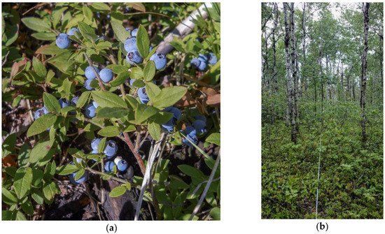
Figure 1.
(a) Velvet-leaf blueberry (Vaccinium myrtilloides Michaux) with ripe fruit from northeast Alberta, Canada; (b) example habitat where blueberry is abundant in the understory, here in a semi-open dry aspen forest (note transect line). Photographs by S.E. Nielsen.
2. Materials and Methods
2.1. Study Species and Study Area
We assessed velvet-leaf blueberry (Figure 1, hereafter, ‘blueberry’) occurrence and abundance over a large region of boreal forest in northeast Alberta, Canada. In Chipewyan, this species is known as tsánlhchoth, and Cree names for this species include inimena, enimina, īyinomin (“person berry”), iynimin, ithīnīmina (“Indian berry”), and sīpīkōmin (from English as “blue berry”) [34]. This species is widely distributed across the northern forests of North America [35]. In the United States this species ranges from New England south through the Appalachian Mountains, to as far south as North Carolina, where it is uncommon and at its lowest latitude. It is widespread throughout the Midwest USA and is especially common in the upper Great Lakes. In the western USA, this species is less common, and restricted to the mountains of northwest Montana and northcentral Washington adjacent to the Canadian border. In Canada, this species of blueberry is distributed throughout most of the forested regions of the country, being present in all provinces, as well as the Northwest Territories, but it is particularly common in boreal forests, and especially in dry upland jack pine (Pinus banksiana Lamb.) and open deciduous and mixed forests [36].
The study took place in the Athabasca region of northeast Alberta, Canada, specifically the region south of Lake Athabasca that borders the province of Saskatchewan on the east, and to the south the southern periphery of the boreal forest that transitions from Crown land to private lands and agriculture (Figure 2). This large area (81,156 km2) comprises a mosaic of boreal peatland and upland forests, with distinct terrain features including the Birch and Stony Mountains [37]. Although called mountains, these features are more correctly considered large plateaus with flat terrain on top that are often dominated by peatlands and with relatively steep sides, especially their eastern flanks. Elevation differences from the base to plateau are moderate at ~200 and ~400 m for the Stony and Birch Mountains, respectively (Figure 2).
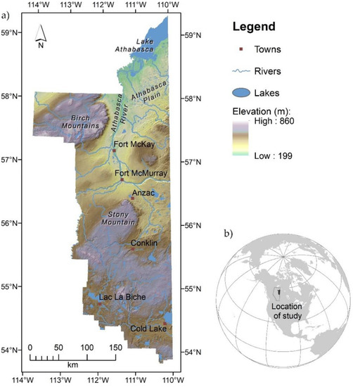
Figure 2.
Terrain, elevation, major water features, and towns within the study area (a); and location of Alberta, Canada (outline) and study area (gray polygon) within North America (b).
The study region contains some of the world’s largest oil reserves: the Athabasca oil sands [37]. Extraction of this resource includes surface mines near Fort McKay where bitumen is near the surface, and more extensive sub-surface mining using a network of small-footprint wells throughout the area, but especially in a zone between Cold Lake in the south and Fort McKay in the north (Figure 2). Many parts of the region are dominated by peatlands [38] wherein forestry is largely absent, but the remaining upland forests are sustainably managed for fiber production (pulp/paper and lumber). Lastly, wildfires are common to the study area, representing the primary natural disturbance, with average fire rotations varying from 167 to 180 years in boreal forests [39], but more frequent in some parts of the region, especially on the Athabasca Plain (Figure 2).
2.2. Study Design and Field Measures for Mapping Blueberry Distribution (Occurrence)
Local occurrence of blueberry was quantified in the field at 845 quarter-hectare (50 × 50 m) plots sampled in the summer months between the years 2012–15 via two sampling campaigns. The first included 510 plots from a regional rare plant study that quantified presence/absence of all vascular plant species within plots (2012–2014) [40]. The second included 335 plots sampled in 2014 and 2015 for the specific purpose of quantifying regional fruiting shrub habitat; these were coded as presence/absence observations for the occurrence portion of this analysis (Appendix A, Figure A1). The former protocol (occurrence plots) involved observers walking belt transects (~2–4 m strip widths) within the 50 × 50 m plots to record all vascular plants [41], including blueberry, whereas the latter (abundance plots) involved a central 50 m transect where shrub abundance and fruit density were measured within sub-plots along the transect. Likewise, the protocol for measuring occurrence within abundance plots included meander surveys within 25 m of each side of the central 50 m transect to document presence/absence of blueberry if it was not detected within the sub-plots used for measuring abundance (see Section 2.3 for details on measures of abundance).
For the 510 plots from the regional rare plant study, plot locations were stratified by model-based estimates of the likelihood of encountering rare vascular plants using a land cover classification raster from Ducks Unlimited (Enhanced Wetland Classification, DU-EWC), and terrain-derived variables from a 50 m digital elevation model (DEM) derived from 1:50,000 Topographic Data of Canada (CanVec series). In contrast, plots for the fruiting shrub project were only stratified by land cover (DU-EWC), but also generally considered time since fire. In both cases, anthropogenic land cover classes were not sampled, nor were aquatic cover types where blueberry cannot grow. Although both sampling campaigns were geographically constrained by the logistics of field sampling (Appendix A, Figure A1), plot locations were representative of major land cover types and regional differences in soils, moisture gradients, and climate. In both cases plots were located in habitats that varied from graminoid rich fens to xeric jack pine forests. For the purposes of modeling species–environment associations, this stratified design ensured a more even sampling distribution in environmental space, rather than geographic space, which is recommended for environmental niche models [42].
2.3. Study Design and Field Measures of Blueberry Shrub Abundance and Fruit Production
In contrast to data used in mapping blueberry distribution (occurrence), shrub abundance, measured as percent shrub cover, and fruit production, measured as counts of fruit (density), were obtained from the 335 abundance plots designed for this purpose (Appendix A, Figure A1a). Specifically, shrub cover and fruit production were measured within a sub-sample of the 0.25 ha plot by first running a 50 m transect on a south-north bearing and dividing that transect into five sequential sub-plots that were 10 m long by 2 m wide (1 m on either side of transect tape). Blueberry shrub cover was then visually estimated in each sub-plot based on ordinal percent cover categories defined as 0 = absent; 1 = <1%; 2 = 1–5%; 3 = 6–25%; 4 = 26–50%; 5 = 51–75%; 6 = 76–95%; and 7 = 96–100%. We used the mid-point value for each sub-plot (assuming 0.1% cover for the “1” cover class), and averaged all sub-plots to obtain a single plot-wide (0.01 ha) measure of cover. Likewise, fruit abundance was measured in the same sub-plots along the same transect, once berries had developed, again using ordinal categories defined here as 0 = none; 1 = <1/m2; 2 = 1–5/m2; 3 = 6–25/m2; 4 = 26–50/m2; 5 = 51–100/m2; 6 = >100/m2. Mid-points of fruit for each sub-plot (assuming 0.1 fruit/1 m2 for “1” and 100 fruit/m2 for the “6”) were then reported for each plot on an average fruit per m2 basis. If fruit abundance was too high to accurately estimate within the larger sub-plots, we used 1 m2 circular quadrats centered within each sub-plot and averaged over the plot.
2.4. Statistical Modeling of Blueberry Occurrence, Abundance, and Fruit Production
We used a conditional or nested approach to modeling occurrence, abundance, and fruit production [16,43]. First, we assessed the occurrence of blueberry shrubs within field plots using logistic regression [44], as is typical for species distribution modeling. This involved the use all 845 quarter-hectare plots from the study area (Appendix A, Figure A1b). Second, we assessed blueberry shrub abundance and fruit production using the 335 sites where cover was measured, but conditional to only those plots where blueberry shrubs were present (n = 186). Although techniques can be used to model occupancy (0 s) and counts (>0) in a single model for situations with excessive zeros (e.g., zero-inflated count models), we find it more efficient to develop individual models for each response, particularly when there are large numbers of explanatory variables that would make model selection difficult. Moreover, factors influencing these processes are expected to differ based on theory and practice [45]. Abundance was represented by mid-point averages of cover scaled to a particular plot size that resulted in continuous cover values, but was bounded between 0% and 100%. Our approach to addressing this was to use fractional logistic regression [46], where cover values were converted to proportions as scaled from the lowest to highest value, and then modeled using a generalized linear model (GLM) with a binomial family, logit link, and the ‘robust’ option [47]. This ensured that predictions for all places in the landscape were not lower or higher than the range of observed values, which is a common problem related to other approaches. Finally, we modeled fruit production, once again using the fractional logistic regression approach, where fruit counts where scaled from 0 to 1 and the same GLM model used as for cover, but here considering only those plots that were at a phenological stage that allowed for fruit counts (n = 90). Model predictions from abundance and fruit production models were then both back-transformed.
We then individually related occurrence, abundance, and fruit production to a suite of environmental, remote sensing, and stand variables (i.e., geospatial data) using each of the model structures. These variables included remotely sensed land cover types from the DU-EWC (15 classes used here), general soil characteristics from the Soil Landscape of Canada version 3.2 [48], terrain-derived variables from a 50 m DEM, and climate variables (Appendix A, Table A1). Climate variables were provided at a resolution of 300 m and rescaled to 50 m using bilinear interpolation. The original DU-EWC had a resolution of 30 m and was rescaled to 50 m using a majority filter, with binary variables created for each land cover class. Soil variables were in polygon format and converted to a 50 m raster. Finally, ALS cloud metrics were processed at a 50 m resolution. Soil variables included soil pH, % sand texture, % clay texture, and soil depth (cm to bedrock). Terrain-derived variables included: a compound topographic index (CTI) representing terrain wetness [49,50]; heatload as it relates to potential solar radiation, weighted to southwest slopes to emphasize afternoon heating [51]; and percent slope (Appendix A, Table A1). Climate variables included mean annual temperature (MAT), mean annual precipitation (MAP), and frost-free period (FFP), all of which were obtained from the ClimateAB model [52].
In addition to the land cover and environmental variables used for all models, the fruit production model included two additional variables: (1) shrub abundance (scaled from 0 to 1), since fruit production should scale with shrub abundance at suitable fruiting sites; and (2) forest canopy cover (percent) derived from ALS data. The ALS data were collected using acquisition standards developed by the Government of Alberta (GOA) [53]. The GOA has been purchasing licensed ALS data on an annual basis since circa 2008. The provincial-scale ALS program has resulted in a dataset with a range of dates, sensor types, and other acquisition parameters, but the adherence to the standard [53] results in a fairly consistent dataset that has been previously used successfully for vegetation analyses [6,40]. The acquisition dates in the study area range from 2007 to 2013, with typical point densities of 1–4 returns/m2. The majority of the ALS data were collected within a few years of when field data were collected. Horizontal cover was defined as the percentage of ALS returns >1.37 m within 50 m pixels, and were processed using FUSION software [54]. Forest canopy cover was square-root transformed since preliminary analyses demonstrated skewed responses and poor fit to untransformed data. An interaction between overstory canopy and shrub cover was tested to examine whether the two factors were additive or multiplicative, since we expected greater shrub cover within open canopy sites could substantially boost fruit production. We also considered the use of a binary ‘dummy’ variable for sampling year (2014 vs. 2015) to account for potential inter-annual variation in fruit production, but no significant difference in fruit counts between years was found; thus, year was not further considered. All statistical modeling was performed in STATA 14 [55].
Model building followed a modified version of the purposeful model building approach [56], whereby variables hypothesized as important were added in a specific sequence and assessed for significance until a final model structure with significant factors (p < 0.1) following the threshold suggested by Hosmer & Lemeshow [57]). Specifically, our approach to model building used local factors first, and then sequentially added variables at larger scales in the order of: (1) land cover, (2) soils, (3) terrain, and (4) climate, except for fruit abundance where we did not consider land cover or climate given the smaller sample size (n = 90), but instead added shrub abundance and forest canopy cover. Variables were added only if uncorrelated (r < |0.7|) and retained only if significant (p < 0.1), excluding land cover variables where we included non-significant cover types along with significant cover types. In some cases, land cover types of similar nature were combined if their responses were comparable or lacking enough field observations in abundance models. Land cover variables used deciduous forest as the reference category, and thus land cover coefficients measure how it differs from deciduous forests. Finally, non-linear effects of climate, soil, and terrain wetness were tested, but only retained in models if significant (Appendix A, Table A1). Model predictive accuracy for the occurrence model was assessed using cross-validation methods via a five-fold randomized assignment of data, wherein 20% of data were iteratively withheld for validation (testing data) and the remaining 80% used for model training. We report the area-under the curve receiver operating characteristic (AUC-ROC) [58] for our full model using all observations, as well as the range of AUC values for the five validation models, whereby any ROC value >0.70 was considered to have good model predictive accuracy [59]. Finally, null models were used to further test whether predicted occurrence differed from what would be expected based on chance [60]. This was done by developing 199 null models that each randomly sampled 845 locations within the study area. Of these, 516 locations were randomly coded as present and the remaining 329 coded as absent to match the prevalence of real data, with a minimum distance between observations of 150 m. ROC values were determined for each null model and compared to the single observed ROC value of the predictive model using a one-sample t-test where rejection of the statistic (one-sided analysis where ROC of the real model > ROC of null models) would indicate our model was significantly better than random chance alone.
2.5. Landscape Predictions of Blueberry Occurrence, Abundance, and Fruit Production
Predictions of species’ occurrence, abundance, and fruit production were mapped using model coefficients and environmental geospatial variables in ESRI ArcGIS version 10.6.1 at a 50 m resolution. Anthropogenic and aquatic land cover types were masked as the species being absent (0). A presence-absence map was then defined by thresholding the probability of occurrence model using a probability cut-off value based on where model sensitivity and specificity values were maximized [58]. The presence-absence map was then used as a mask to constrain predictions of shrub abundance and fruit production, since these responses are conditional to where blueberry was first predicted to be present. Because shrub abundance was used to estimate fruit production, spatial predictions of fruit production used predicted shrub abundance as an input. ALS data on forest canopy cover were available for 83.5% of the study area, and we therefore limited predictions of fruit production to those areas.
2.6. Habitat Enhancements: Effects of Simulated Forest Canopy Removal on Fruit Production
After estimating current fruit production, we examined the potential benefit of removing forest canopy to enhance fruit production in blueberry by simulating reductions in canopy across the region for where ALS data were available (83.5% of the area). Specifically, we quantified the expected gain in fruit production by predicting fruit production under simulated reductions in canopy (to 0%). We then compared the simulated fruit production to their current values through subtraction to estimate the potential gain (change) in fruit supply since fruit production is inversely related to forest canopy cover [18,31,61]. Thus, maps of this change reflect where: (1) blueberry is likely to occur and be abundant (cover), given the environmental constraints that relate to occupancy-abundance; (2) where environmental conditions are suitable for fruit production, but production is limited by forest canopy cover; and (3) where changes in forest canopy cover result in the largest increases in fruit production. Such sites would benefit from overstory disturbances from wildfires, prescribed fires, tree thinning (natural or human-induced), or even forest harvesting if using understory protection. Ultimately defining the most suitable sites for management and habitat enhancements, including habitat offsets that address direct (removal) or indirect (access) losses of the resource.
3. Results
3.1. Landscape Patterns in Blueberry Occurrence
Blueberry shrubs were detected at 516 of the 845 quarter-hectare plots sampled for an overall prevalence of 61.1%. The presence of blueberry shrubs was significantly related to 23 variables. Land cover types represented 16 of those variables, with blueberry occurrence being higher in pine forests, conifer swamps, and conifer forests, and lower in fens, bogs, and shrub-swamps when compared to the deciduous forest reference category (Table A2). Edaphically, occurrence was related non-linearly to soil pH, positively related to the amount of clay and sand in soils (and thus negatively related to percent silt), and more likely in sites with shallow soil depths. Topographically, shrub occurrence was negatively related to percent slope and terrain wetness, pointing to greater likelihood in flat, dry sites. Climate variables were not significantly related to blueberry occurrence. Model predictive accuracy was good at a ROC AUC of 0.78 using all observations (within-model validation), and ranged from 0.77 to 0.80 (mean 0.78) for the five cross-validation models (out-of-model validation). Null model ROC AUC averaged 0.59 (S.D. = 0.02) ranging from a low of 0.55 to a high of 0.63 and was significantly different than the true predictive model (t = −0.018, df = 198, p < 0.001). Optimal cut-off probability for the classification of presence–absence was set at 0.64. Spatially, blueberry presence was predicted to be common throughout the region at an overall prevalence of 48.1% (53.5% when removing water, agriculture, and other masked non-habitat), but noticeably absent in areas of mature deciduous forests in the south near Lac la Biche (Figure 3a,b).
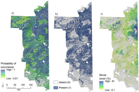
Figure 3.
Predicted probability of occurrence (a), presence (b), and abundance (c) of velvet-leaf blueberry (Vaccinium myrtilloides Michaux) in northeast Alberta, Canada. White areas represent lakes, and grey areas lack native vegetation (agriculture, etc.) in (a) or areas predicted to have no blueberry shrubs (b,c). A digital elevation model-derived hillshade model is used as a base layer in maps to emphasize the underlying terrain.
3.2. Landscape Patterns in Blueberry Shrub Abundance
An abundance of blueberry shrubs, where present, was significantly related to 23 variables (15 being land cover, but grouped into only seven classes) with abundance highest in recently (~10-years) burned sites and treed-rich fens, and lowest in conifer forests, treed-poor fens, bogs, and swamps (Table A2). There were notable differences between land cover relationships for blueberry shrub cover to that of occurrence. For example, pine forests have very high rates of blueberry shrub occurrence (highest prevalence among all land cover types), but shrub abundance was not significantly related to pine forests, which was weakly negative in its effect (relative to deciduous stands). Edaphically, shrub abundance was related non-linearly to the amount of clay in soils and soil depth, with both peaking at low or moderately-high values. Topographically, shrub abundance was inversely related to heatload, and thus abundance increased along northeast-facing slopes. Climatically, shrub abundance was inversely related to mean annual temperature (cooler areas) and non-linearly related to precipitation with areas of increased precipitation generally increasing shrub abundance, but this relationship diminished in the areas of highest precipitation. Spatially, blueberry shrub abundance was predicted to be highest (maximum cover in field plots and maps was 81%) in the region northeast of Fort McMurray, along the Saskatchewan border and the west side of Stony Mountain (Figure 1 and Figure 3c). These areas both experienced large wildfires in the prior decade (see Appendix A, Figure A1). Although blueberry shrubs are among the most common plant species in the boreal forest with prevalence in field plots and landscape predictions >50% for terrestrial habitats, areas of abundant blueberry cover are less common. For example, 11% of occupied sites were predicted to exceed 25% blueberry shrub cover, and only 4% exceeded 50% cover.
3.3. Landscape Patterns in Blueberry Fruit Production
Blueberry fruit production was significantly related to four variables. Not surprisingly, it was positively related to blueberry shrub abundance and inversely related to forest canopy cover (Table 1). Maximum observed fruit production in the field was 53.2 fruit/m2, but highly productive patches were uncommon. Edaphic and terrain factors significantly affected fruit production being inversely related to amount of clay and positively related to southwest slopes as measured by the heatload index. Although one might expect an interactive effect between shrub abundance and forest canopy cover on fruit production, this was not supported (non-significant), pointing to additive, yet non-linear effects due to the square-root transformation of forest canopy cover (Figure 4). When examining predicted responses in fruit to forest canopy and shrub cover, an increase in forest canopy cover from 0% to 100% was predicted to decrease fruit production nearly five-fold, while an increase in shrub cover increased fruit production 3–4-fold (Figure 4).

Table 1.
Model results predicting blueberry fruit production (scaled from 0 to 1) from 90 plots in northeast Alberta, Canada using fractional logistic regression. Model coefficients (β), standard errors (SE), and significance (p) are reported.
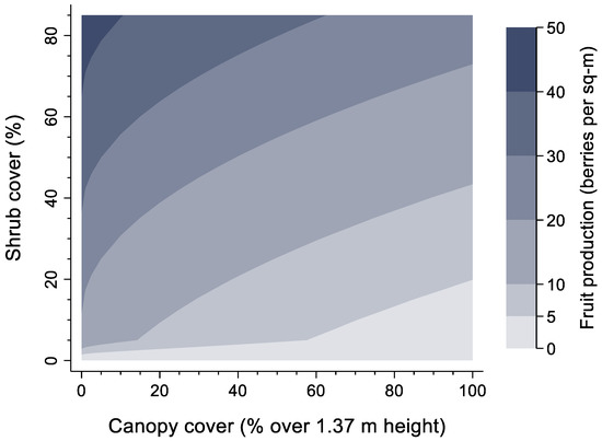
Figure 4.
Predicted average fruit production (berries/m2) of velvet-leaf blueberry as a function of forest canopy cover measured from Airborne Laser Scanning (ALS) data (fraction of first returns at >1.37 m height) and blueberry shrub cover. All other variables were held at their mean.
Figure 4 illustrates the full range of values for both shrub and forest canopy cover and their influence on fruit production holding all other factors at their mean value. The highest possible fruit production was between 40–50 fruit/m2 at sites with maximum shrub cover (81%) and open canopies. Spatially, fruit production was closely related to patterns in shrub cover and thus highest in the areas of predicted high shrub cover, but with significant local modifications due to soils (clay texture), terrain (heatload), and especially local patterns in forest canopy cover measured by ALS (Figure 5). Like that of blueberry shrub cover, sites where fruit are abundant are uncommon despite the species itself being common. For example, 28% of occupied sites were predicted to have fruit production exceeding 10 fruit/m2, while only 11% of occupied sites exceeded 25 fruit/m2.
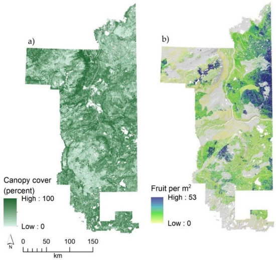
Figure 5.
Velvet-leaf blueberry fruit production based on airborne LiDAR forest canopy cover (fraction of first returns >1.37 m height) (a) and predicted fruit production (fruit/m2) for northeast Alberta, Canada (b). Note that parts of the study area (Cold Lake Air Weapons Range in the southeast; private lands in the south-southwest) did not have LiDAR coverage and thus predictions restricted. A DEM-derived hillshade model is used as a base layer in maps to emphasize the underlying terrain.
3.4. Identifying Priority Sites for Habitat Enhancements
Maps predicting gains in blueberry fruit production with simulated forest canopy thinning (Figure 6) provide a framework for identifying sites for habitat enhancements or simply locations where fruit production should increase most following natural forest disturbances. Overall, some of the greatest gains were predicted to occur over much of the north and east parts of the study area, especially east of the Athabasca River. However, even moderately-high gains were predicted for much of the region where blueberry shrubs are present, suggesting strong ‘top-down’ limitations from overstory canopy and opportunities for improving fruit production with canopy disturbance/thinning. For instance, 42% of current blueberry habitat has the potential to increase their fruit production by 10 fruit/m2 with canopy disturbance to open conditions (0% forest canopy cover), and 14% of this area would exceed 20 fruit/m2. When examining gains in fruit by broad land cover types, the order of greatest to lowest potential gains were in pine forests, deciduous forests, and bogs and fens.
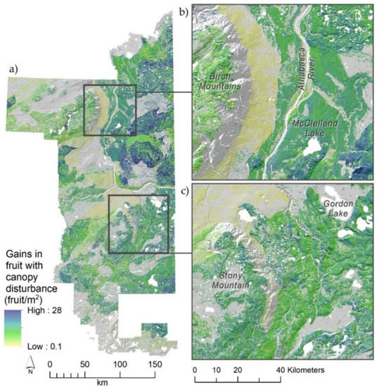
Figure 6.
Predictions of where fruit production would be enhanced most under a scenario of complete forest canopy disturbance (natural, e.g., fires; or management, e.g., tree thinning/removal) (a). Estimates (fruit/m2) were obtained from differences in fruit production predicted under current forest canopy cover (airborne laser scanning returns >1.37 m height) from those expected with canopy disturbance. Sub-panels (b) and (c) provide more detailed illustrations of local responses. A digital elevation model-derived hillshade is used as a base layer in maps to emphasize the underlying terrain.
4. Discussion
Although blueberry is a common boreal species, our results illustrate that areas of abundant shrub cover and high fruit production are much less common and thus of high value. Blueberry shrub occurrence was strongly associated with land cover, specifically jack pine and spruce (Picea spp.) dominated forests, shallow sandy and surprisingly clayey soils, and dry, flat areas. The lack of significant relationships with climactic variables confirms the wide climactic tolerance of this species, consistent with the widespread distribution of the species in Canada and the northern USA. By contrast, abundance was highest in recently burned sites and treed fens, on soils with low to moderate amounts of clay, and shallow to moderate soil depths, in cooler areas and cooler slopes, and areas of moderate to high precipitation. This is a product of differing processes driving occupancy and abundance. Previous work has suggested that local abundance will be related to life history traits, especially clonality, whereas occupancy (range size) is limited by habitat availability [62]. We note that blueberry is capable of extensive clonal reproduction and thus can be long-lived [63], as are many boreal species [64], and our results likely reflect environmental factors driving patterns in vegetative reproduction. Although blueberry can persist under closed-canopies due to plasticity in morphology and biomass allocation, these conditions do not promote sexual reproduction [61], which is ultimately the value of most interest to humans and wildlife.
Assessing fruit production reflects a more targeted management need than does assessing broader patterns in occurrence and abundance. We found that areas of high fruit production were associated with areas of high abundance and were inversely related to forest canopy cover, as measured by ALS data. Although these general relationships are not surprising, little work has been done to quantify their effect sizes and resulting landscape patterns. We did not include land cover and climate variables in fruit production models, but instead found, in contrast to occupancy, that production was negatively associated with clayey soils (i.e., positively correlated with silts and sands), and positively related to ‘warmer’ southwest slopes. In particular, it is evident that even when shrub cover is high, fruit production will be low to moderate without the presence of open forest canopies, illustrating the restrictive additive conditions needed for promoting abundant fruit and highlighting the applicability of using ALS canopy structure measures in modeling fruit production. We did not, however, test other remotely-sensed forest canopy measures, and thus comparisons with ALS are needed to more comprehensively assess its value. These findings also support previous work documenting the general relationship between light availability and fruit production for blueberry and other species of Vaccinium [16,18,61]. For example, Moola [61] documented a nearly 95% increase in blueberry fruit production in a shelterwood cut (partial shade) vs. an overgrown, shaded clearcut (heavy shade). An example from Alaska, United States, demonstrated similar findings at a smaller spatial scale; blueberry shrub abundance was positively related to denser forests (i.e., higher tree densities and basal area), but productivity was negatively related to these sites [18]. Therefore, the authors suggested thinning treatments as a management strategy to increase blueberry yield for Indigenous community harvesting [18].
Habitat enhancements, such as thinning treatments and prescribed burning, can be applied to multiple management goals, for example mitigative offsets to compensate for loss [23], or as resource enhancements for commercial or other purposes [21]. Thinning and forest harvest have been shown to relate to increased blueberry productivity [61,65], as has prescribed burning under open-canopy conditions, for both blueberry and related species [22,66]. Here, we mapped areas that would be most suitable for targeted management of blueberry production through forest canopy opening or would likely relate to increased berry crops following natural disturbance such as wildfire. Specific areas that could be managed to promote major gains in fruit production included those south and east of McClelland Lake, north of Fort McKay at the southern edge of the Athabasca Sand Plain, the eastern slopes of Stony Mountain, and south and east of Anzac, Alberta. Aside from these specific places, nearly all habitats in the region predict gains in blueberry fruit with canopy thinning, suggesting important ‘top down’ limitations in the overstory, as 42% of the area of blueberry increased by 10 fruit/m2. This suggests that although some places will benefit more from canopy removal, many places will respond favorably. The next step in assessing the feasibility and efficacy of the habitat enhancements we suggest would be to compare thinning, both with and without understory protection and via girdling or mechanical removal, as well as prescribed burning treatments.
Access to land in the boreal forest is limited by leases granted to the oil and gas industry. Although these areas remain owned by the Crown, fencing, safety, and access requirements, including expensive training, aesthetics, and the perceived or realized potential for contamination in proximity to resource extraction, effectively limits these areas for public use. Offsets via habitat enhancements could be particularly relevant here since human access to some of these high-quality berry patches will be limited, as was suggested for Alaska blueberry in a similar study promoting Indigenous access to cultural resources [18]. However, we note that berry harvesting patches cannot be regarded as interchangeable given that such places are often tied to ancestral, cultural, and spiritual values [67]. Maps that document important cultural resources, such as berries and medicinal plants, especially those that identify areas for potential enhancements or provide a visual of how reduced access relates to resource losses, can contribute toward food and health sovereignty among Indigenous communities [12,13]. A key next step in developing maps that are useful in representing Indigenous values is to create and include parameters that are meaningful to communities, as demonstrated by Baumflek et al. [12], who included accessibility and travel distance variables determined by community members.
5. Conclusions
Species niche models have wide-ranging applications in ecology, management, and conservation. They broaden our understanding of environmental factors limiting species and processes regulating occurrence and abundance, and can be used to guide management and conservation. Here, we used a fractional logistic regression approach to model velvet-leaf blueberry occurrence, abundance, and fruit production in northeast Alberta, Canada, at high spatial resolution using a suite of remote sensing and other geospatial data. Our study included ALS forest canopy structure data, the application of which we strongly encourage in future studies of understory species, especially fruiting shrubs. Broadly, we observed differences in the environmental factors related to blueberry occurrence, abundance, and productivity that reflect processes such as vegetative reproduction and relationships between light and fruiting. Moreover, our approach of assessing these three ‘dimensions’ of a single species relates to differential management goals over broad scales, and provides a more complete assessment of how this important species relates to measureable environmental factors such as topo-edaphic factors and forest canopy closure. Mapped predictions of blueberry fruit production for the region identified places of current cultural and wildlife value, but also places where productivity gains in fruit would be highest with forest canopy reduction or removal. These places represent areas to target management to enhance accessible blueberry fruit resources, potentially in response to a loss of high-value patches elsewhere. Identifying which of these areas have existing value to Indigenous communities would be highly valuable and could be achieved through community partnership. Maps like what we have shown here may also find application in identifying areas made inaccessible by resource extraction, or those with lost or diminished capacity for harvesting [27] where patches are irreplaceable. Overall, this work provides a suite of tools and a methodological framework for modeling and managing wildlife values and a cultural keystone species.
Author Contributions
Conceptualization, S.E.N.; Methodology, S.E.N. and J.M.D.; Software, S.E.N. and C.W.B.; Validation, S.E.N. and J.M.D.; Formal analysis: S.E.N.; Investigation, S.E.N. and J.M.D.; Resources, S.E.N., J.M.D., and C.W.B.; Data Curation, S.E.N., J.M.D., and C.W.B.; Writing—Original Draft Preparation, S.E.N. and J.M.D.; Writing—Review & Editing, C.W.B.; Visualization, S.E.N. and J.M.D.; Supervision, S.E.N.; Project Administration, S.E.N. and J.M.D.; Funding Acquisition, S.E.N. All authors have read and agree to the published version of the manuscript.
Funding
This research received funding from the Cumulative Effects Management Association (CEMA), the Ecological Monitoring Committee for the Lower Athabasca, Joint Oil Sands Monitoring, Alberta Environmental Monitoring, Evaluation, and Reporting Agency, The Environmental Monitoring and Science Division of Alberta Environment and Parks, and a joint grant from the Natural Sciences and Engineering Research Council (NSERC) and Canada’s Oil Sands Innovation Alliance (COSIA) as Grant #: CRDPJ 498955-16 (Nielsen).
Acknowledgments
Ducks Unlimited provided in-kind support by making available the Enhanced Wetland Classification of the Lower Athabasca.
Conflicts of Interest
The authors declare no conflict of interest. Project funders had no role in the design of the study; in the collection, analyses, or interpretation of data; in the writing of the manuscript, and in the decision to publish the results.
Appendix A
Table A1 and Table A2 contain additional supporting information on model results describing blueberry occurrence, abundance, and fruit production.
Table A1.
List of environmental variables used for modeling blueberry shrub distribution, abundance, and fruit production. Note that the forest canopy cover variable was only used for modeling fruit production and that some variables were tested for non-linear responses using quadratic models as indicated by *. DU-Enhanced Wetland Classification of land cover types were provided at a resolution of 30 m and rescaled to 50 m using a majority filter. Soil Landscapes of Canada was polygon-based and thus converted to a raster at a 50 m resolution. Terrain variables were derived from a 50 m DEM, while ClimateAB variables were re-scaled to 50 m from a 300 m model using bilinear interpolation. Airborne Laser Scanning data were processed for this study at a 50 m resolution.
| Variable | Description | Data Source |
|---|---|---|
| Land cover | (used as binary categories) | |
| Marsh | Land cover of marsh | DU-Enhanced Wetland Classification |
| Fen-G-R | Land cover of fen-graminoid-rich | DU-Enhanced Wetland Classification |
| Fen-G-P | Land cover of fen-graminoid-poor | DU-Enhanced Wetland Classification |
| Fen-S-R | Land cover of fen-shrub-rich | DU-Enhanced Wetland Classification |
| Fen-S-P | Land cover of fen-shrub-poor | DU-Enhanced Wetland Classification |
| Fen-T-P | Land cover of fen-treed-poor | DU-Enhanced Wetland Classification |
| Bog | Land cover of bog | DU-Enhanced Wetland Classification |
| Bog-treed | Land cover of bog-treed | DU-Enhanced Wetland Classification |
| Swamp-S | Land cover of swamp-shrub | DU-Enhanced Wetland Classification |
| Swamp-D | Land cover of swamp-deciduous | DU-Enhanced Wetland Classification |
| Swamp-T | Land cover of swamp-tamarack | DU-Enhanced Wetland Classification |
| Swamp-C | Land cover of swamp-conifer | DU-Enhanced Wetland Classification |
| Decid | Land cover of upland-deciduous | DU-Enhanced Wetland Classification |
| Conifer | Land cover of upland-conifer, not pine | DU-Enhanced Wetland Classification |
| Pine | Land cover of upland-pine | DU-Enhanced Wetland Classification |
| Burn | Land cover of recently burned | DU-Enhanced Wetland Classification |
| Soils | ||
| pH * | Soil pH | Soil Landscapes of Canada v3.2 |
| Clay * | Soil texture, percent clay | Soil Landscapes of Canada v3.2 |
| Sand * | Soil texture, percent sand | Soil Landscapes of Canada v3.2 |
| Depth * | Soil depth (cm) | Soil Landscapes of Canada v3.2 |
| Terrain | ||
| Slope | Percent slope | DEM, derived product (this study) |
| Wetness * | Terrain wetness (CTI method) | DEM, derived product (this study) |
| Heatload | Heatload index | DEM, derived product (this study) |
| Climate | ||
| MAT * | Mean annual temperature (°C) | ClimateAB |
| MAP * | Mean annual precipitation (mm) | ClimateAB |
| FFP | Frost free period (days) | ClimateAB |
| Forest canopy cover | ||
| Canopy | Percent forest canopy cover | Airborne Laser Scanning (this study) |
Table A2.
Model results describing blueberry shrub occurrence using logistic regression and shrub abundance using fractional logistic regression. Model coefficients (β), standard errors (SE), and significance (p) reported for each model. Significant variables (p < 0.1) have parameters in bold font. Note the same values for some fens and bog/swamps in abundance models as those land cover categories were combined and fit as single variables.
| Occurrence | Abundance | |||||
|---|---|---|---|---|---|---|
| Variable | β | SE | p | β | SE | p |
| Land cover | ||||||
| Marsh | −0.412 | 0.751 | 0.583 | |||
| Fen-G-R | −1.682 | 0.569 | 0.003 | 0.197 | 0.958 | 0.837 |
| Fen-G-P | −1.930 | 0.827 | 0.020 | 0.197 | 0.958 | 0.837 |
| Fen-S-R | −0.621 | 0.395 | 0.116 | 0.197 | 0.958 | 0.837 |
| Fen-S-P | −2.959 | 0.779 | 0.001 | 0.197 | 0.958 | 0.837 |
| Fen-T-R | −0.079 | 0.344 | 0.818 | 0.627 | 0.320 | 0.050 |
| Fen-T-P | −0.497 | 0.311 | 0.110 | −1.222 | 0.707 | 0.084 |
| Bog | −0.927 | 0.939 | 0.323 | −0.824 | 0.367 | 0.025 |
| Bog-T | −0.883 | 0.457 | 0.053 | −0.824 | 0.367 | 0.025 |
| Swamp-S | −1.040 | 0.611 | 0.089 | −0.824 | 0.367 | 0.025 |
| Swamp-D | −1.497 | 0.934 | 0.109 | −0.824 | 0.367 | 0.025 |
| Swamp-T | 14.48 | 682.1 | 0.983 | −0.824 | 0.367 | 0.025 |
| Swamp-C | 0.858 | 0.467 | 0.066 | −0.824 | 0.367 | 0.025 |
| Conifer | 0.674 | 0.267 | 0.012 | −1.329 | 0.298 | 0.001 |
| Pine | 0.866 | 0.273 | 0.002 | −0.344 | 0.272 | 0.205 |
| Burn | 1.581 | 1.071 | 0.140 | 1.962 | 0.655 | 0.003 |
| Soil | ||||||
| pH | −4.830 | 2.025 | 0.017 | |||
| pH2 | 0.460 | 0.207 | 0.027 | |||
| Clay | 0.019 | 0.008 | 0.023 | −0.194 | 0.054 | 0.001 |
| Clay2 | 0.003 | 0.001 | 0.001 | |||
| Sand | 0.019 | 0.004 | 0.001 | |||
| Depth | −0.011 | 0.004 | 0.002 | −0.076 | 0.020 | 0.001 |
| Depth2 | 0.0014 | 0.0003 | 0.001 | |||
| Terrain | ||||||
| Wetness | −0.198 | 0.054 | 0.001 | |||
| Slope | −0.389 | 0.085 | 0.001 | |||
| Heatload | −0.005 | 0.002 | 0.014 | |||
| Climate | ||||||
| MAT | −2.296 | 0.706 | 0.001 | |||
| MAP | 0.176 | 0.101 | 0.083 | |||
| MAP2 | −0.0002 | 0.0001 | 0.087 | |||
| Constant | 14.657 | 4.553 | 0.001 | −38.765 | 25.120 | 0.123 |

Figure A1.
(a) Distribution of study plots by type of data collected with ‘occurrence’ plots (n = 510) only assessing presence−absence, while abundance plots (n = 335) assessed presence−absence, shrub abundance where present, and for a subset of plots (n = 90) fruit production for velvet−leaf blueberry in northeast Alberta, Canada; and (b) the distribution (presence−absence) of velvet−leaf blueberry. Broad land cover types are provided in both maps based on the Ducks Unlimited Enhanced Wetland Classification. A DEM−derived hillshade model is used as a base layer in maps to emphasize the underlying terrain.
References
- Lefsky, M.; Cohen, W.; Parker, G.; Harding, D. Lidar remote sensing for ecosystem studies. Bioscience 2002, 52, 19–30. [Google Scholar] [CrossRef]
- Guisan, A.; Thuiller, W. Predicting species distribution: Offering more than simple habitat models. Ecol. Lett. 2005, 8, 993–1009. [Google Scholar] [CrossRef]
- Franklin, J. Predictive vegetation mapping: Geographic modelling of biospatial patterns in relation to environmental gradients. Prog. Phys. Geogr. 1995, 19, 474–499. [Google Scholar] [CrossRef]
- Blanco, J.A.; Ameztegui, A.; Rodriguez, F. Modelling Forest Ecosystems: A crossroad between scales, techniques, and applications. Ecol. Model. 2020, 425, 109030. [Google Scholar] [CrossRef]
- Vauhkonen, J. Predicting the provisioning potential of forest ecosystem services using airborne laser scanning data and forest resource maps. For. Ecosyst. 2018, 5, 1–19. [Google Scholar] [CrossRef]
- Mao, L.; Dennett, J.; Bater, C.W.; Tompalski, P.; Coops, N.C.; Farr, D.; Kohler, M.; White, B.; Stadt, J.J.; Nielsen, S.E. Using airborne laser scanning to predict plant species richness and assess conservation threats in the oil sands region of Alberta’s boreal forest. For. Ecol. Manag. 2018, 409, 29–37. [Google Scholar] [CrossRef]
- Thers, H.; Kirstine, A.; Læssøe, T.; Ejrnæs, R.; Klith, P.; Svenning, J.-C. Lidar-derived variables as a proxy for fungal species richness and composition in temperate Northern Europe. Remote Sens. Environ. 2017, 200, 102–113. [Google Scholar] [CrossRef]
- Guo, X.; Coops, N.C.; Tompalski, P.; Nielsen, S.E.; Bater, C.W.; Stadt, J.J. Regional mapping of vegetation structure for biodiversity monitoring using airborne lidar data. Ecol. Inform. 2017, 38, 50–61. [Google Scholar] [CrossRef]
- Nielsen, S.E.; Mcdermid, G.; Stenhouse, G.B.; Boyce, M.S. Dynamic wildlife habitat models: Seasonal foods and mortality risk predict occupancy-abundance and habitat selection in grizzly bears. Biol. Conserv. 2010, 143, 1623–1634. [Google Scholar] [CrossRef]
- Pollock, S.Z.; Nielsen, S.E.; St. Clair, C.C. A railway increases the abundance and accelerates the phenology of bear-attracting plants in a forested, mountain park. Ecosphere 2017, 8. [Google Scholar] [CrossRef]
- Questad, E.J.; Kellner, J.R.; Kinney, K.; Cordell, S.; Asner, G.P.; Thaxton, J.; Diep, J.; Uowolo, A.; Brooks, S.; Inman-Narahari, N.; et al. Mapping habitat suitability for at-risk plant species and its implications for restoration and reintroduction. Ecol. Appl. 2014, 24, 385–395. [Google Scholar] [CrossRef]
- Baumflek, M.; DeGloria, S.; Kassam, K.A. Habitat modeling for health sovereignty: Increasing indigenous access to medicinal plants in northern Maine, USA. Appl. Geogr. 2015, 56, 83–94. [Google Scholar] [CrossRef]
- Gaikwad, J.; Wilson, P.D.; Ranganathan, S. Ecological niche modeling of customary medicinal plant species used by Australian Aborigines to identify species-rich and culturally valuable areas for conservation. Ecol. Model. 2011, 222, 3437–3443. [Google Scholar] [CrossRef]
- Kangas, K.; Markkanen, P. Factors affecting participation in wild berry picking by rural and urban dwellers. Silva Fenn. 2001, 35, 487–495. [Google Scholar] [CrossRef]
- Kuhnlein, H.V.; Turner, N.J. Traditional Plant Foods of Canadian Indigenous Peoples; Gordon and Breach Science: Amsterdam, The Netherlands, 1991. [Google Scholar]
- Barber, Q.E.; Bater, C.W.; Braid, A.C.R.; Coops, N.C.; Tompalski, P.; Nielsen, S.E. Airborne laser scanning for modelling understory shrub abundance and productivity. For. Ecol. Manag. 2016, 377, 46–54. [Google Scholar] [CrossRef]
- Gopalakrishnan, R.; Thomas, V.A.; Wynne, R.H.; Coulston, J.W.; Fox, T.R. Shrub detection using disparate airborne laser scanning acquisitions over varied forest cover types. Int. J. Remote Sens. 2018, 39, 1220–1242. [Google Scholar] [CrossRef]
- Reich, R.M.; Lojewski, N.; Lundquist, J.E.; Bravo, V.A. Predicting abundance and productivity of blueberry plants under insect defoliation in Alaska. J. Sustain. For. 2018, 37, 525–536. [Google Scholar] [CrossRef]
- Franklin, C.M.A.; Nielsen, S.E.; Macdonald, S.E. Understory vascular plant responses to retention harvesting with and without prescribed fire. Can. J. For. Res. 2019, 49, 1087–1100. [Google Scholar] [CrossRef]
- Koivula, M.; Vanha-Majamaa, I. Experimental evidence on biodiversity impacts of variable retention forestry, prescribed burning, and deadwood manipulation in Fennoscandia. Ecol. Process. 2020, 9, 1–22. [Google Scholar] [CrossRef]
- Granath, G.; Kouki, J.; Johnson, S.; Heikkala, O.; Rodríguez, A.; Strengbom, J. Trade-offs in berry production and biodiversity under prescribed burning and retention regimes in boreal forests. J. Appl. Ecol. 2018, 55, 1658–1667. [Google Scholar] [CrossRef]
- Duchesne, L.C.; Wetzel, S. Effect of Fire Intensity and Depth of Burn on Lowbush Blueberry, Vaccinium angustifolium, and Velvet Leaf Blueberry, Vaccinium myrtilloides, Production in Eastern Ontario. Can. Field-Nat. 2004, 118, 195–200. [Google Scholar] [CrossRef]
- Braid, A.C.R.; Manzer, D.; Nielsen, S.E. Wildlife habitat enhancements for grizzly bears: Survival rates of planted fruiting shrubs in forest harvests. For. Ecol. Manag. 2016, 369, 144–154. [Google Scholar] [CrossRef]
- Roberts, D.R.; Nielsen, S.E.; Stenhouse, G.B. Idiosyncratic responses of grizzly bear habitat to climate change based on projected food resource changes. Ecol. Appl. 2014, 24, 1144–1154. [Google Scholar] [CrossRef]
- Garibaldi, A. Moving from model to application: Cultural keystone species and reclamation in Fort McKay, Alberta. J. Ethnobiol. 2009, 29, 323–338. [Google Scholar] [CrossRef]
- Golzadeh, N.; Barst, B.D.; Basu, N.; Baker, J.M.; Auger, J.C.; McKinney, M.A. Evaluating the concentrations of total mercury, methylmercury, selenium, and selenium:mercury molar ratios in traditional foods of the Bigstone Cree in Alberta, Canada. Chemosphere 2020, 250, 126285. [Google Scholar] [CrossRef] [PubMed]
- Baker, J.M. Do berries listen? Berries as indicators, ancestors, and agents in Canada’s Oil Sands Region. Ethnos 2020. [Google Scholar] [CrossRef]
- Jarron, L.R.; Coops, N.C.; Mackenzie, W.H.; Tompalski, P.; Dykstra, P. Detection of sub-canopy forest structure using airborne LiDAR. Remote Sens. Environ. 2020, 244, 111770. [Google Scholar] [CrossRef]
- Berkes, F.; Davidson-Hunt, I.J. Biodiversity, traditional management systems, and cultural landscapes: Examples from the boreal forest of Canada. Int. Soc. Sci. J. 2006, 58, 35–47. [Google Scholar] [CrossRef]
- Seeram, N.P. Berry fruits: Compositional elements, biochemical activities, and the impact of their intake on human health, performance, and disease. J. Agric. Food Chem. 2008, 56, 627–629. [Google Scholar] [CrossRef] [PubMed]
- Nielsen, S.E.; Munro, R.H.M.; Bainbridge, E.L.; Stenhouse, G.B.; Boyce, M.S. Grizzly bears and forestry II. Distribution of grizzly bear foods in clearcuts of west-central Alberta, Canada. For. Ecol. Manag. 2004, 199, 67–82. [Google Scholar] [CrossRef]
- Garibaldi, A.; Straker, J. Cultural keystone species in oil sands mine reclamation, Fort McKay, Alberta, Canada. In Proceedings of the British Columbia Mine Reclamation Symposium. University of British Columbia Library, Cranbrook, BC, Canada, 14–17 September 2009. [Google Scholar]
- Garibaldi, A.; Turner, N. Cultural keystone species: Implications for ecological conservation and restoration. Ecol. Soc. 2004, 9. [Google Scholar] [CrossRef]
- Marles, R.; Clavelle, C.; Monteleone, L.; Tays, N.; Burns, D. Aboriginal Plant Use in Canada’s Northwest Boreal Forest; Natural Resources Canada: Edmonton, AB, Canada, 2012. [Google Scholar]
- Kloet, V. The Genus Vaccinium in North America; Agriculture Canada Research Branch: Ottawa, ON, Canada, 1988. [Google Scholar]
- Smith, D.W. Ecological studies of Vaccinium species in Alberta. Can. J. Plant Sci. 1962, 82–90. [Google Scholar] [CrossRef]
- Alberta Environment and Sustainable Resource Development. Regional Forest Landscape Assessment—Lower Athabasca Region; Alberta Environment and Sustainable Resource Development: Edmonton, AB, Canada, 2012. [Google Scholar]
- Raine, M.; Mackenzie, I.; Gilchrist, I. CNRL Horizon Project Environmental Impact Assessment; Wetlands and Forest Resources Baseline: Calgary, AB, Canada, 2002; Volume 6. [Google Scholar]
- de Groot, W.J.; Flannigan, M.D.; Cantin, A.S. Climate change impacts on boreal fire regimes. For. Ecol. Manag. 2013, 294, 35–44. [Google Scholar] [CrossRef]
- Nielsen, S.E.; Dennett, J.M.; Bater, C.W. Landscape patterns of rare vascular plants in the Lower Athabasca. Forests 2020, 11, 699. [Google Scholar] [CrossRef]
- Zhang, J.; Nielsen, S.E.; Grainger, T.N.; Kohler, M.; Chipchar, T.; Farr, D.R. Sampling plant diversity and rarity at landscape scales: Importance of sampling time in species detectability. PLoS ONE 2014, 9, e95334. [Google Scholar] [CrossRef]
- Peterson, A.T.; Soberon, J.; Pearson, R.G.; Anderson, R.P.; Martinez-Meyer, E.; Nakamura, M.; Araujo, M.B. Ecological Niches and Geographic Distributions; Princeton University Press: Princeton, NJ, USA, 2011. [Google Scholar]
- Nielsen, S.E. Fruiting Shrubs of the Lower Athabasca: Distribution, Ecology and a Digital Atlas; ACE-Lab: Edmonton, AB, Canada, 2016; p. 81. [Google Scholar]
- Hosmer, D.W.; Lemeshow, S. Applied Logistic Regression, 2nd ed.; John Wiley & Sons, Inc.: Hoboken, NJ, USA, 2000. [Google Scholar] [CrossRef]
- Nielsen, S.E.; Johnson, C.J.; Heard, D.C.; Boyce, M.S.; Nielsen, S.E.; Johnson, C.J.; Heard, D.C.; Boyce, M.S. Can models of presence-absence be used to scale abundance? Two case studies considering extremes in life history. Ecography 2005, 28, 197–208. [Google Scholar] [CrossRef]
- Baum, C.F. Modeling proportions. STATA J. 2008, 8, 299–303. [Google Scholar] [CrossRef]
- Papke, L.E.; Wooldridge, J.M. Econometric methods for fractional response variables with an application to 401(k) plan participation rates. J. Appl. Econom. 1996, 11, 619–632. [Google Scholar] [CrossRef]
- Soil Landscapes of Canada Working Group. Available online: https://open.canada.ca/data/en/dataset/5ad5e20c-f2bb-497d-a2a2-440eec6e10cd (accessed on 1 September 2010).
- Evans, J. CTI.aml Compound Topographic Index AML Script 2004. Available online: http://arcscripts.esri.com/details.asp?dbid=11863 (accessed on 1 September 2010).
- Jenness, J. Topographic Position Index (tpi_jen.avx) Extension for ArcView 3.x, v. 1.2. 2006. Available online: http://www.jennessent.com/arcview/tpi.htm (accessed on 1 September 2010).
- McCune, B. Improved estimates of incident radiation and heat load using non-parametric regression against topographic variables. J. Veg. Sci. 2007, 18, 751–754. [Google Scholar] [CrossRef]
- Mbogga, M.S.; Hansen, C.; Wang, T.; Hamann, A. A Comprehensive Set of Interpolated Climate Data for Alberta; 2010. Available online: https://open.alberta.ca/publications/9780778591849 (accessed on 1 September 2010).
- Environment and Sustainable Resource Environment. General Specifications for the Acquisition of Lidar Data; Informatics Branch, Government of Alberta: Edmonton, AB, Canada; p. 52.
- McGaughey, R. FUSION/LVD: Software for LIDAR Data Analysis and Visualization 2016. Available online: http://forsys.cfr.washington.edu/FUSION/fusion_overview.html (accessed on 1 July 2010).
- StataCorp Stata Statistical Software: Release 14 2015. Available online: www.stata.com (accessed on 1 July 2010).
- Bursac, Z.; Gauss, C.H.; Williams, D.K.; Hosmer, D.W. Purposeful selection of variables in logistic regression. Source Code Biol. Med. 2008, 3, 17. [Google Scholar] [CrossRef]
- Lemeshow, S.; Hosmer, D.W. A review of goodness of fit statistics for use in the development of logistic regression models. Am. J. Epidemiol. 1982, 115, 92–106. [Google Scholar] [CrossRef] [PubMed]
- Manel, S.; Williams, H.; Ormerod, S. Evaluating presence-absence models in diversity on the roof of the world: Spatial patterns and environmental determinants. J. Appl. Ecol. 2001, 38, 921–931. [Google Scholar] [CrossRef]
- Swets, J. Measuring the accuracy of diagnostic systems. Science 1988, 240, 1285–1293. [Google Scholar] [CrossRef] [PubMed]
- Raes, N.; ter Steege, H. A null-model for significance testing of presence-only species distribution models. Ecography 2007, 30, 727–736. [Google Scholar] [CrossRef]
- Moola, F.M. Yield and Morphological Responses of Wild Blueberry (Vaccinium spp.) to Forest Harvesting and Conifer Release Treatments. Master’s Thesis, Lakehead University, Thunder Bay, ON, Canada, 1997. [Google Scholar]
- Kolb, A.; Barsch, F.; Diekmann, M. Determinants of local abundance and range size in forest vascular plants. Glob. Ecol. Biogeogr. 2006, 15, 237–247. [Google Scholar] [CrossRef]
- Flora of North America Editorial Committee. Flora of North America North of Mexico; Flora of North America Editorial Committee: New York, NY, USA, 1993. [Google Scholar]
- Okland, R.H. Persistence of vascular plants in a Norwegian boreal coniferous forest. Ecography 1995, 18, 3–14. [Google Scholar] [CrossRef]
- Strengbom, J.; Axelsson, E.P.; Lundmark, T.; Nordin, A. Trade-offs in the multi-use potential of managed boreal forests. J. Appl. Ecol. 2018, 55, 958–966. [Google Scholar] [CrossRef]
- Penney, B.G.; McRae, K.B.; Rayment, A.F. Long-term effects of burn-pruning on lowbush blueberry (Vaccinium angustifolium Ait.) production. Can. J. Plant Sci. 1997, 77, 421–425. [Google Scholar] [CrossRef]
- Michell, H.J. Gathering berries in northern contexts: A Woodlands Cree metaphor for community-based research. Pimatisiwin 2009, 7, 65–73. [Google Scholar]
© 2020 by the authors. Licensee MDPI, Basel, Switzerland. This article is an open access article distributed under the terms and conditions of the Creative Commons Attribution (CC BY) license (http://creativecommons.org/licenses/by/4.0/).