Biomass and Volume Modeling along with Carbon Concentration Variations of Short-Rotation Poplar Plantations

Abstract

Short-rotation forestry is of interest to provide biomass for bioenergy and act as a carbon sink to mitigate global warming. The Poplar tree (Populus × xiaohei) is a fast-growing and high-yielding tree species in Northeast China. In this study, a total of 128 Populus × xiaohei trees from the Songnen Plain, Heilongjiang Province, Northeastern China, were harvested. Several available independent variables, such as tree diameter at breast height (D), tree’s total height (H), crown width (CW), and crown length (CL), were differently combined to develop three additive biomass model systems and eight stem volume models for Populus × xiaohei tree. Variance explained within the three additive biomass model systems ranged from 83% to 98%, which was lowest for the foliage models, and highest for the stem biomass models. Similar findings were found in the stem volume models, in which the models explained more than 94% of the variance. The additional predictors, such as H, CL, or CW, evidently enhanced the model fitting and performance for the total and components biomass along with the stem volume models. Furthermore, the biomass conversion and expansion factors (BCEF_s) of the root (118.2 kg/m³), stem (380.2 kg/m³), branch (90.7 kg/m³), and foliage (31.2 kg/m³) were also calculated. The carbon concentrations of Populus × xiaohei in root, stem, branch, and foliage components were 45.98%, 47.74%, 48.32%, and 48.46%, respectively. Overall, the newly established models in this study provided complete and comprehensive tools for quantifying the biomass and stem volume of Populus × xiaohei, which might be essential to be specifically utilized in the Chinese National Forest Inventory.

1. Introduction

Short-rotation forests pertain to plantations of certain fast-growing tree species and harvests continually at a brief period of rotations, which is possible due to the implementation of high planting density and intensive forest management [1,2]. These types of plantations have various objectives, such as alleviating the contradiction between ecology and economy, estimating carbon accumulation, shortening the cycle of timber production management, prompting to produce biomass for bioenergy production, and providing the material for the production of wood pulp, feed, and biomass fuels by short-rotation management [3,4,5,6,7]. Not surprisingly, then, many researchers worldwide are exploring the biomass production potentials of fast-growing tree species [6,7,8,9]. Poplar is one of the most important tree species on earth due to its fast growth, strong adaptability, easy reproduction, and extensive use; thus, it is widely used to produce energy, fuelwood, pulp, and agricultural protection forests in China [10,11].

Populus × xiaohei is currently the most widely cultivated poplar tree, ranging from the northeast to the central areas of China [12,13]. It is commonly used to establish high-yielding and short-rotation plantation forests, and it is one of the primary protection forests and timber species in the Songnen Plain of China. The area and stand volume of Populus × xiaohei plantation forests in the Songnen Plain of China is about 550,000 ha and 52,000,000 cubic meters, respectively [14]. At present, many researchers have strengthened their focus on transgenic technology, growth dynamic, and physiological and ecological characteristics for the biomass of Populus × xiaohei [12,13,15,16,17,18]. Unfortunately, the available information regarding this species’ potential is still inadequate, and only a limited number of studies have been reported about the estimation of its biomass, carbon, and volume production. The in-depth knowledge of this species’ ability to accumulate biomass and volume is necessary to reveal the variation rules of the ecological system balance, and to assess the carbon storage, nutrient cycle, and energy flow. Thus, the production of biomass and volume from Populus × xiaohei, mainly the aim of the Populus × xiaohei forests, should also be considered and evaluated.

As it has been known, directly measuring the stem volume and weights of the tree components are undeniably the most precise approach for estimating individual tree biomass [19,20]. Thus, biomass is often estimated by utilizing the biomass allometric equations or merely by multiplying the stem volume approximations with biomass conversion and expansion factors ($BCE{F}_s$) or basic wood density [13,21,22,23,24,25]. The $BCE{F}_s$ would be more favorable in case the tree volume is the only existing data; thus, it is possible to convert the stem volume data into the tree components’ (i.e., root, stem, branch, and foliage) dry biomass [26,27]. However, utilizing the biomass and stem volume equations are still considered as a better way of quantifying forest biomass and volume [21,23,28]. To date, a considerable amount of volume and biomass models for various tree species have been developed across numerous geographical and ecological regions globally [29,30,31,32,33,34].

The vast majority of the established biomass equations utilize diameter at breast height ($D$) as a sole predictor of tree components’ biomass or stem volume equations [13,21,24,34,35,36]. Furthermore, numerous studies have shown that adding the tree’s total height ($H$) as a predictor in both of components biomass and stem volume equation could significantly upgrade the quality of the model fitting and performance, and it was found to be helpful in explaining the potential limitation of intra-species divergence [23,29,37,38]. Thus, many studies preferred to use $H$ as the second predictor to develop biomass or stem volume models [38,39]. In addition, depending on the research orientations, the tree crown (e.g., crown width [$CW$] and crown length [$CL$]) is also considered as prospective additional independent variables to develop an individual tree biomass model [38,40].

When establishing models to predict the total biomass and that of several primary tree tissues, two definite attributes are widely known as an outcome of employing several different approaches in the model’s fitting process, namely: non-additive and additive models [22]. The non-additive model individually fits the data of each tree tissue and total biomass, neglecting the inherent correlation between the tissues measured on the same sample trees. On the contrary, the additive models require the tree tissues and total biomass data to be simultaneously fitted, reckoning the intrinsic correlation of the biomass tissues sampled from the same individuals [22,37,41]. Consequently, the total tree biomass estimation will be equal to the sum of the prediction of biomass tissues. Over an extended period, researchers have been proposing several methods of biomass model systems in order to deal with the naturally existing additivity property [37,42]. Between these techniques, nonlinear seemingly unrelated regression (NSUR) is acknowledged as one of the most commonly used compared to others, due to its generality and flexibility in application [22].

There are more than 100 poplar species worldwide, and roughly half of them are native to China [11]. Numerous studies about poplar biomass and carbon storage in China were conducted over the last 30 years, but only a few studies reported on biomass and carbon estimations of Populus × xiaohei. Fan et al. [43] and Song et al. [44] studied the biomass allometric relationship of Populus × xiaohei and established the equations to predict the tree components and total biomass. Nevertheless, these two studies only utilized a relatively small biomass dataset, and unfortunately, the compatibility property was absent in the equations developed by Fan et al. [43]. Furthermore, a carbon concentration was usually used to calculate tree carbon. Generally, researchers employ either 50% or 45% as generic carbon concentration values for different tree components [45,46].

However, a range of 43%–60% on tree carbon concentration was reported by several previous studies varying across the tree species and tissues [47,48]. Thus, the usage of the 50% carbon conversion factor might generate a 15% bias in estimating the carbon stock of an individual tree. Considering the potential of Populus × xiaohei tree in global climate change, carbon cycle, carbon storage, and emission reduction, this work intends to consider allometric equations as supplementary instruments for biomass and volumes estimation of this particular species. The specific purposes of the current study were to: (1) construct three additive biomass model systems with weighted NSUR and eight stem volume models based on different combination of predictors; (2) examine the performance of the newly developed biomass and stem volume models; (3) compare the current study’s newly developed biomass and stem volume equations against the previously established biomass and stem volume models for Populus × xiaohei by Fan et al. [43], Song et al. [44], and Yang et al. [49].

2. Materials and Methods

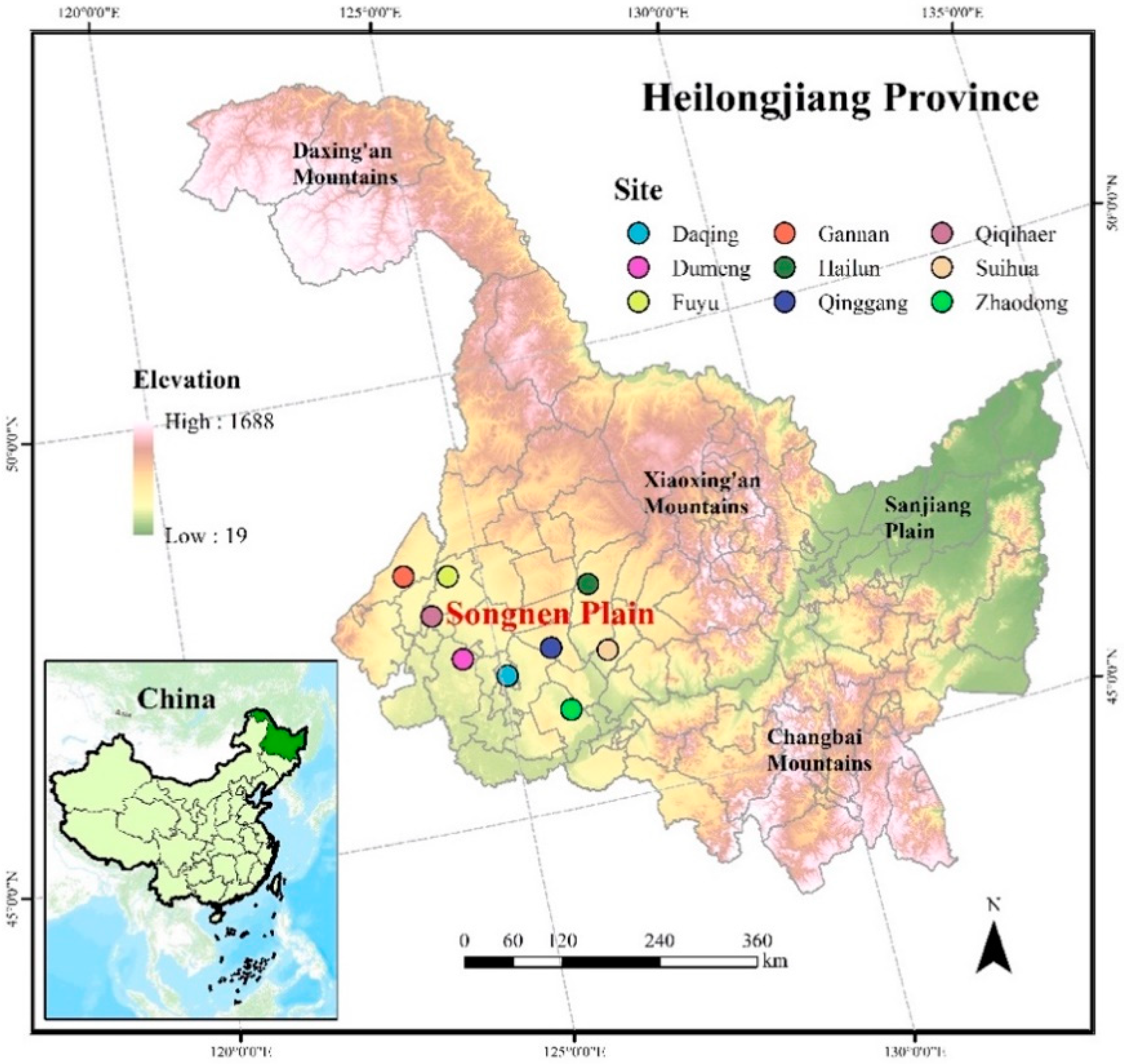
2.1. Site Description

The dataset was obtained from the Songnen Plain of Heilongjiang Province (HSP) (121–128° E, 42–51° N, Figure 1), the largest part amongst the Northeastern Plain region in the People’s Republic of China. It has an area of 12 × 10⁴ km² and is connected with the Xiaoxing’an Mountains in the north, bordered by the Eastern Mountains and the Daxing’an Mountains in the east and west, respectively (Figure 1). The elevation ranges between 120 and 300 m above sea level. The HSP has a semi-humid continental monsoon climate and is located in a warm temperate zone. The mean daily air temperature in January and July is −20 °C and +25 °C, respectively. The mean temperature and annual rainfall are around 2–6 °C and about 500 mm, respectively. The soil types in the HSP are mostly Chernozem (Pachic Haploboroll) and black soil (Pachic Udic Argiboroll), according to the Chinese Taxonomic System. The HSP is dominated by herbaceous vegetation with a small number of trees and shrubs. The tree layer is mainly covered by planted forest with Populus × xiaohei as the dominant tree species and considered to be the best choice for windbreaks.

2.2. Data Collection

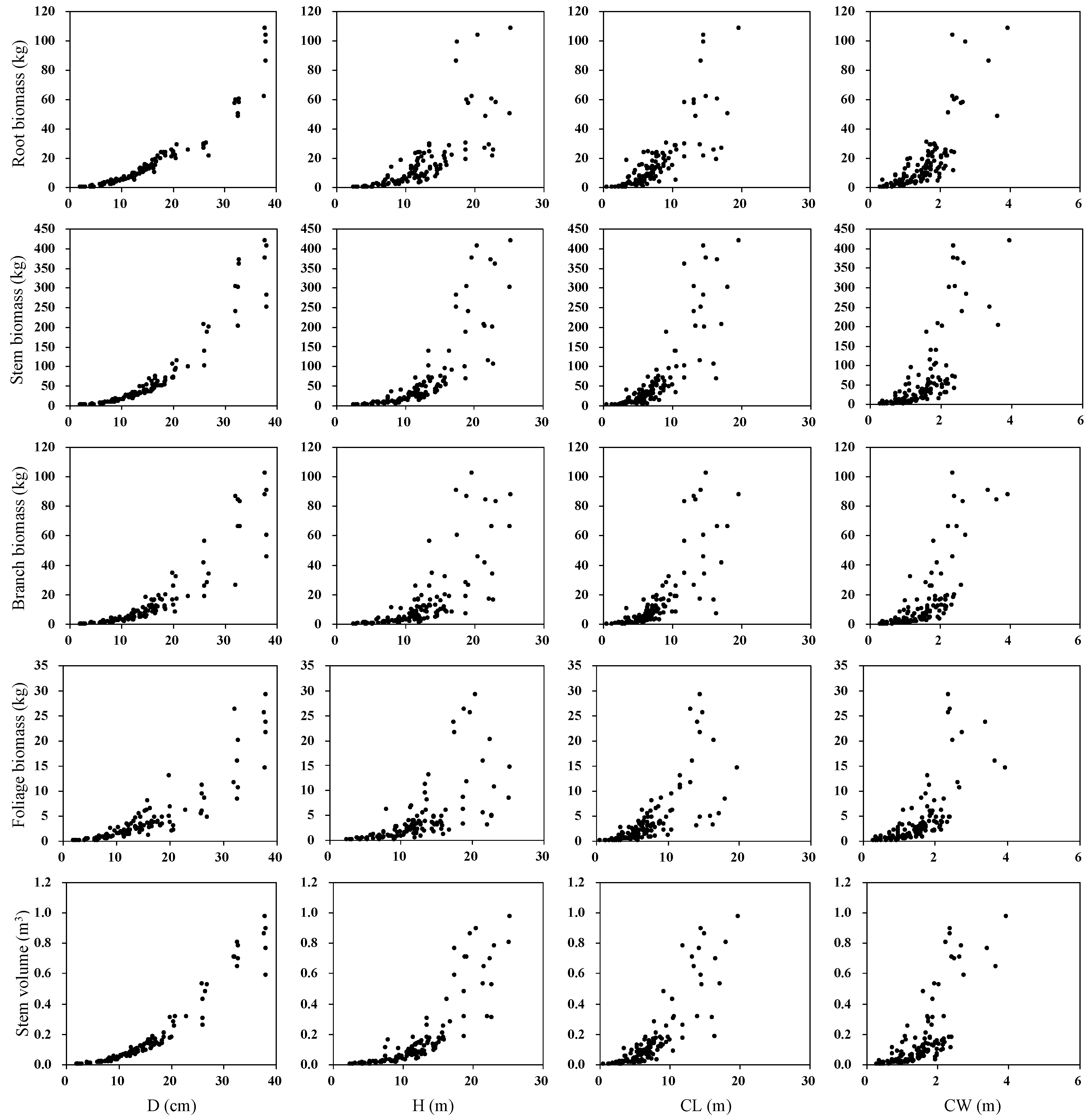
2.2.1. Tree Measurements

The selected sample trees in this study were required to meet several basic prerequisites: undamaged, healthy, with reasonably straight, single stems, and neither border trees nor dying trees. A total of 128 trees were collected using the destructive sampling method from artificial plantations spread across nine sites in HSP (Figure 1), where Populus × xiaohei is broadly distributed. The tree biomass and stem volume measurements were deliberately organized either in July or August. All of the sample trees were felled at the ground level point. The total tree height ($H$) and the length of the live crown ($CL$) of the selected sample trees were recorded directly after felling, while the measurement of crown width ($CW$) and diameter at breast height ($D$) had already been done in advance to tree felling. After the tree felling process was conducted successfully, the tree stem and live crown component were cut at the first live branch position. The characteristics of the sample trees in this study are listed in

Table 1. Summary statistics of tree variables, tree biomass, stem volume and biomass conversion and expansion factors for the sampled Populus × xiaohei trees.

Variables	N	Min	Max	Mean	SD
$D$ (cm)	128	2.0	38.0	14.3	8.5
$H$ (m)	128	2.5	25.3	11.8	5.0
$CL$ (m)	128	0.5	19.7	7.2	3.8
$CW \left(\mathrm{m}\right)$	128	0.3	4.0	1.5	0.7
$Age$ (year)	128	2.0	35.0	17.8	8.0
Total biomass (kg)	128	0.62	630.52	93.78	134.01
Root biomass (kg)	128	0.11	108.13	15.49	20.19
Stem biomass (kg)	128	0.34	420.27	60.74	90.42
Branch biomass (kg)	128	0.06	102.15	13.65	21.13
Foliage biomass (kg)	128	0.01	29.07	3.90	5.48
Stem volume (m3)	128	0.0009	0.9740	0.1555	0.2145

.

2.2.2. Biomass Measurements

For stem biomass measurements, the stems were partitioned into 1 m length approximate cylinders, and each of them was weighed using a dynamometer. Further, a 2–3 cm disc subsampled from the base and the top of each approximate cylinder was weighed and transmitted to the laboratory for analyzing the dry/fresh weight ratio (DFWR). For branch and foliage biomass measurements, the total fresh weight of all live tree branches (unseparated branches and foliage) within the canopy was weighed. The branch and foliage biomass were measured by sampling approximately 9–15 branches, which were equally distributed throughout the canopy. Then, the branch and foliage from each sample were separated, weighed, and subsampled for determining the DFWR. The tree roots were excavated by using both manual digging and lifting machines within the 3 m radius of the excavation zone. Due to the high difficulty level and time limitation, in this study, the fine roots (diameter < 5 mm) were intentionally left out. All roots were sorted into three different categories, i.e., small (diameter < 2 cm), medium (diameter 2–5 cm), and large (diameter > 5 cm), and weighed. The fresh weight from each root class was sampled and transmitted to the laboratory for determining the DFWR. The DFWR was then used to determine the dry weight value of each tree component by multiplying with its respective fresh weight. The total tree biomass was acquired by summing the stem, root, branch, and foliage dry weight. The descriptive statistics of all sampled trees used in this study are listed in Table 1. The relationships between the dependent (components biomass) and independent variables are presented in Figure 2.

2.2.3. Stem Volume and Biomass Conversion and Expansion Factor $\left(BCEF\right)$ Measurements

The stem volume (V) was calculated by aggregating each stem’s section volume, based on a 1 m length of stem cylinders’ volume and a treetop for each sampled tree. The Smallian’s formula [50] was used to compute the stem volumes:

$$V=\left[\frac{1}{2}\left(g_0+g_n\right)+{\sum }_{i=1}^{n-1}{g}_i\right]l+\frac{1}{3}{g}_n{l}^{\prime }$$

(1)

where $g_0$ is the basal area at the stem base (tree felling point); $g_n$ is the basal area at the topmost of the tree stem (excluding treetop); $g_i$ is the basal area at the upper side of each stem section; $l$ is the length of stem section, which is 1 m in this study; $l^{\prime }$is the length of the treetop;$n$ is the number of stem sections in each sampled tree. After the stem volume of each tree was obtained, we measured the $BCE{F}_s$ value of the four primary biomass components using the following equation:

$$BCE{F}_i=\frac{W_i}{V}$$

(2)

where $BCE{F}_i$ represents the biomass conversion factor for each component in kg/m³ (i = r for root, s for stem, b for branch, and f for foliage); $W_i$ represents the dry biomass of each respective component in kg; and $V$ is the volume of the stem component in m³.

2.2.4. Carbon Concentration Measurements

Carbon concentrations of root, stem, branch, and foliage were measured using oven-dried samples. Due to the time limitation and absence of samples, in this study, only 140 samples of stem, root, branch, and foliage from 35 trees were used to determine the carbon concentration of Populus × xiaohei. All samples were then burned entirely at a temperature of 1200 °C in a vial containing pure oxygen, and the emitted carbon in the form of CO₂ was measured with a non-dispersion infrared ray (NDIR) analyzer (Multi N/C 3000 analyzer with 1500 Solids Module, Analytik Jena AG, Germany). Hence, the carbon content (kg) of each tree component can be calculated by simply multiplying its biomass and carbon concentration.

2.3. Statistical Analysis

2.3.1. Variable Selection of Biomass and Volume Models

It is well-known that the power-law function is usually used to predict the biomass and volume of an individual tree. In this study, the relationships between the tree biomass components and several available predictors were screened through visual inspection to ascertain that the component biomass and volume models can be developed as a multivariate power-law function (Figure 2). Further, the power-law functions with an additive error term were determined to develop the biomass and volume models for Populus × xiaohei. The function form is as follows:

$$Y_i=e^{{\beta }_{i0}}{X}_1^{{\beta }_{i1}}{X}_2^{{\beta }_{i2}}\cdots X_k^{{\beta }_{ik}}+{\epsilon }_i$$

(3)

where $Y_i$ represents the tree components’ biomass in kilograms (i = r for root, s for stem, b for branch, and f for foliage) or stem volume in cubic meters; $X_k$ is several tree predictors (j = 1, …, k), i.e., $D$, $H$, $CW$, and $CL$; ${\beta }_{ik}$ are the equations’ coefficients to be predicted; ${\epsilon }_i$ is the model error term.

Eight power-law functions in

Table 2. Fit statistics of the eight biomass models based on several combinations of different predictors for each tree component of Populus × xiaohei.

Components	Equations	${\mathit{R}}^2$	RMSE	AIC
Root	$W_r=e^{{\beta }_{r0}}{D}^{{\beta }_{r1}}$	0.9361	5.0829	783.48
	$W_r=e^{{\beta }_{r0}}{D}^{{\beta }_{r1}}{H}^{{\beta }_{r2}}$	0.9369	5.0526	783.94
	$W_r=e^{{\beta }_{r0}}{D}^{{\beta }_{r1}}C{W}^{{\beta }_{r2}}$	0.9446	4.7349	767.32
	$W_r=e^{{\beta }_{r0}}{D}^{{\beta }_{r1}}C{L}^{{\beta }_{r2}}$	0.9360	5.0873	785.70
	$W_r=e^{{\beta }_{r0}}{D}^{{\beta }_{r1}}{H}^{{\beta }_{r2}}C{W}^{{\beta }_{r3}}$	0.9460	4.6723	765.91
	$W_r=e^{{\beta }_{r0}}{D}^{{\beta }_{r1}}{H}^{{\beta }_{r2}}C{L}^{{\beta }_{r3}}$	0.9369	5.0507	785.85
	$W_r=e^{{\beta }_{r0}}{D}^{{\beta }_{r1}}C{L}^{{\beta }_{r2}}C{W}^{{\beta }_{r3}}$	0.9446	4.7338	769.26
	$W_r=e^{{\beta }_{r0}}{D}^{{\beta }_{r1}}{H}^{{\beta }_{r2}}C{L}^{{\beta }_{r3}}C{W}^{{\beta }_{r4}}$	0.9463	4.6608	767.28
Stem	$W_s=e^{{\beta }_{s0}}{D}^{{\beta }_{s1}}$	0.9323	23.443	1174.82
	$W_s=e^{{\beta }_{s0}}{D}^{{\beta }_{s1}}{H}^{{\beta }_{s2}}$	0.9686	15.9484	1078.20
	$W_s=e^{{\beta }_{s0}}{D}^{{\beta }_{s1}}C{W}^{{\beta }_{s2}}$	0.9349	22.9881	1171.80
	$W_s=e^{{\beta }_{s0}}{D}^{{\beta }_{s1}}C{L}^{{\beta }_{s2}}$	0.9448	21.1674	1150.68
	$W_s=e^{{\beta }_{s0}}{D}^{{\beta }_{s1}}{H}^{{\beta }_{s2}}C{W}^{{\beta }_{s3}}$	0.9743	14.4471	1054.89
	$W_s=e^{{\beta }_{s0}}{D}^{{\beta }_{s1}}{H}^{{\beta }_{s2}}C{L}^{{\beta }_{s3}}$	0.9696	15.7087	1076.33
	$W_s=e^{{\beta }_{s0}}{D}^{{\beta }_{s1}}C{L}^{{\beta }_{s2}}C{W}^{{\beta }_{s3}}$	0.9482	20.4911	1144.37
	$W_s=e^{{\beta }_{s0}}{D}^{{\beta }_{s1}}{H}^{{\beta }_{s2}}C{L}^{{\beta }_{s3}}C{W}^{{\beta }_{s4}}$	0.9753	14.1656	1051.86
Branch	$W_b=e^{{\beta }_{b0}}{D}^{{\beta }_{b1}}$	0.8640	7.7596	891.78
	$W_b=e^{{\beta }_{b0}}{D}^{{\beta }_{b1}}{H}^{{\beta }_{b2}}$	0.8672	7.6678	890.73
	$W_b=e^{{\beta }_{b0}}{D}^{{\beta }_{b1}}C{W}^{{\beta }_{b2}}$	0.8711	7.5563	886.98
	$W_b=e^{{\beta }_{b0}}{D}^{{\beta }_{b1}}C{L}^{{\beta }_{b2}}$	0.8678	7.6515	890.18
	$W_b=e^{{\beta }_{b0}}{D}^{{\beta }_{b1}}{H}^{{\beta }_{b2}}C{W}^{{\beta }_{b3}}$	0.8732	7.4942	886.86
	$W_b=e^{{\beta }_{r0}}{D}^{{\beta }_{b1}}{H}^{{\beta }_{b2}}C{L}^{{\beta }_{b3}}$	0.8672	7.6674	892.71
	$W_b=e^{{\beta }_{b0}}{D}^{{\beta }_{b1}}C{L}^{{\beta }_{b2}}C{W}^{{\beta }_{b3}}$	0.8732	7.494	886.86
	$W_b=e^{{\beta }_{b0}}{D}^{{\beta }_{b1}}{H}^{{\beta }_{b2}}C{L}^{{\beta }_{b3}}C{W}^{{\beta }_{b4}}$	0.8725	7.5151	889.58
Foliage	$W_f=e^{{\beta }_{f0}}{D}^{{\beta }_{f1}}$	0.8346	2.2203	571.44
	$W_f=e^{{\beta }_{f0}}{D}^{{\beta }_{f1}}{H}^{{\beta }_{f2}}$	0.8629	2.0212	549.39
	$W_f=e^{{\beta }_{f0}}{D}^{{\beta }_{f1}}C{W}^{{\beta }_{f2}}$	0.8321	2.2369	575.35
	$W_f=e^{{\beta }_{f0}}{D}^{{\beta }_{f1}}C{L}^{{\beta }_{f2}}$	0.8407	2.1788	568.62
	$W_f=e^{{\beta }_{f0}}{D}^{{\beta }_{f1}}{H}^{{\beta }_{f2}}C{W}^{{\beta }_{f3}}$	0.8603	2.0406	553.84
	$W_f=e^{{\beta }_{f0}}{D}^{{\beta }_{f1}}{H}^{{\beta }_{f2}}C{L}^{{\beta }_{f3}}$	0.8629	2.0213	551.41
	$W_f=e^{{\beta }_{f0}}{D}^{{\beta }_{f1}}C{L}^{{\beta }_{f2}}C{W}^{{\beta }_{f3}}$	0.8385	2.1941	572.41
	$W_f=e^{{\beta }_{f0}}{D}^{{\beta }_{f1}}{H}^{{\beta }_{f2}}C{L}^{{\beta }_{f3}}C{W}^{{\beta }_{f4}}$	0.8598	2.0441	556.27

are used to estimate the tree components’ biomass and stem volume based on one predictor ($D$), two predictors ($D$ + $H$/$CL$/$CW$), three predictors ($D$ + $H$ + $CL$/$CW$), and four predictors ($D$ + $H$ + $CL$ + $CW$). All of the equations were tested to select the “best model” for each component biomass and stem volume equation by relying on the three indicators, i.e., Akaike information criterion ($AIC$), root mean squared error ($\mathrm{RMSE}$), and coefficient of determination ($R^2$). The models with the bigger $R^2$ and smaller $\mathrm{RMSE}$ and $AIC$ have better fitting performance. If the difference of the AIC between the two models is too small, there is no real distinction between them. Finally, the combinations of one, two, and the best predictors are determined as the primary structures for developing the three additive biomass model systems and the stem volume equation.

2.3.2. Additive Biomass Model System

Referring to the additive model configuration proposed by Affleck and Diéguez-Aranda [51], the additive system of four functions without applying any parameter restriction on the structural parameters can be written as follows:

$$\{\begin{array}{c}{W}_r=e^{{\beta }_{r0}}{X}_1^{{\beta }_{r1}}{X}_2^{{\beta }_{r2}}\cdots X_k^{{\beta }_{rk}}+{\epsilon }_r\\ W_s=e^{{\beta }_{s0}}{X}_1^{{\beta }_{s1}}{X}_2^{{\beta }_{s2}}\cdots X_k^{{\beta }_{sk}}+{\epsilon }_s \\ W_b=e^{{\beta }_{b0}}{X}_1^{{\beta }_{b1}}{X}_2^{{\beta }_{b2}}\cdots X_k^{{\beta }_{bk}}+{\epsilon }_b\\ W_f=e^{{\beta }_{f0}}{X}_1^{{\beta }_{f1}}{X}_2^{{\beta }_{f2}}\cdots X_k^{{\beta }_{fk}}+{\epsilon }_f\end{array}$$

(4)

where r, s, b and f represent roots, stems, branches, and foliage, respectively. The other abbreviations were the same as it written in Equation (2).

2.3.3. Weighting Function for Heteroscedasticity

The residuals of tree biomass and volume equations often increase with the increasing tree sizes’ ($D$), which is commonly known as heteroscedasticity. In terms of nonlinear regression, each biomass equation should have its own specialized weighting function to neutralize the heteroscedasticity problem effectively. Generally, a functional correlation occurred between the model’s independent variables and the model residuals of the ith observation. Thus, the equation of $var({\epsilon }_i)={\sigma }^2{\widehat{Y}}_i^{2\varphi }$ was specified to model the power variance function for further application in the tree biomass and stem volume equations, where ${\epsilon }_i$ represents the unweighted model residual, $\varphi$ is a coefficient to be predicted, ${\widehat{Y}}_i$ is the predicted biomass of each component and stem volume for the ith sample tree, and ${\sigma }^2$ is a scaling factor for the error dispersion.

2.3.4. Model Fitting and Evaluation

The model parameters in the stem volumes were estimated by utilizing the nonlinear ordinary least squares (OLS) as the fundamental method, while the additive biomass model system (ABMS) employed the nonlinear seemingly unrelated regression (NSUR) to estimate the coefficients. Further information about the algorithm and theory of NSUR may be found in each of the previously mentioned publications [22,52]. All the above model fittings were carried out using different available procedures in SAS 9.3 software such as PROC NLIN and PROC MODEL [53].

Further, the three ABMS and stem volume models’ performance based on different combinations of predictors were evaluated and compared using both statistical and graphical analyses. Two statistical indicators obtained from the model residuals and predicted values were used to assess and compare the performance of the model fitting: the coefficient of determination ($R^2$) and root mean square error (RMSE). Moreover, three statistical indicators of the leave-one-out method were utilized to evaluate the prediction performance: the mean prediction error percent (MPE), mean absolute percent error (MAPE), and model efficiency (EF) (similar to the coefficient of determination). The mathematical expressions are as follows:

$$R^2=1-\frac{{\sum }_{i=1}^n{(Y_i-{\widehat{Y}}_i)}^2}{{\sum }_{i=1}^n{(Y_i-\overline{Y})}^2}$$

(5)

$$\mathrm{RMSE}=\sqrt{\frac{{\sum }_{i=1}^n{\left(Y_i-{\widehat{Y}}_i\right)}^2}{n}}$$

(6)

$$\mathrm{MPE}=\frac{{\sum }_{i=1}^n\left(\left(Y_i-{\widehat{Y}}_{i,-i}\right)/\overline{Y}\right)}{n}\times 100$$

(7)

$$\mathrm{MAPE}=\frac{{\sum }_{i=1}^n\left|(Y_i-{\widehat{Y}}_{i,-i})/Y_i\right|}{n}\times 100$$

(8)

$$EF=1-\frac{{\sum }_{i=1}^n{(Y_i-{\widehat{Y}}_{i,-i})}^2}{{\sum }_{i=1}^n{(Y_i-\overline{Y})}^2}$$

(9)

where $Y_i$ is the observed component biomass or stem volume value, ${\widehat{Y}}_i$ is the estimated biomass or stem volume of the model, which were fitted by using all of the sample trees ($n$), $\overline{Y}$ is the mean value of the observed biomass or stem volume, ${\widehat{Y}}_{i,-i}$ is the predicted value of the leave-one-out method, which was estimated by using the leave-one-out observation model ($n-$1); $n$ was the total number of sampled trees.

In this study, the predictive performance of a biomass model was compared with previously published models for the particular tree species developed by Fan et al. [43] and Song et al. [44], and a stem volume model was compared with the published model developed by Yang et al. [49].

2.3.5. Effects of Tree Sizes (D) and Components on Carbon Concentration

To investigate the effect of the tree components on the variation of the carbon concentration, analysis of variance (ANOVA) with Tukey mean comparison was performed to examine the difference of the tree components’ carbon concentrations using PROC GLM procedure in SAS 9.3 software [53].

3. Results

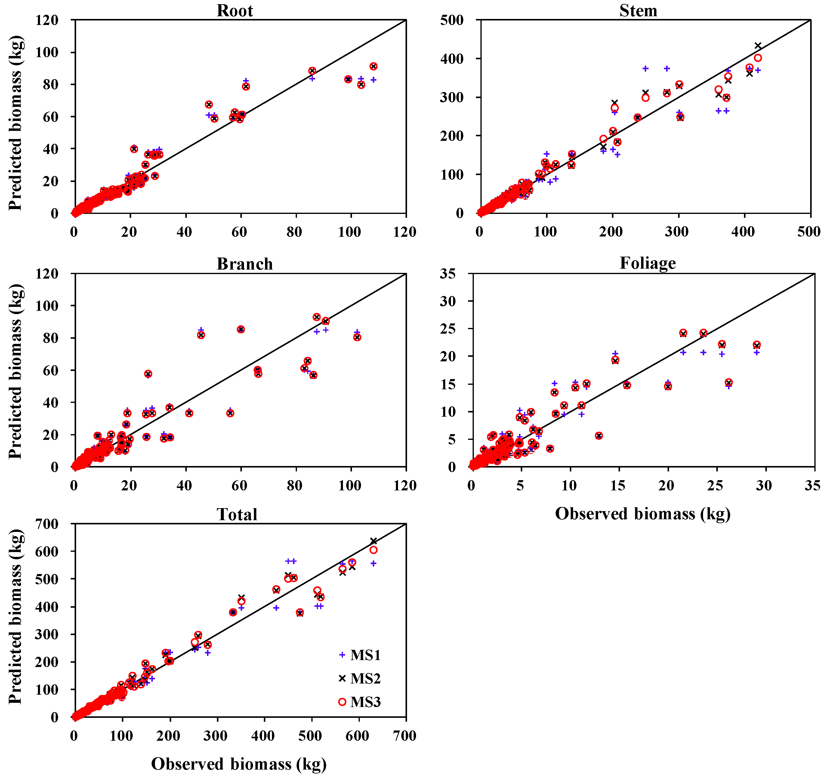
3.1. Biomass Equations

$D$ and $H$ are the most reliable predictors to develop a power-law allometric equation in the vast majority of the tree components and total biomass estimations. However, depending on the availability of the tree biomass data and research goals, $CL$and $CW$ may become potential predictors to improve the model fitting performance of biomass models. In the present research, the four predictors ($D$, $H$, $CW$, and$CL$) were separately fitted to each component biomass equation.

Table 3. Parameter estimates, standard errors (in parenthesis), goodness-of-fit statistics, jackknifing validations, and the parameter of weight functions (ϕ) for three additive biomass model systems based on different predictor variables.

Model Systems	Components	βi0	βi1	βi2	βi3	βi4	R2	RMSE	ϕ	MPE	MAPE	EF
MS1	Root	−3.0963 ** (0.1163)	2.0676 ** (0.0378)				0.9363	5.0361	0.5500	0.38	29.04	0.9283
	Stem	−2.7171 ** (0.1324)	2.3758 ** (0.0418)				0.9316	23.3782	0.5040	2.35	18.28	0.9209
	Branch	−4.1284 ** (0.2534)	2.3560 ** (0.0768)				0.8640	7.6981	0.3500	0.46	37.51	0.8434
	Foliage	−4.4739 ** (0.2364)	2.0621 ** (0.0773)				0.8321	2.2194	0.5650	2.07	53.17	0.8168
	Total	—	—				0.9633	25.5756		1.74	13.86	0.9578
MS2	Root	−2.7455 ** (0.1447)	1.8924 ** (0.0599)	0.2784 ** (0.0775)			0.9442	4.6942	0.5356	−0.01	27.96	0.9324
	Stem	−3.6308 ** (0.1238)	1.8585 ** (0.0537)	0.9137 ** (0.0779)			0.9685	15.8047	0.4968	−0.02	14.25	0.9627
	Branch	−3.8488 ** (0.3012)	2.2030 ** (0.1144)	0.2750 * (0.1361)			0.8702	7.4923	0.3375	0.52	35.46	0.8419
	Foliage	−4.0767 ** (0.2724)	2.4441 ** (0.1387)	−0.5718 * (0.1894)			0.8578	2.0182	0.5503	1.42	53.92	0.8459
	Total	—	—	—			0.9781	19.7545		0.12	10.08	0.9748
MS3	Root	−2.7445 ** (0.1447)	1.8919 ** (0.0599)	0.2794 ** (0.0775)			0.9442	4.6938	0.5356	−0.02	27.95	0.9321
	Stem	−4.0585 ** (0.1600)	2.0416 ** (0.0700)	1.0536 ** (0.0955)	−0.1871 ** (0.0557)	−0.1709 * (0.0733)	0.9741	14.2158	0.4965	0.04	12.60	0.9664
	Branch	−3.8541 ** (0.3011)	2.2050 ** (0.1144)	0.2745 * (0.1359)			0.8701	7.4940	0.3375	0.46	35.43	0.8413
	Foliage	−4.0972 ** (0.2722)	2.4532 ** (0.1383)	−0.5734 * (0.1888)			0.8603	2.0165	0.5503	1.09	53.68	0.8459
	Total	—	—	—	—	—	0.9800	18.8546		0.14	11.10	0.9755

**: Statistically significant parameters at the significance level p < 0.001; *: Statistically significant parameters at the significance level p < 0.05; ns: non-significant (p > 0.05).

displays the result statistics of the model fitting, including $R^2$, $RMSE$, and $AIC$. $H$, $CW$, and $CL$ were found to give a significant improvement as the predictors for the stem biomass equation. The integration of $CW$ into the root and branch biomass models gave a significant enhancement into the model fitting quality. Meanwhile, both $H$ and $CL$ were found to be insignificant for the branch and root biomass equations since they yielded a similar $R^2$, $RMSE$, and AIC compared to the biomass model developed with the combination of $D$and $CW$. Thus, they were excluded from the root equation. Similarly, $CW$ and $CL$ were also excluded for foliage biomass equations. Hence, several predictors were determined as the best variable combinations to develop the power-law function for each component biomass equations: $D$ and $CW$ were selected for root and branch biomass equations; $D$, $H$, $CL$, and $CW$ were chosen for stem biomass equations; $D$ and $H$ were preferred for foliage biomass equations. Furthermore, we fitted the three additive biomass model systems based on D as the sole predictor (namely MS1, Equation (10)), $D$ and $H$ or $CW$ as two predictors (namely MS2, Equation (11)), and best predictors (namely MS3, Equation (12)).

$$\{\begin{array}{c}{W}_r=e^{{\beta }_{r0}}{D}^{{\beta }_{r1}}+{\epsilon }_r \\ W_s=e^{{\beta }_{s0}}{D}^{{\beta }_{s1}}+{\epsilon }_s \\ W_b=e^{{\beta }_{b0}}{D}^{{\beta }_{b1}}+{\epsilon }_b\\ W_f=e^{{\beta }_{f0}}{D}^{{\beta }_{f1}}+{\epsilon }_f\end{array}$$

(10)

$$\{\begin{array}{c}{W}_r=e^{{\beta }_{r0}}{D}^{{\beta }_{r1}}C{W}^{{\beta }_{r2}}+{\epsilon }_r\\ W_s=e^{{\beta }_{s0}}{D}^{{\beta }_{s1}}{H}^{{\beta }_{s2}}+{\epsilon }_s \\ W_b=e^{{\beta }_{b0}}{D}^{{\beta }_{b1}}C{W}^{{\beta }_{b2}}+{\epsilon }_b\\ W_f=e^{{\beta }_{f0}}{D}^{{\beta }_{f1}}{H}^{{\beta }_{f2}}+{\epsilon }_f \end{array}$$

(11)

$$\{\begin{array}{c}{W}_r=e^{{\beta }_{r0}}{D}^{{\beta }_{r1}}C{W}^{{\beta }_{r2}}+{\epsilon }_r\\ W_s=e^{{\beta }_{s0}}{D}^{{\beta }_{s1}}{H}^{{\beta }_{s2}}C{L}^{{\beta }_{s3}}C{W}^{{\beta }_{s4}}+{\epsilon }_s\\ W_b=e^{{\beta }_{b0}}{D}^{{\beta }_{b1}}{H}^{{\beta }_{b2}}C{W}^{{\beta }_{b3}}+{\epsilon }_b \\ W_f=e^{{\beta }_{f0}}{D}^{{\beta }_{f1}}{H}^{{\beta }_{f2}}+{\epsilon }_f\end{array}$$

(12)

The coefficient estimates, standard errors (SEs), and goodness of fit of the three additive biomass equation systems based on several different predictors are presented in

Table 4. Parameter estimates, standard errors (in parenthesis), goodness-of-fit statistics, jackknifing validations, and the parameter of weight functions (ϕ) for eight stem volume equations based on different predictor variables for Populus × xiaohei trees.

Equations	β0	β1	β2	β3	β4	R2	RMSE	AIC	ϕ	MPE	MAPE	EF
$V=e^{{\beta }_0}{D}^{{\beta }_1}$	−8.1001 ** (0.1434)	2.1995 ** (0.0432)				0.9498	0.0479	−410.70	0.6010	−0.63	26.7245	0.9416
$V=e^{{\beta }_0}{D}^{{\beta }_1}{H}^{{\beta }_2}$	−9.1235 ** (0.1155)	1.7252 ** (0.0432)	0.8949 ** (0.0629)			0.9845	0.0266	−559.46	0.6441	−0.26	14.9243	0.9807
$V=e^{{\beta }_0}{D}^{{\beta }_1}C{L}^{{\beta }_2}$	−8.0681 ** (0.1267)	1.8657 ** (0.0724)	0.4289 ** (0.0782)			0.9605	0.0425	−439.56	0.6575	−0.35	24.9401	0.9526
$V=e^{{\beta }_0}{D}^{{\beta }_1}C{W}^{{\beta }_2}$	−8.2324 ** (0.1781)	2.2634 ** (0.0678)	−0.0955 ns (0.0806)			0.9498	0.0479	−408.73	0.6214	−0.49	26.9817	0.9390
$V=e^{{\beta }_0}{D}^{{\beta }_1}{H}^{{\beta }_2}C{L}^{{\beta }_3}$	−9.2455 ** (0.1341)	1.7788 ** (0.0514)	0.9813 ** (0.0838)	−0.1222 ns (0.0699)		0.9853	0.0259	−564.04	0.7114	−0.18	14.3864	0.9813
$V=e^{{\beta }_0}{D}^{{\beta }_1}{H}^{{\beta }_2}C{W}^{{\beta }_3}$	−9.3333 ** (0.1314)	1.8184 ** (0.0516)	0.9024 ** (0.0606)	−0.1489 ** (0.0486)		0.9860	0.0253	−570.38	0.6508	−0.23	15.3972	0.9823
$V=e^{{\beta }_0}{D}^{{\beta }_1}C{L}^{{\beta }_2}C{W}^{{\beta }_3}$	−8.2102 ** (0.1577)	1.9390 ** (0.0862)	0.4209 ** (0.0774)	−0.0966 ns (0.0718)		0.9609	0.0423	−438.72	0.6926	−0.24	25.1799	0.9523
$V=e^{{\beta }_0}{D}^{{\beta }_1}{H}^{{\beta }_2}C{L}^{{\beta }_3}C{W}^{{\beta }_4}$	−9.4847 ** (0.1487)	1.8789 ** (0.0582)	1.0105 ** (0.0797)	−0.1409 * (0.0663)	−0.1564 ** (0.0485)	0.9869	0.0245	−576.36	0.6633	−0.29	14.9778	0.9826

**: Statistically significant parameters at the significance level p < 0.001; *: Statistically significant parameters at the significance level p < 0.05; ns: non-significant (p > 0.05).

. The results suggested that all of the estimated parameters in the three additive biomass model systems were statistically significant at the significance level p < 0.05; The $R^2$ values for all component biomass equations in MS1 are 0.9363, 0.9316, 0.8640, and 0.8321 for the root, stem, branch, and foliage, respectively. Then, all of the component biomass equations were summed, and the $R^2$ value for the total biomass estimation was calculated, which was 0.9633. Compared to the MS1, MS2 owned a smaller $RMSE$ and greater $R^2$ for total and component biomass equations. An apparent increase in the $R^2$ value along with a notable decrease in $RMSE$ was shown for stem and foliage biomass models, which were approximately 4.0% and 3.1% for $R^2$, respectively, and about 32.4% and 9.1% for $RMSE$, respectively. A slight increase in $R^2$ and decrease in $RMSE$ were exhibited for the branch and root biomass models, which was around 0.8% and 0.7% for $R^2$, respectively, and about 6.8% and 2.8% for $RMSE$, respectively. The model fitting result based on the best combination of predictors, MS3, yielded a lower error estimation than MS1 and MS2, especially for the stem biomass model, which was indicated by having a more than 10% decrease in $RMSE$ compared to the $D$-only equation.

Figure 3 presents the scatter diagram between the observed and predicted biomass results for the three additive biomass models’ total and components biomass. Figure 3 also indicated that both MS2 and MS3 yielded higher fitting performance than MS1. Overall, adding $H$ or $CW$ could improve the accuracy of the root, stem, branch, and foliage biomass estimations. The poorest model fittings were obtained in branch and foliage biomass models with relatively larger $RMSE$ and lower $R^2$, while the best fittings were found in the root, stem, and total biomass models.

Moreover, three constants of the 4 × 4 matrices were expected for cross-correlations of residuals amongst all four components’ equations for MS1, MS2, and MS3. Apparently, specific correlations existed between the root and branch biomass models, between the foliage and branch biomass equations across the entire model systems (MS1, MS2, and MS3), and between the stem and foliage biomass models in MS2 and MS3, as shown in the following three correlation matrices:

$$\begin{array}{cc}MS\mathbf{1}& \begin{array}{cccc}\hspace{1em} \mathrm{Root}& \hspace{1em}\mathrm{Stem}& \hspace{1em}\mathrm{Branch} & \mathrm{Foliage}\end{array}\\ \begin{array}{c}\mathrm{Root}\\ \mathrm{Stem}\\ \mathrm{Branch}\\ \mathrm{Foliage}\end{array}& \left(\begin{array}{cccc}1.0000& -0.0684& -0.2540& 0.0273\\ -0.0684& 1.0000& 0.0735& 0.0285\\ -0.2540& 0.0735& 1.0000& 0.3296\\ 0.0273& 0.0285& 0.3296& 1.0000\end{array}\right)\end{array}$$

$$\begin{array}{cc}MS\mathbf{2}& \begin{array}{cccc}\hspace{1em} \mathrm{Root}& \hspace{1em}\mathrm{Stem}& \hspace{1em}\mathrm{Branch} & \mathrm{Foliage}\end{array}\\ \begin{array}{c}\mathrm{Root}\\ \mathrm{Stem}\\ \mathrm{Branch}\\ \mathrm{Foliage}\end{array}& \left(\begin{array}{cccc}1.0000& -0.0169& -0.3285& -0.0354\\ -0.0169& 1.0000& 0.1016& 0.3403\\ -0.3285& -0.3315& 1.0000& 0.3308\\ -0.0354& 0.3403& 0.3308& 1.0000\end{array}\right)\end{array}$$

$$\begin{array}{cc}MS\mathbf{3}& \begin{array}{cccc}\hspace{1em} \mathrm{Root}& \hspace{1em}\mathrm{Stem}& \hspace{1em}\mathrm{Branch} & \mathrm{Foliage}\end{array}\\ \begin{array}{c}\mathrm{Root}\\ \mathrm{Stem}\\ \mathrm{Branch}\\ \mathrm{Foliage}\end{array}& \left(\begin{array}{cccc}1.0000& -0.0055& -0.3284& -0.0356\\ -0.0055& 1.0000& 0.1367& 0.4308\\ -0.3284& 0.1367& 1.0000& 0.3308\\ -0.0356& 0.4308& 0.3308& 1.0000\end{array}\right)\end{array}$$

The model validations (i.e., MPE, MAPE, and EF) of the three additive biomass model systems are presented in Table 3. The results showed that the MPE values were relatively close to 0 for the entire three model systems. For the stem and total biomass, a relatively small prediction error (MAPE% < 20%) was found within the three additive systems. MS2 and MS3 yielded smaller MPE and MAPE and larger $EF$ than MS1, but there was no discernible difference between MS2 and MS3. Contrarily, the biomass models for the other three components gave less precise predictions, especially for foliage components, than those for the stem and total biomass.

Furthermore, Figure 4 presents the biomass partitioning formed by using biomass models developed in this study for each primary component, such as root, stem, branch, and foliage. It showed that the trend was inconsistent between each component. Stem biomass relative contribution to total biomass increased as $D$ increased, while root biomass relative contribution decreased as $D$ increased. Nevertheless, branch and foliage biomass had slight alterations with $D$ increased. Overall, the average biomass proportion was approximately 19.7% for the root, 61.2% for the stem, 14.2% for the branch, and 4.9% for the foliage.

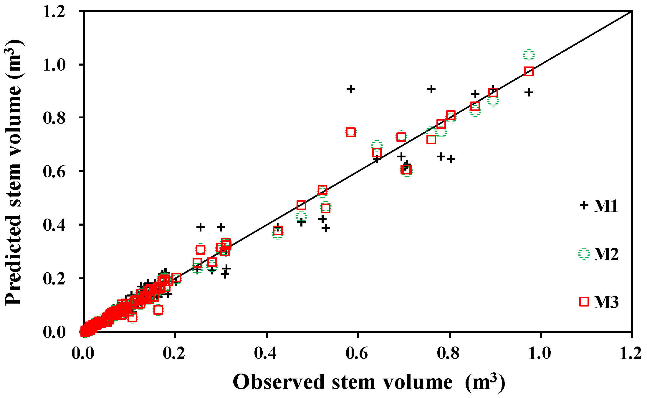
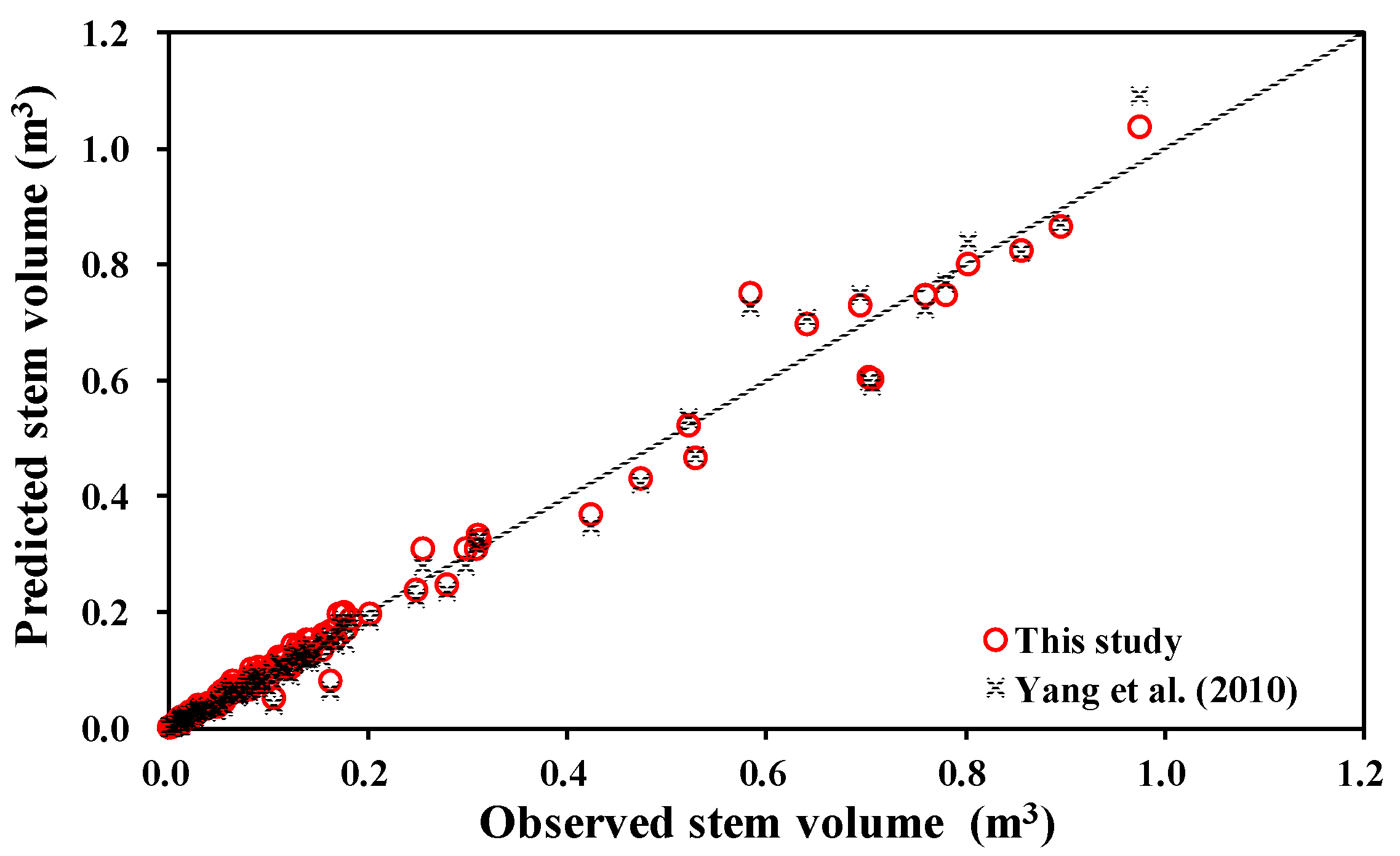
3.2. Stem Volume Equations

Similar to the biomass models above, eight power-law functions based on different combinations of predictors are also presented to estimate the stem volume. The best model was determined by R², $RMSE$, and $AIC$. As expected, D presents a strong relationship with stem volume ($R^2=0.95$), and adding $H$ into the model can significantly improve the model reliability ($R^2=0.98$). The combination of $CW$ and $CL$ slightly improved the fitting performance. In addition, MPE, MAPE, and EF were used to validate the prediction performance. The results showed that the MPE were close to 0, and the magnitudes of prediction errors were relatively small (MAPE < 30%) for all models. Two stem volume equations with different combinations of predictors ($D+H$) and ($D+H+CL+CW$) have better prediction performance compared to the other six equations (Table 4 and Figure 5).

It is worth recalling that the tree biomass could be estimated by multiplying the stem volume estimates by $BCE{F}_s$. Unfortunately, we were unsuccessful in attempting to develop the biomass conversion factor models. The main reasons behind this nonfulfillment are (1) there were no significant correlations detected between the $BCE{F}_s$ of each of the biomass components and tree variables; and (2) each biomass component had a linear relationship with the stem volume, especially for the stem component itself. In this study, $BCE{F}_s$ of different components at the tree level were calculated in order to provide a constant value for each component of the tree, which were 118.2 kg/m³ for the root, 380.2 kg/m³ for the stem, 90.7 kg/m³ for the branch, and 31.2 kg/m³ for the foliage (

Table 5. Constant (average value) of $BCE{F}_s$ calculated for Populus × xiaohei trees (kg/m³).

Components	N	Min	Max	Mean	SD
Root	128	28.8	296.7	118.2	41.1
Stem	128	199.1	616.0	380.2	67.3
Branch	128	28.9	266.7	90.7	44.6
Foliage	128	4.7	89.1	31.2	16.9

). The $BCE{F}_s$ results from this study may be used as a constant to estimate biomass or carbon stock for Populus × xiaohei since the values indicated were already stabilized; henceforth, the biomass or carbon stock estimation errors may be minimized.

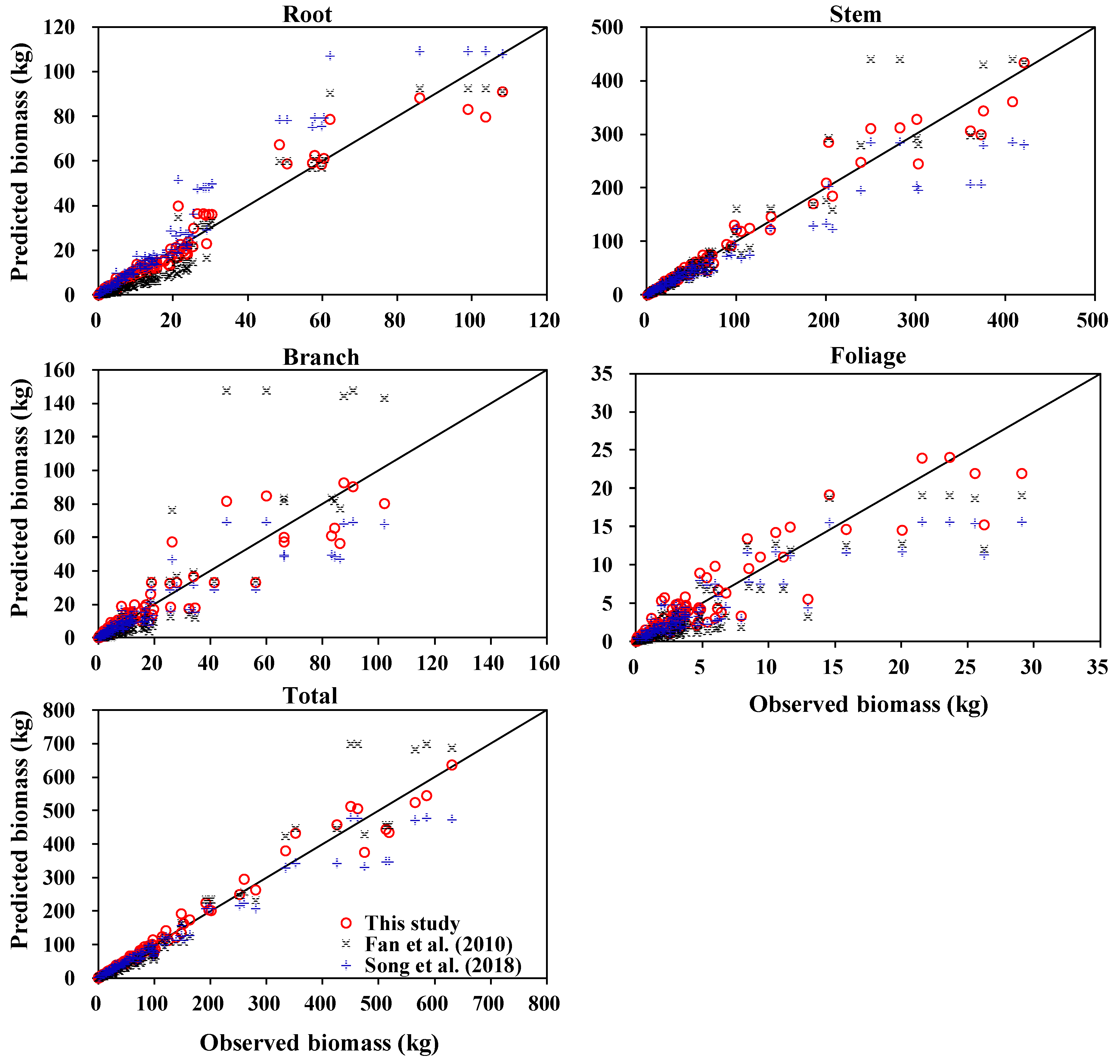
3.3. Comparison with Other Biomass and Stem Volume Models

The new biomass model system based on $D$-only (MS1) developed in this study was compared with the previously developed biomass models based on $D$-only from Fan et al. [41] and Song et al. [42]. The relationship between the predicted and observed value was scrutinized for each component and total biomass (Figure 6). The results showed that the new biomass model system predicted all biomass components better than the previous models, which was evaluated by the mean absolute prediction error (MAPE) and the coefficient of determination (R²). Specifically, Fan et al.’s models may have serious errors in the total, root, stem, and branch biomass estimations, in which the MAPE was 30.9%, 49.0%, 20.6%, and 64.3% for total, root, and foliage, respectively, while Song et al.’s models had a relatively large error in the total, root, and stem biomass estimations, in which the MAPE was 15.6%, 37.0%, and 20.2% for the total, root, and stem, respectively (Figure 6). Meanwhile, the MAPE values of our newly developed biomass equations (MS1) were consistently smaller than both of these two previous equations throughout all categories: 29.0% for the root, 18.3% for the stem, 37.5% for the branch, 53% for the foliage, and 14% for the total biomass equation (Table 3). Furthermore, a relatively similar pattern was also shown for the R². This study consistently delivered the highest R² values for the root, stem, branch, foliage, and total biomass equations, as much as 0.94, 0.93, 0.86, 0.83, and 0.96, respectively (Table 3). The equations developed by Fan et al., [41] gave the lowest R² values for both branch (0.41) and total biomass (0.91), while Song et al.’s [42] models gave the lowest R² for the root (0.82), stem (0.86), and foliage (0.75) biomass components.

We also compared the newly developed stem volume model based on $D$ and $H$ with the previously developed stem volume model based on $D$ and $H$ from Yang et al. [50] (Figure 7). The results showed that Yang et al.’s model produced similar predictions in estimating the stem volume, in which the MAPE is 1.5% smaller compared to the model developed in this study (Figure 7). However, the R² of the stem volume model of this study (0.9845) is slightly higher than Yang et al.’s (0.9807).

3.4. Variations of Carbon Concentration

Each component had different carbon concentrations; thus, acquiring the tree components’ carbon concentrations is of great importance to estimate the carbon stock accurately. After each component’s carbon stock value was acquired, they were summed to yield the total carbon stock value. The summary statistics of the carbon concentration values for each component and mean carbon concentration values by weighting biomass (WMCC) are given in

Table 6. Carbon concentration (%) by components along with the weighted mean carbon concentration (WMCC) statistics for Populus × xiaohei trees.

Components	Min	Max	Mean	SD
Root	42.31	50.00	45.98a	2.31
Stem	41.88	50.65	47.74b	1.84
Branch	43.29	51.61	48.32b	1.95
Foliage	45.56	52.18	48.46b	1.90
WMCC	44.38	49.64	47.43	1.51

. The tree components were confirmed to significantly affect the carbon concentration (at the 5% threshold, F value = 15.92, and p < 0.001). The foliage had the largest carbon concentration among the tree components, while the root had the lowest carbon concentration. The multiple comparisons based on Tukey mean comparison indicated that there is a clear distinction between root and stem, branch, and foliage carbon concentrations, while there is no real distinction between the stem, branch, and foliage carbon concentrations.

4. Discussion

Biomass additivity is an essential property of biomass equations that generally need to be considered to predict the components and total biomass estimations accurately. However, countless biomass equations found in the literature did not consider the additivity property and were separately developed to predict the total and components biomass [54,55]. There are many available procedures to achieve the additivity property of nonlinear biomass models; the most successful ones are those including contemporaneous correlations to force additivity, which is widely known as nonlinear seemingly unrelated regression (NSUR) [22,38]. In general, NSUR parameter estimates are always at least as efficient as nonlinear ordinary least square (OLS) for large sample sizes. However, in small sample sizes, the need to estimate the covariance matrix from the OLS residuals increases the sampling variability of the SUR estimates, or when there is no contemporaneous correlation of errors across equations, NSUR parameter estimates are the same or less efficient than those produced by OLS [41,53,56]. In addition, if the same or different predictors are considered in nonlinear biomass models, the heteroscedasticity needs to be corrected by different weights for each component biomass equation [22,38,56]. At this juncture, NSUR is found to be the most appropriate parameter estimation method. In the present study, we used one, two, and the best predictors as the primary structures to construct the three additive biomass model systems for Populus × xiaohei, in which each equation has a different weighting function. Furthermore, the cross-correlations matrix of residuals among all four equations showed that certain correlations existed between biomass components measured on the same individuals. These findings suggest that NSUR would result in a more efficient estimation than OLS. To date, several model specifications have been proposed for forcing the additivity of nonlinear equations [39,52]. The additive model structure proposed by Parresol [41] has become a standard for developing biomass equations, in which the total biomass model was set up as the sum of the component models. Many studies found that the additive model structure without the total biomass model, as proposed by Affleck and Diéguez-Aranda [51], was better to predict the total and components biomass than the initial Parresol’s model system [39,52,57]. Thus, the total biomass model was not present as a constraint in the additive model systems developed in the present study. In simple terms, the model systems of this study only fitted the four component biomass models.

Biomass models based on $D$ developed in the current study showed an excellent predictive ability for the total and components biomass, which explains 83% to 96% variations on the foliage and total biomass, respectively. Thus, $D$ is considered an irreplaceable independent variable in biomass modeling and usually acts as one of the most elementary measurement factors in forest inventory, which has been significantly recognized by other studies for various tree species [24,31,35]. For a given $D$, there is usually some variation among biomass components. In that case, $H$ and crown attributes ($CW$ and $CL$) were added to the models to enhance the biomass components models’ predictive ability. The additive biomass model systems with additional predictors ($H,$ $CW$, or $CL$) have generated a significant improvement in the model fitting and prediction performance. This finding is in accordance with those reported in the literature [38,40]. In addition, biomass equations with the involvement of some supportive predictors such as $H$, $CW$, and $CL$ are advantageous to increase the biomass predictions accuracy in response to the alterations in stand conditions (i.e., thinning) and is widely appropriate to be used in many ecological and forest management studies [38]. However, $H$, $CW,$ and $CL$ are generally difficult to obtain in practice, and also unfeasible to be implemented in China’s forest inventory. Thus, in most cases, only MS1 (based on $D$ equation system) can be used to provide accurate biomass predictions. To utilize MS2 and MS3 in estimating the total and components biomass, we need to measure the values of $H$, $CW$, and $CL$, or develop some models to firstly estimate $H,$ $CW$, and $CL$ from easily measurable predictors such as $D$ in future work.

To date, few biomass equations are available in the literature for Populus × xiaohei. The new biomass model based on $D$-only was compared with the previous biomass models developed by Fan et al. [43] and Song et al. [44]. The additive biomass model systems in this study were developed using a dataset from a wide geographical area; thus, they may be used in relatively wide coverage. Meanwhile, Fan et al. [43] used 18 Populus × xiaohei trees, of which the information about the range of $D$ is not given, and Song et al. [44] used 36 Populus × xiaohei trees, of which the range of $D$ is from 4.4 cm to 20 cm. Generally, the larger the sample size can reduce the parameter estimation’s uncertainty. Moreover, the biomass models developed by Fan et al. [43] lacked an additivity property and ignored the cross-correlations of residuals among all biomass equations. Compared to the two previous studies, both MAPE and R² obtained from the biomass models developed in this study (MS1) were found to be lower and higher across all components’ and total equations, respectively, indicating that the biomass models in the present study provide more accurate predictions than those developed by Fan et al. [43] and Song et al. [44], as simulated in Figure 6. The possible reasons are that the three studies’ data came from different sampling sites, and differences in the sample number, sample size ranges, and biomass measurement methods. These reasons could also lead to differences in soil conditions and growth processes [58].

In this study, power-law functions were used to develop the stem volume model for Populus × xiaohei trees. As used for our biomass models, $D$was also preferred as the main predictor since it has the ability to explain 95% of the stem volume variation. In addition, measuring $D$ is easier in practice and needs lower cost than other tree variables (i.e., $H$, $CW$, and $CL$). However, to improve the model precision, the combination of $D$ with other tree variables, e.g., $H$, $CW$, and $CL$, are proven to increase the precision of stem volume equations. Hence, we decided to consider three stem volume models based on $D$, $D+H$, and $D+H+CL+CW$ since these could be applied to the prediction of the stem volume. Compared with the previous stem volume equations developed by Yang et al. [50], both the new and the previous stem volume models provide almost the same prediction accuracy, as is expected. The potential explanation may be that the stem volume measurement method is uniform across different studies, in which only the dimeters at the base and the top of each stem section were measured.

Generally, biomass equations and $BCE{F}_s$ are categorized as one of the most important methods to estimate the biomass of an individual tree [23,59]. Tree stem volume is the only observed value required to estimate the tree biomass by utilizing the constant $BCE{F}_s$. However, many studies show that using the constant $BCE{F}_s$ values may induce serious errors in biomass estimation, and only provide satisfactory results in relation to stem biomass because they depend on some variables such as age, $D$, $H$, etc. [23,59,60,61,62]. As the values of $BCE{F}_s$ in this study were near-constant, and there were no significant correlations between $BCE{F}_s$ of different components and tree variables, the biomass conversion factor models failed to be developed. Although we knew that the constant $BCE{F}_s$ would produce the least accurate result for biomass estimation, we intentionally provided a constant value for each component of the tree if only the volume data existed (without knowing any $D$ distribution). Furthermore, to predict the biomass of a large-size tree ($D$ > 38 cm), which laid outside the size range of the current study’s data, our biomass models may have uncertain errors. Perhaps using the constant $BCE{F}_s$ multiplied with the stem volume data may solve this problem since the constant $BC{F}_s$ value in this study was already stabilized.

The effects of various tree components on the carbon concentrations of Populus × xiaohei were also analyzed. A range from 45.98% in root to 48.46% in foliage component was found in this study, proving the carbon concentrations were significantly varied among the types of the tree components. This result is in line with those that were reported by several previous studies, which stated the carbon concentration was significantly different among each tree component [47,48]. So far, there are no reports on carbon concentrations for Populus × xiaohei. Overall, the weighted mean carbon concentration (WMCC) of Populus × xiaohei across all components was 47.43%. The constant carbon concentration of 50% was recognized as an acceptable average to be used. However, compared to the obtained values of the carbon concentration from this study, the 50% constant carbon concentration value gave an approximately 1.5–4.0% overestimated prediction in estimating the carbon stock of the root, stem, branch, and foliage. The results are also corroborated with the previous findings [63,64]. For tree carbon quantification, we recommend that the carbon of each component should be calculated by multiplying biomass estimates with the carbon concentration of each component. The root, stem, branch, and foliage carbon were then aggregated to produce the total tree carbon stock.

5. Conclusions

High precision of biomass equation is much needed to precisely and efficiently estimate the individual tree biomass to foster the development of both bioenergy- and carbon sink-oriented short-rotation plantations. Hence, in this study, three additive biomass model systems and the stem volume equations were developed based on three and eight different combinations of predictors, respectively, for Populus × xiaohei occupying the Songnen Plain in Northeast China. As expected, each biomass component models’ prediction quality varied among the three additive biomass model systems (increased as the numbers of predictors increased), in which the mean $R^2$ was 0.90, 0.92, and 0.93 for MS1, MS2, and MS3, respectively. Similar patterns were found in the prediction accuracy of stem volume models, in which the $R^2$ was 0.95 for M1, 0.98 for M3, and 0.99 for M3. The additional predictors ($H,$ $CW$, or $CL$) showed an apparent improvement to the model fitting and performance for all biomass and stem volume models. Thus, we confirm that the newly developed biomass and stem volume models have higher prediction accuracy than the previously established equations by Fan et al. [43], Song et al. [44], and Yang et al. [49]. In addition, the biomass partitioning of the tree components was also analyzed in this study. Our results were consistent with previous research, which stated that the largest proportion of total biomass was found in stem biomass (61.2%), while the smallest proportion was located in foliage biomass (4.9%).

The carbon concentrations of Populus × xiaohei differed significantly among the tree components. The result indicated that the foliage (45.98%) has the largest carbon concentration among the tree components, while the root (48.46%) has the lowest carbon concentration, and the respective carbon concentration of each component should be used to quantify the carbon stock. $BCE{F}_s$ were shown to be constant for root, stem, branch, and foliage of the tree, which were 118.2 kg/m³, 380.2 kg/m³, 90.7 kg/m³, and 31.2 kg/m³, respectively, and can be used as generic $BCE{F}_s$ values to estimate biomass and carbon stock for Populus × xiaohei. However, the $BCE{F}_s$ models were unable to be developed in the present study since they had already been stabilized prior to the $BCE{F}_s$ model’s development. All of the newly developed biomass and volume equations in this study are best used for the specific species (Populus × xiaohei) within the current study sites since different environmental conditions might generate a significant variation on the relationship between biomass and stem volume with several independent variables (i.e.,$D$, $H$, $CW$, and $CL$). Overall, the current research provides various alternatives of biomass and volume equations (according to the combinations of predictors), which might be essential as the tools for estimating tree biomass and volume of the Populus × xiaohei in the Chinese National Forest Inventory.

References

1. Masse, S.; Marchand, P.P.; Bernier-Cardou, M. Forecasting the deployment of short-rotation intensive culture of willow or hybrid poplar: Insights from a Delphi study. Can. J. For. Res. 2014, 44, 422–431. [Google Scholar] [CrossRef]
2. Parmar, K.; Keith, A.M.; Rowe, R.L.; Sohi, S.P.; Moeckel, C.; Pereira, M.G.; McNamara, N.P. Bioenergy driven land use change impacts on soil greenhouse gas regulation under Short Rotation Forestry. Biomass Bioenergy 2015, 82, 40–48. [Google Scholar] [CrossRef] [Green Version]
3. Arevalo, C.B.M.; Bhatti, J.S.; Chang, S.X.; Sidders, D. Land use change effects on ecosystem carbon balance: From agricultural to hybrid poplar plantation. Agric. Ecosyst. Environ. 2011, 141, 342–349. [Google Scholar] [CrossRef]
4. Don, A.; Osborne, B.; Hastings, A.; Skiba, U.; Carter, M.S.; Drewer, J.; Flessa, H.; Freibauer, A.; Hyvonen, N.; Jones, M.B.; et al. Land-use change to bioenergy production in Europe: Implications for the greenhouse gas balance and soil carbon. GCB Bioenergy 2012, 4, 372–391. [Google Scholar] [CrossRef] [Green Version]
5. Lamers, P.; Hamelinck, C.; Junginger, M.; Faaij, A. International bioenergy trade-A review of past developments in the liquid biofuel market. Renew. Sust. Energ. Rev. 2011, 15, 2655–2676. [Google Scholar] [CrossRef]
6. Werner, C.; Haas, E.; Grote, R.; Gauder, M.; Graeff-Hoenninger, S.; Claupein, W.; Butterbach-Bahl, K. Biomass production potential from Populus short rotation systems in Romania. GCB Bioenergy 2012, 4, 642–653. [Google Scholar] [CrossRef]
7. Yan, M.; Wang, L.; Ren, H.; Zhang, X. Biomass production and carbon sequestration of a short-rotation forest with different poplar clones in northwest China. Sci. Total Environ. 2017, 586, 1135–1140. [Google Scholar]
8. Lupi, C.; Larocque, G.; DesRochers, A.; Labrecque, M.; Mosseler, A.; Major, J.; Beaulieu, J.; Tremblay, F.; Gordon, A.M.; Thomas, B.R.; et al. Evaluating sampling designs and deriving biomass equations for young plantations of poplar and willow clones. Biomass Bioenergy 2015, 83, 196–205. [Google Scholar] [CrossRef]
9. Oliveira, N.; Rodriguez-Soalleiro, R.; Perez-Cruzado, C.; Canellas, I.; Sixto, H.; Ceulemans, R. Above- and below-ground carbon accumulation and biomass allocation in poplar short rotation plantations under Mediterranean conditions. For. Ecol. Manag. 2018, 428, 57–65. [Google Scholar] [CrossRef]
10. Li, S.; Zhang, Z.; He, C.; An, X. Progress on Hybridization Breeding of Poplar in China. World For. Res. 2004, 17, 37–41. [Google Scholar]
11. Liang, W.; Hu, H.; Liu, F.; Zhang, D. Research advance of biomass and carbon storage of poplar in China. J. For. Res. 2006, 17, 75–79. [Google Scholar] [CrossRef]
12. Jiang, Z.; Wang, X.; Fei, B.; Ren, H.; Liu, X. Effect of stand and tree attributes on growth and wood quality characteristics from a spacing trial with Populus xiaohei. Ann. For. Sci. 2007, 64, 807–814. [Google Scholar] [CrossRef] [Green Version]
13. Wang, X.; Jiang, Z.; Ren, H. Distribution of wet heartwood in stems of Populus xiaohei from a spacing trial. Scand. J. For. Res. 2008, 23, 38–45. [Google Scholar] [CrossRef]
14. State Forestry and Grassland administration. Forest Resource Survey Report (2014–2018); China Forestry Publishing: Beijing, China, 2019; p. 451.
15. Chang, Y.; Liu, G.; Jiang, J.; Wang, Y.; Wang, D. The Genetic Transformation of the Genes Resistant to Insect for Populus xiaohei. J. North-East For. Univ. 2004, 32, 30–31. [Google Scholar]
16. Jiang, P.; Cui, L.; Qin, Z.; Wang, W.; Gu, J.; Wang, G. Tree Height and DBH Growth Models of Populus simonii × P. nigra. J. Northwest For. Univ. 2013, 28, 129–133. [Google Scholar]
17. Jiang, Z.; Fan, S.; Feng, H.; Zhang, Q.; Liu, G.; Zong, Y. Biomass and Distribution Patterns of Populus xiaohei Plantation in Sandy Land of North China. Sci. Silvae Sin. 2007, 43, 15–20. [Google Scholar]
18. Li, Z.; Zhao, X.; Yang, C.; Wang, G.; Wang, F.; Zhang, L.; Zhang, L.; Liu, G.; Jiang, J. Variation and growth adaptability analysis of transgenic Populus simonii × P. nigra lines carrying TaLEA gene. J. Beijing For. Univ. 2013, 35, 57–62. [Google Scholar]
19. Burkhart, H.E.; Tomé, M. Modeling Forest Trees and Stands; Springer: New York, NY, USA, 2012; p. 458. [Google Scholar]
20. Zhang, X.; Zhao, Y.; Ashton, M.S.; Lee, X. Measuring Carbon in Forests. In Managing Forest Carbon in a Changing Climate; Springer: Dordrecht, The Netherlands, 2012. [Google Scholar]
21. Brunori, A.; Dini, F.; Cantini, C.; Sala, G.; La Mantia, T.; Caruso, T.; Marra, F.P.; Trotta, C.; Nasini, L.; Regni, L.; et al. Biomass and volume modeling in Olea europaea L. cv “Leccino”. Trees-Struct. Funct. 2017, 31, 1859–1874. [Google Scholar] [CrossRef]
22. Dong, L.; Zhang, L.; Li, F. A Three-Step Proportional Weighting System of Nonlinear Biomass Equations. For. Sci. 2015, 61, 35–45. [Google Scholar] [CrossRef]
23. Krejza, J.; Svetlik, J.; Bednar, P. Allometric relationship and biomass expansion factors (BEFs) for above- and below-ground biomass prediction and stem volume estimation for ash (Fraxinus excelsior L.) and oak (Quercus robur L.). Trees-Struct. Funct. 2017, 31, 1303–1316. [Google Scholar] [CrossRef]
24. Wang, C.K. Biomass allometric equations for 10 co-occurring tree species in Chinese temperate forests. For. Ecol. Manag. 2006, 222, 9–16. [Google Scholar] [CrossRef]
25. Wassenberg, M.; Chiu, H.-S.; Guo, W.; Spiecker, H. Analysis of wood density profiles of tree stems: Incorporating vertical variations to optimize wood sampling strategies for density and biomass estimations. Trees-Struct. Funct. 2015, 29, 551–561. [Google Scholar] [CrossRef]
26. Jagodziński, A.M.; Zasada, M.; Bronisz, K.; Bronisz, A.; Bijak, S. Biomass conversion and expansion factors for a chronosequence of young naturally regenerated silver birch (Betula pendula Roth) stands growing on post-agricultural sites. For. Ecol. Manag. 2017, 384, 208–220. [Google Scholar] [CrossRef]
27. Schroeder, P.; Brown, S.; Mo, J.; Birdsey, R.; Cieszewski, C. Biomass Estimation for Temperate Broadleaf Forests of the United States Using Inventory Data. For. Sci. 1997, 43, 424–434. [Google Scholar]
28. Segura, M.; Kanninen, M. Allometric models for tree volume and total aboveground biomass in a tropical humid forest in Costa Rica. Biotropica 2005, 37, 2–8. [Google Scholar] [CrossRef]
29. Goussanou, C.A.; Guendehou, S.; Assogbadjo, A.E.; Kaire, M.; Sinsin, B.; Cuni-Sanchez, A. Specific and generic stem biomass and volume models of tree species in a West African tropical semi-deciduous forest. Silva Fenn. 2016, 50, 22. [Google Scholar] [CrossRef] [Green Version]
30. Henry, M.; Bombelli, A.; Trotta, C.; Alessandrini, A.; Birigazzi, L.; Sola, G.; Vieilledent, G.; Santenoise, P.; Longuetaud, F.; Valentini, R.; et al. GlobAllomeTree: International platform for tree allometric equations to support volume, biomass and carbon assessment. Iforest-Biogeosci. For. 2013, 6, 326–330. [Google Scholar] [CrossRef] [Green Version]
31. Luo, Y.; Wang, X.; Ouyang, Z.; Lu, F.; Feng, L.; Tao, J. A review of biomass equations for China’s tree species. Earth Syst. Sci. Data 2020, 12, 21–40. [Google Scholar] [CrossRef] [Green Version]
32. Sileshi, G.W. A critical review of forest biomass estimation models, common mistakes and corrective measures. For. Ecol. Manag. 2014, 329, 237–254. [Google Scholar] [CrossRef]
33. Temesgen, H.; Affleck, D.; Poudel, K.; Gray, A.; Sessions, J. A review of the challenges and opportunities in estimating above ground forest biomass using tree-level models. Scand. J. For. Res. 2015, 30, 326–335. [Google Scholar] [CrossRef]
34. Zianis, D.; Muukkonen, P.; Mäkipää, R.; Mencuccini, M. Biomass and stem volume equations for tree species in Europe. Silva Fenn. Monogr. 2005, 4, 1–63. [Google Scholar]
35. Jenkins, J.C.; Chojnacky, D.C.; Heath, L.S.; Birdsey, R.A. National-scale biomass estimators for United States tree species. For. Sci. 2003, 49, 12–35. [Google Scholar]
36. Muukkonen, P. Generalized allometric volume and biomass equations for some tree species in Europe. Eur. J. For. Res. 2007, 126, 157–166. [Google Scholar] [CrossRef]
37. Bi, H.Q.; Turner, J.; Lambert, M.J. Additive biomass equations for native eucalypt forest trees of temperate Australia. Trees-Struct. Funct. 2004, 18, 467–479. [Google Scholar] [CrossRef]
38. Zhao, D.; Kane, M.; Markewitz, D.; Teskey, R.; Clutter, M. Additive Tree Biomass Equations for Midrotation Loblolly Pine Plantations. For. Sci. 2015, 61, 613–623. [Google Scholar] [CrossRef] [Green Version]
39. Dong, L.; Zhang, Y.; Zhang, Z.; Xie, L.; Li, F. Comparison of Tree Biomass Modeling Approaches for Larch (Larix olgensis Henry) Trees in Northeast China. Forests 2020, 11, 202. [Google Scholar] [CrossRef] [Green Version]
40. Dong, L.; Zhang, L.; Li, F. Additive Biomass Equations Based on Different Dendrometric Variables for Two Dominant Species (Larix gmelini Rupr. and Betula platyphylla Suk.) in Natural Forests in the Eastern Daxing’an Mountains, Northeast China. Forests 2018, 9, 261. [Google Scholar] [CrossRef] [Green Version]
41. Parresol, B.R. Additivity of nonlinear biomass equations. Can. J. For. Res. 2001, 31, 865–878. [Google Scholar] [CrossRef]
42. Tang, S.; Wang, Y. A parameter estimation program for the error-in-variable model. Ecol. Model. 2002, 156, 225–236. [Google Scholar] [CrossRef]
43. Fan, S.; Liu, G.; Zhang, Q.; Feng, H.; Zong, Y.; Ren, H. A Study on Biomass and Productivity of Populus × xiaohei Plantation on Sandy Land in North China. For. Res. 2010, 23, 71–76. [Google Scholar]
44. Song, B.; Li, F.; Dong, L.; Zhou, Y. Additive system of biomass equations for planted Populus simonii × P. nigra in western Heilongjiang Province of northeastern China. J. Beijing For. Univ. 2018, 40, 58–68. [Google Scholar]
45. Houghton, R.A. Converting terrestrial ecosystems from sources to sinks of carbon. Ambio 1996, 25, 267–272. [Google Scholar]
46. Kraenzel, M.; Castillo, A.; Moore, T.; Potvin, C. Carbon storage of harvest-age teak (Tectona grandis) plantations, Panama. For. Ecol. Manag. 2003, 173, 213–225. [Google Scholar] [CrossRef]
47. Gao, B.; Taylor, A.R.; Chen, H.Y.H.; Wang, J. Variation in total and volatile carbon concentration among the major tree species of the boreal forest. For. Ecol. Manag. 2016, 375, 191–199. [Google Scholar] [CrossRef]
48. Zhang, Q.; Wang, C.; Wang, X.; Quan, X. Carbon concentration variability of 10 Chinese temperate tree species. For. Ecol. Manag. 2009, 258, 722–727. [Google Scholar] [CrossRef]
49. Yang, S.; Yin, X.; Sun, Y. The preparation for dual tree volume table of Populus xiaohei in eastern part of Heilongjiang Province. For. Prospect Des. 2010, 2, 59–61. [Google Scholar]
50. West, P.W. Tree and Forest Measurement, 3rd ed.; Springer: Berlin/Heidelberg, Germany, 2015; p. 214. [Google Scholar]
51. Affleck, D.L.R.; Diéguez-Aranda, U. Additive Nonlinear Biomass Equations: A Likelihood-Based Approach. For. Sci. 2016, 62, 129–140. [Google Scholar] [CrossRef]
52. Zhao, D.; Westfall, J.; Coulston, J.W.; Lynch, T.B.; Bullock, B.P.; Montes, C.R. Additive biomass equations for slash pine trees: Comparing three modeling approaches. Can. J. For. Res. 2019, 49, 27–40. [Google Scholar] [CrossRef]
53. SAS Institute Inc. SAS/ETS® 15.1 User’s Guide; SAS Institute Inc.: Cary, NC, USA, 2018. [Google Scholar]
54. Cunliffe, A.M.; McIntire, C.D.; Boschetti, F.; Sauer, K.J.; Litvak, M.; Anderson, K.; Brazier, R.E. Allometric Relationships for Predicting Aboveground Biomass and Sapwood Area of Oneseed Juniper (Juniperus monosperma) Trees. Front. Plant Sci. 2020, 11, 12. [Google Scholar] [CrossRef] [Green Version]
55. Kenzo, T.; Himmapan, W.; Yoneda, R.; Tedsorn, N.; Vacharangkura, T.; Hitsuma, G.; Noda, I. General estimation models for above- and below-ground biomass of teak (Tectona grandis) plantations in Thailand. For. Ecol. Manag. 2020, 457, 117701. [Google Scholar] [CrossRef]
56. Goicoa, T.; Militino, A.F.; Ugarte, M.D. Modelling aboveground tree biomass while achieving the additivity property. Environ. Ecol. Stat. 2011, 18, 367–384. [Google Scholar] [CrossRef]
57. Widagdo, F.R.A.; Li, F.; Zhang, L.; Dong, L. Aggregated Biomass Model Systems and Carbon Concentration Variations for Tree Carbon Quantification of Natural Mongolian Oak in Northeast China. Forests 2020, 11, 397. [Google Scholar] [CrossRef] [Green Version]
58. Satoo, T. Forest Biomass; Martinus Nijhoff/Dr. W. Junk: The Hague, The Netherlands, 1982. [Google Scholar]
59. Gonzalez-Garcia, M.; Hevia, A.; Majada, J.; Barrio-Anta, M. Above-ground biomass estimation at tree and stand level for short rotation plantations of Eucalyptus nitens (Deane & Maiden) Maiden in Northwest Spain. Biomass Bioenergy 2013, 54, 147–157. [Google Scholar]
60. Guo, Z.; Fang, J.; Pan, Y.; Birdsey, R. Inventory-based estimates of forest biomass carbon stocks in China: A comparison of three methods. For. Ecol. Manag. 2010, 259, 1225–1231. [Google Scholar] [CrossRef]
61. Jalkanen, A.; Makipaa, R.; Stahl, G.; Lehtonen, A.; Petersson, H. Estimation of the biomass stock of trees in Sweden: Comparison of biomass equations and age-dependent biomass expansion factors. Ann. For. Sci. 2005, 62, 845–851. [Google Scholar] [CrossRef] [Green Version]
62. Lehtonen, A.; Makipaa, R.; Heikkinen, J.; Sievanen, R.; Liski, J. Biomass expansion factors (BEFs) for Scots pine, Norway spruce and birch according to stand age for boreal forests. For. Ecol. Manag. 2004, 188, 211–224. [Google Scholar] [CrossRef]
63. Laiho, R.; Laine, J. Tree stand biomass and carbon content in an age sequence of drained pine mires in southern Finland. For. Ecol. Manag. 1997, 93, 161–169. [Google Scholar] [CrossRef]
64. Lamlom, S.H.; Savidge, R.A. A reassessment of carbon content in wood: Variation within and between 41 North American species. Biomass Bioenergy 2003, 25, 381–388. [Google Scholar] [CrossRef]
Figure 1. Location of the Songnen Plain, where our study sites and sampling plots are located.
Forests 11 00780 g001
Figure 2. Relationships between the four primary biomass tissues and stem volume with the diameter at breast height (D), tree height (H), crown length (CL), and crown width (CW).
Forests 11 00780 g002
Figure 3. The observed and predicted values for the root, stem, branch, foliage, and total biomass of the three additive biomass model systems (MS1, MS2, and MS3).
Forests 11 00780 g003
Figure 4. The relative proportion of biomass components estimated by the additive biomass model system developed in this study.
Forests 11 00780 g004
Figure 5. The observed and predicted values of the stem volume. The three stem volume models used were M1, M2, and M3 based on D only; D and H ; and D , H , C L , and C W , respectively.
Forests 11 00780 g005
Figure 6. The predictions of each component and total biomass from this study (MS2) compared to biomass equations based on D and combination of D and H developed by Fan et al. [41] and Song et al. [42], respectively.
Forests 11 00780 g006
Figure 7. Comparison between our two-predictors stem volume model (M2) with the stem volume equation based on D and H developed by Yang et al. [50].
Forests 11 00780 g007