Article

Log Truck Value Analysis from Increased Rail Usage

1
Innovative Transport Policy Division, Korea Railroad Research Institute, 176 Railroad Museum Road, Uiwang-Si, Gyeonggi-do 16105, Korea
2
Department of Civil and Environmental Engineering, Michigan Technological University, 1400 Townsend Drive, Houghton, MI 4993, USA
*
Author to whom correspondence should be addressed.
Forests 2020, 11(6), 677; https://doi.org/10.3390/f11060677
Submission received: 27 April 2020 / Revised: 5 June 2020 / Accepted: 9 June 2020 / Published: 12 June 2020
(This article belongs to the Special Issue Planning, Design, and Maintenance of Forest Road Networks)

Abstract

:
Over the past several decades, the transportation of raw materials (logs) has increasingly shifted from the railway to trucks. However, the long-term sustainability of this shift is being questioned due to the shortage of truck drivers, fluctuation of fuel prices, and changes in hours of service laws. The industry is interested in the possibility to shift more logs back to the railway but the impact of such a shift on truckers has not been investigated. This study attempted to quantify the impact of such a change on the operations of log truckers by calculating time efficiency (percentage of daily hours of service for revenue activities) and value efficiency (average loaded versus total ton-kilometers per day) between a truck only and multimodal (truck/rail) alternatives. We used actual data from the forest products industry companies and truck performance data from an earlier study to investigate the impact through case studies in four different locations of the upper Midwest, US. The results of our analysis revealed that in three out of our four case studies, re-routing log movements through rail yard/siding improved the time efficiency and value efficiency. Finally, our sensitivity analysis found that increases in average truck speed and maximum hours or service had higher impact on multimodal transportation than in truck-only system.

1. Introduction

The economics of the Upper Midwest of US depends heavily on forest products industry. For the forest industry, minimizing transportation cost of raw materials is critical, due to the relatively low value and high weight of the materials. It is well known that transportation cost may account for almost half of the delivered cost of raw materials (in most cases logs) to the mill gate [1]. With origins throughout the forests and relatively short hauls, the single mode transportation by trucks has been the most prevalent mode for moving logs from logging sites (or forest landings) to the final destination (e.g., mills) in one continuous move. However, the long-term sustainability of this single mode transportation is being questioned due to the shortage of truck drivers, fluctuation of fuel prices, and changes in hours of service laws. Rail transportation has traditionally offered a safe and economical alternative for log movements from aggregation points to the mills (especially for pulp logs), but its use has been in decline over the past decades, as railroads have sought improved economics by prioritizing high-volume (min. 20 cars per block) and long-distance shipments (average rail distance in the US is over 1600 km [2]). With short average distances, a high number of origin–destination pairs, and low value, log movements do not align well with the current return of investment expectations by railroads. As a result, the rates considered adequate by larger railways are considered excessive by shippers, shifting more logs off their rails and onto trucks.
Although there have been numerous discussions between forest industry companies and rail transportation providers investigating opportunities for increased shipments, both within the log market and on other forest products, these have led into limited tangible results. Most discussions have concentrated on specific lanes, locations, or shippers, but they have excluded data-based analysis of the current log movements from a regional perspective. Such analysis could provide insight on whether operational/business adjustments can help in getting more logs on rails, or alternatively confirm that future rail movements in the region under the current business model (by both railroads and shippers) are unlikely to be feasible.
While not specific to forest products, several earlier studies have discussed multi- or intermodal transportation in terms of the strategic planning problems [3,4,5], tactical planning problems [6,7,8], and operational planning problems [9,10,11]. For example, Ishfaq and Sox [5] developed an integrated hub location-allocation model for an intermodal logistics network using the queuing system and a p-hub median approach. They explored a case study of a 25-city road-rail intermodal hub network to present managerial insights regarding the road–rail intermodal network design. Verma et al. [8] also discussed a bi-objective optimization framework for routing rail–truck intermodal shipments with hazardous materials. They found that intermodal rail–haul transport risk can be reduced either by scheduling direct intermodal trains or by forming hazmat unit-trains. Bock [10] proposed a new real-time-oriented control approach in order to expand load consolidation, reduce empty vehicle trips, and handle dynamic disturbances on the multimodal transportation network. The results of this study show the integration of complex multimodal transport chains is of significant importance. These transport chains allow the flexible handling of incoming requests and occurring disturbances, as long as trans-shipment costs are not prohibitive.
The previous research have mainly used mathematical/simulation models to solve the strategic/tactics planning problems of truck–rail multimodal transportation, but they have not addressed the specific impacts from modal shift to individual stakeholders (truckers or rail companies), nor have they been specific to a single commodity. Our research concentrated solely on the movement of logs and more specifically on the impact of increased rail movements for truckers that are critical component of the overall log supply chain, whether it is done in a single mode or multimodally. It is recognized that any development (including modal shift) that hurts truckers’ potential to earn a decent living would be highly undesirable, as the industry is already struggling to attract new drivers to replace the aging ones. Hence, our goal is to expand the current literature by using the actual truck/rail movement data to evaluate whether increased use of rail is likely to have positive or negative impact on truck drivers and their business.
This research is a part of the larger efforts that developed a detailed spatial model of the log movements at the Upper Midwest region in the US, based on actual data set collected from shippers and carriers. The portion of the study covered in this paper attempted to use case studies to: (1) measure daily operations parameters of truck drivers, if they moved logs to rail sidings, instead of mills, and (2) investigate the impacts of truck speed and hours of service rules on the truck productivity under both the truck-only and truck/rail system.
The paper is divided into three sections. The first section addresses log movements data collected from the forest companies followed by introduction of data preprocessing. We also explained the methodology and case study to estimate the log trucker’s value. The next section discusses the results of experiments and sensitivity analysis. The final section describes conclusions, limitations and future research needs.

2. Materials and Methods

2.1. Data Collection and Preprocessing

This paper is based on a research project that used a confidential dataset from major forest companies participating in the Lake State Shippers Association (LSSA) in the US. Table 1 summarizes the data used for the research. Study regions included northern parts of the states of Wisconsin (WI), Minnesota (MN), and Michigan (the Upper Peninsula, MI) in the US. Actual road network provided by US Department of Transportation (US DOT) [12] was used for the analysis as well as information in rail sidings and network collected from rail service providers. Data was collected from 14 mills operated by five forest companies. In total, the raw data included 227,715 records of log truck shipment data for a total log movement tonnage of 7,936,027 t. Data was collected in a standard form that included:
  • -Unique identifier for the trip;
  • -Purchaser and seller company information;
  • -Date/month/year of ticket issued;
  • -Shipping location information such as origin/destination, distance, and transport mode;
  • -Product type and rate information;
  • -Weight information.
The origin locations were provided by the companies in two formats; the geographic coordinate system (longitudes and latitudes) and the Public Land Survey System (PLSS). All the PLSS system data was modified to the latitude and longitude system by using the shape files on the PLSS from the three states (MI, WI, and MN) and the centroid coordinates of each PLSS township or section.
Another preprocessing step was to establish detailed origin locations for shipments. Approximately 80% of the shipments were provided with exact locational attributes (latitude/longitude or PLSS), but the remaining 20% were originated in the centroid of a county or city. A single location for numerous shipments is not representable of all forest landings within the county, so preprocessing was completed to systematically distribute the loads from the centroid to alternative locations, based on the biomass inventory data from the US Department of Agriculture (USDA) [13]. The four-step process used for creating alternative locations is outlined in Figure 1 and the number of final origins was determined based on the total volume within the county, as follows:
(1)
If 0 t < volume of logs in centroid < 1000 t;
Number of New Origins in a county = 1 (the highest forest inventory location);
(2)
If 1000 t < volume of logs in centroid < 10,000 t;
Number of New Origins in a county = 3 (three highest forest inventory locations);
(3)
If 10,000 t < volume of logs in centroid < 50,000 t;
Number of New Origins in a county = 5 (five highest forest inventory locations);
(4)
If 50,000 t < volume of logs in centroid;
Number of New Origins in a county = 10 (ten highest forest inventory locations).
“Volume of logs in centroid” indicates the annual log tonnage that ships from the county. For example, if there is a centroid in a county where the annual log tonnage is 20,000 t based on our database, the log tonnage for the county was evenly distributed to top five highest biomass inventory locations in the county. As a result of this preprocessing, the total number of truck origins was increased by 674. Total number of origins was 8206 and number of destinations was 14.

2.2. Methodology

The main question of our “truck value analysis” was whether increased use of rail transportation would hinder or help truckers’ productivity in the study area. While there are several ways to measure efficiency/productivity [14], we used time efficiency and value efficiency as the core measurements. Time efficiency measures percentage of daily hours of service for revenue activities and value efficiency measures the average loaded versus total ton-kilometers (t-km) per day. Most log trucks in the region are owned by their operators and they are paid based on tons and distance (loaded ton-kilometers). Hence, individual trucker’s total revenues, and ultimately salary, are heavily dependent on the loaded ton-kilometers, making it an indicative measure for value efficiency. Based on the basic units of measurement (weight, distance, and time), the following formulas were used to calculate the time and value efficiencies and to compare truck-only (current) scenario and truck-rail multimodal scenario:
Time efficiency:
Effective   ( nonidle   time   per   day )   within   maximum   daily   operation   hours   allowed = A c t u a l   h o u r s   t a k e n   f o r   s h i p p i n g P o s s i b l e   h o u r s   f o r   s h i p p i n g   a l l o w e d
Value efficiency:
Actual   daily   loaded   ton kilometers   for   all   shipments = Shipping   tons   per   day × Loaded   kilometers   per   day
The current hours of service regulations by the US Department of Transportation limit driver’s general hours of service to a total 14 h with maximum 11 h of driving time, followed by 10 h off duty [15]. However, in general the average daily operating hours of log trucks vary from 10 to 12 h [16]. Thus, we set up the maximum daily operation hours allowed for a log truck by 12 h.
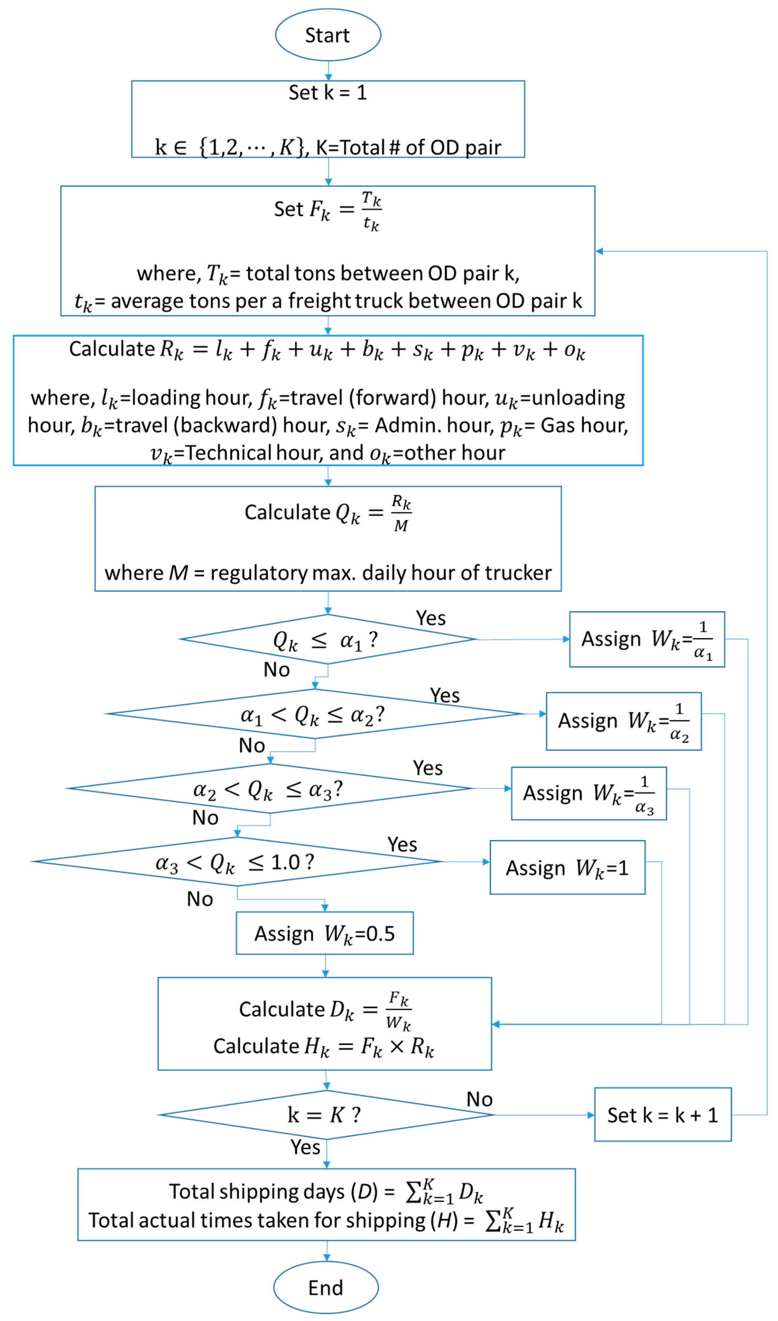
To compare the efficiency values between a truck only system and truck/rail multimodal alternative, we needed to calculate total shipping days needed to move all logs in the database and total actual times taken for truck movements. The flow chart to calculate both parameters is provided in Figure 2.
We first calculated the total trucking frequency ( F k ) needed to deliver all log tonnage between a logging site and a mill for each origin–destination (OD) pair. Then, duration of one round-trip ( R k ) is estimated for each OD pair. A round-trip consists of loading time ( l k ), truck travel time from origin to destination ( f k ), unloading time at destination ( u k ), truck travel time from destination back to origin ( b k ), administration time ( s k ), gas time ( p k ), technical time ( v k ), and “other” time ( o k ). For the definition of each activity within the round trip, we used a similar definition as Lautala et al. [16]. Loading time ( l k ) includes all loading steps in origin, and unloading time ( u k ) indicates time needed for unloading activities in the destination (mill or rail siding). Administration time ( s k ) means time for paperwork, communications with customers or supervisors, and waiting times at the mills and rail sidings, excluding the main loading/unloading actions. Gas time indicates ( p k ) refueling time at gas stations, and technical time ( v k ) means time for any technical activity, such as equipment maintenance, detaching and hooking a trailer, chaining tires, and clearing obstacles from the road. Finally, “other” time ( o k ) means time not allocated in any other category. Those stops included things such as coffee breaks and waiting for other trucks in the forest.
At the next step, the calculated round trip time was used to estimate Q k which is the ratio between round-trip time and the maximum daily operation hours (M) allowed for a log truck driver. This ratio would be the base to estimate how many round trips ( W k ) are possible within the maximum daily operation hours. The α 1 α 3 are constants that express numerical ratios of one round-trip over maximum daily operation hours. In this research, we set up α 1 ,   α 2 ,   and   α 3 as 0.25, 0.33, and 0.5, respectively.
Total shipping days (D) means the number of days needed to deliver all log tonnage between all OD pairs. Thus, it can be calculated as:
D = k = 1 K F k W k
where, K is the total number of OD pairs. Total actual time taken for shipments (H) indicates the hours trucker actually uses for operations. This time can be calculated as:
H = k = 1 K F k × R k
Note that we assumed that drivers can only pick up the second (or third) load from the same location as the first one for the day, so switching to another origin closer to destination in the middle of the day is not allowed. We also did not allow drivers to complete “partial trips”, where the truck gets loaded at the end of day and is taken to destination in the morning.
Finding the round-trip time ( R k ) for each OD used the actual durations of log truck activities. Travel time between OD ( f k and b k ) can be calculated by dividing road distance with average log truck speed in the region. For average truck speed (66 km/h (41 m/h)), loading/unloading times in origin/destination ( l k / u k ), and “other” times ( o k ), we used averages from Lautala et al.’s report [16] that used GPS tracking data and log sheets filled out by the log truck driver in the Upper Peninsula of MI (Table 2).

2.3. Rail Siding Case Studies

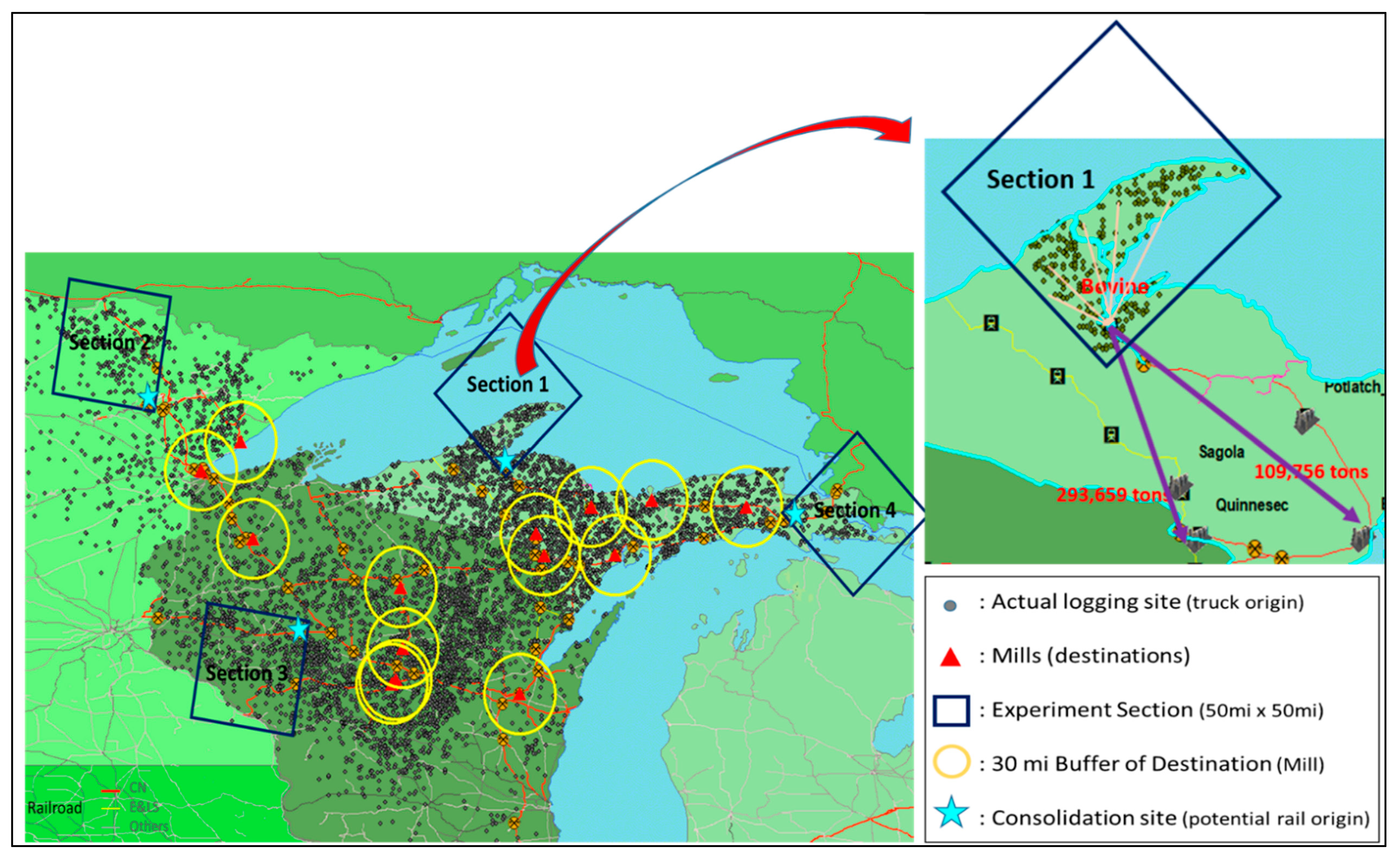
Since investigating all truck movements in the region would be a tremendous task, we selected four log origin areas, each with respective rail sidings as case studies for the investigation (Figure 3). Each section was formed as a 80 km × 80 km (50 m × 50 m) square, extending from the rail siding. All logs that originated within the square were hypothetically trucked to rail siding instead of the mill. The resulting operational parameters were compared with those from actual movements (truck only system). All experimental sections excluded truck shipments that originated within a 48-km (30-m) buffer zone from the destination sites (mills), as it would be unrealistic for the shippers to use rail transportation to replace extremely short-distance truck shipments.
To determine the shipping characteristics of each case study section, we calculated the number of truck origins, total tons shipped, the average distance between truck origins and mills, as well as the average distance between truck origins and the rail siding selected as the collection point. Table 3 summarizes these values for all four case studies. As shown, each section had different average distance between truck origins and destinations (mill or rail siding). For example, Section 4 shows the shortest average distance (53 km) between truck origins and selected rail siding while the average distance to mills was relatively long (227 km). On the other hand, the respective values for Section 2 were quite different (105 km and 208 km).

3. Results

3.1. Results of Log Truck Value Analysis

We calculated time efficiency (the actual time used by log trucks divided by maximum hours of service per day) and the value efficiency (shipped tons per day times loaded kilometers per day) for each section, comparing truck only scenario and multimodal (truck/rail) scenario. Table 4 and Table 5 show the time efficiency and value efficiency for the Section 1 (Bovine, MI, USA), respectively. It should be recognized that the number of trucks was kept the same between the scenarios.
Table 4 shows that by directing all actual log movements by truck from Section 1 to Bovine rail siding, the time efficiency by truckers would slightly increase from 74.5% to 77.1%. The value efficiency, on the other hand, would increase from 8340 t-km to 11,732 t-km that equals 41% increase in average loaded ton-kilometers per day for each log truck (Table 5). More importantly, the empty kilometers per a shipped ton ((c) in Table 5), which indicates average unloaded kilometers created by shipping 1 tonnage of cargo would decrease from 3.58 to 1.27 (64% of reduction rate). This is critical productivity metric, as each empty kilometer decreased the revenues, as the unloaded kilometer only increased expenses (fuel, wear, and tear).
Table 6 summarizes the results of time efficiency and value efficiency analysis for all four case studies. The efficiencies increased in all locations, except Wilpen, MN (Section 2). From Table 3 it can be seen that the average distance to Wilpen rail siding from the log origins was much longer than in other locations (105 km), which explains the efficiency reduction and the logical expectation that obtaining truck benefits is more challenging when origins are located far from the rail siding. Another aspect that impacts the time efficiency and value efficiency is the number of origins. Section 3 (Stanley, WI, USA), which had a comparatively long distance (76 km) between truck origins and rail siding, saw higher efficiency increases than other locations. As Section 3 includes more origins the empty miles could be more easily eliminated, if rail transportation would be combined with trucks. For the reduction rate of average empty kilometers per a shipped ton, it was found that all the sections showed over 40% of reduction from moving from the truck only mode to the truck and rail mode.

3.2. Sensitivity Analysis

Since some of the key parameters were considered fixed in the trucker value analysis, sensitivity analysis on value efficiency were conducted using two key parameters of log truck movements: (1) average truck speed (66 km/h used in the analysis) and (2) maximum hours of service per day by truck drivers (12 h).
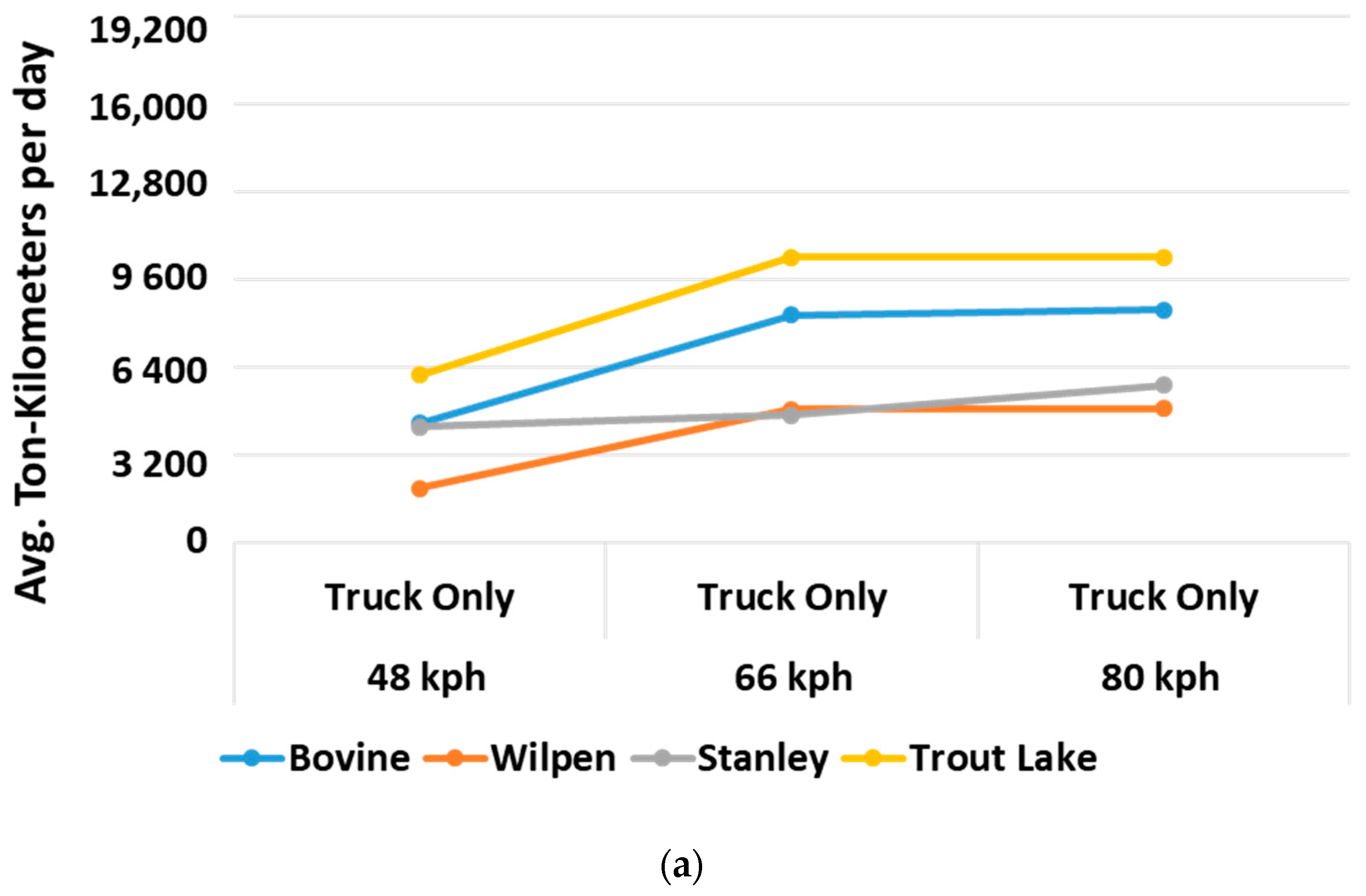
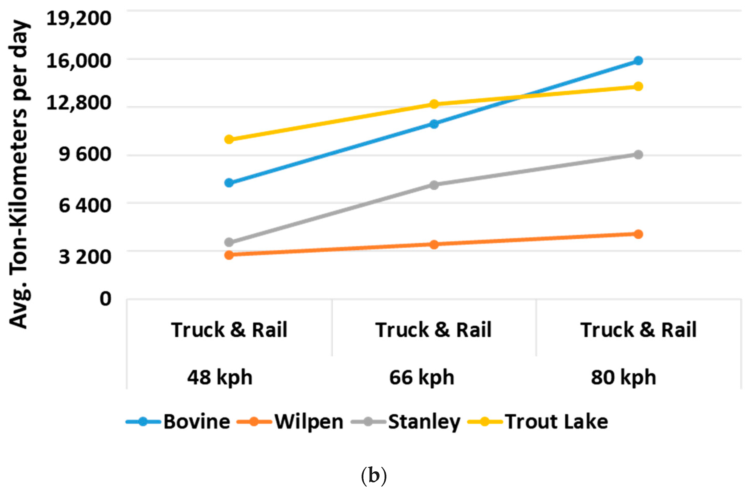
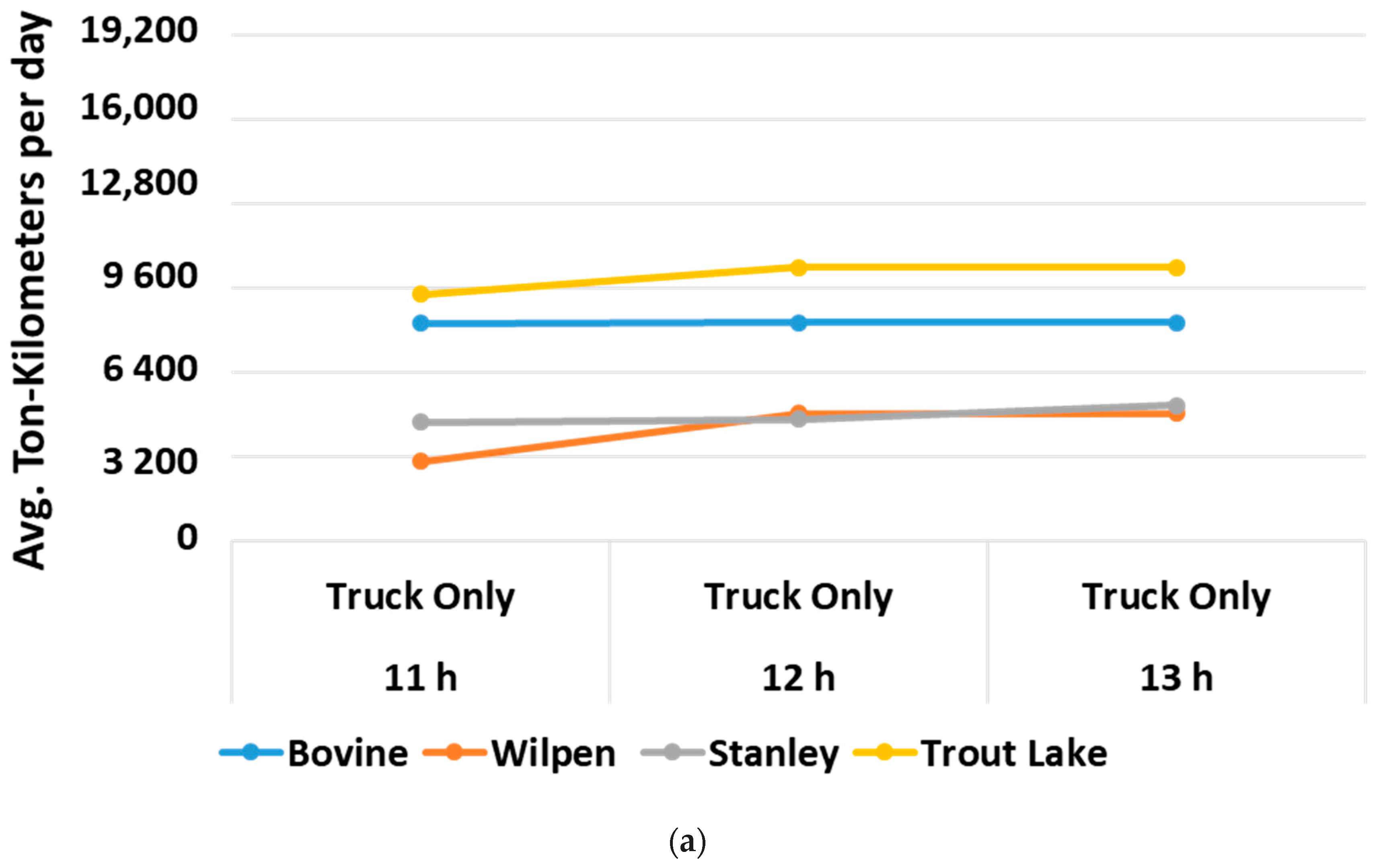
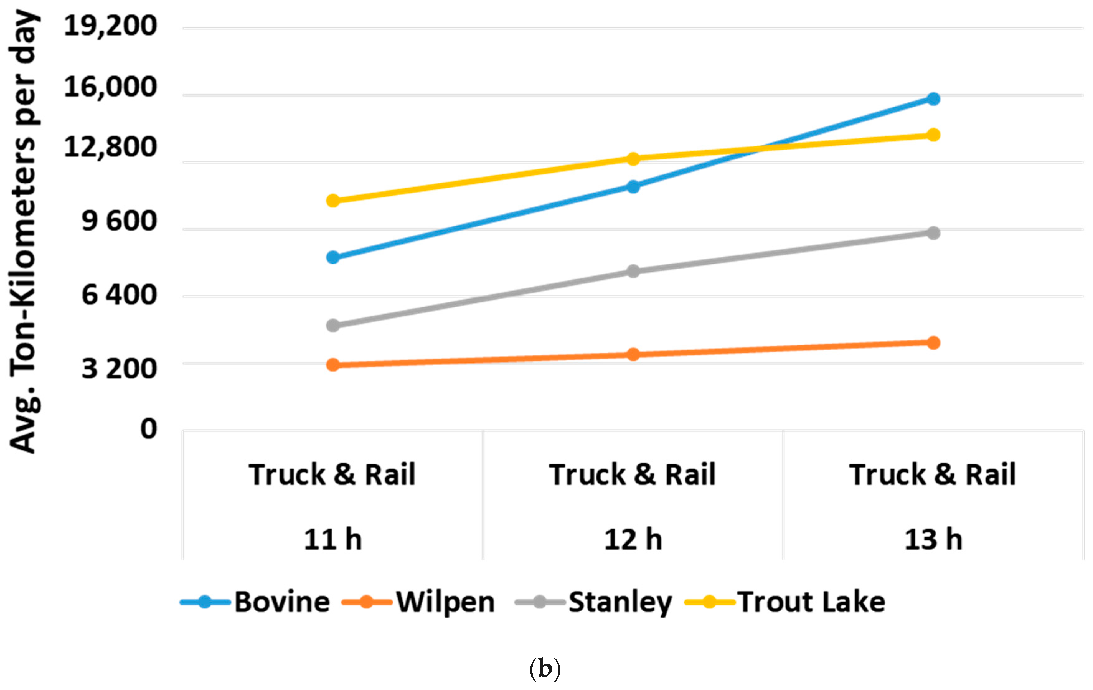
Figure 4 provides the sensitivity analysis results on the various log truck speeds for truck only and multimodal scenarios. As expected, the ton-kilometers per day increased with the increase of truck speeds (4.6% when moving from 66 to 80 km/h average speed), suggesting that increasing truck speeds would improve log truck productivity in general. However, more importantly the productivity increases were greater in the multimodal scenario (Figure 4b), which suggests that increases in truck speed had higher potential to improve the value efficiency if both truck and rail were used (22.6% in multimodal vs. 4.6% in truck only scenario). With shorter round trips, the higher speeds could be more easily converted to additional round trips while remaining within the hours of service limitations.
Figure 5 provides the results for the hours of service sensitivity analysis. Similar to speed, ton-kilometers per day increase with higher hours of service, but the impact is higher in the multimodal scenario (21.4% increase vs. 1.9% increase in truck only, when moving from 12 to 13 h of service; Figure 5). Just like with average speed increases, shorter trips to rail sidings make it easier to add round trip to a daily schedule.

4. Discussion and Conclusions

The trucker value analysis attempted to quantify the potential benefits/disadvantages for log truckers caused by a shift from truck only movements to multimodal truck/rail transportation. We applied actual data collected from the forest products industry companies and truck performance data collected in an earlier study for four case study locations as part of the analysis. The data was preprocessed to improve the accuracy of shipment origins.
Overall, we found that in three out of our four case studies, re-routing log movements through rail yard/siding improved the time efficiency (amount of daily service time used efficiently) and the value efficiency (loaded ton-kilometers per day). In addition, we found that average unloaded kilometers created to ship a ton of log would decrease. A decrease in unloaded kilometers per shipping ton is likely to improve truckers’ economics (they get normally paid in loaded ton kilometers). Equally, the lower unloaded kilometers per shipping ton is likely to benefit truckers, as it can provide more opportunities to generate revenues and a reduction in empty kilometers reduces both fuel consumption and equipment wear. In the one case where such benefits did not materialize, the main reason seemed to be the lower difference between distances to rail siding versus the mill. In the ensuing sensitivity analysis, we found that multimodal transportation received higher gains from increased average truck speed and increased maximum hours or service than in the truck-only system.
Overall, we believe our study to be the first one that uses a detailed and actual freight movement to investigate the impacts of modal shift on the log transportation system. The sponsoring industry companies recognize that any approach that may provide improvements to truckers’ economic health are important, as recruiting/keeping trucks and drivers is a well-known challenge for the industry in the study region. While we did not convert the increase in ton kilometers and in the ratio between loaded and total miles to economic benefits to avoid confidentiality issues in cost data, the companies can take our results to further evaluate the impact of our findings in economic terms.
It should be noted that while the study received unprecedented support from the industry, there were certainly shortcomings/limitations that should be recognized when interpreting the analysis results. First, the analysis relied on parametric values for the daily time consumption breakdown for trucks that were collected from the operational data of a small sample of trucks (five in total). Second, the analysis excluded the time it takes the trucks to arrive to the first loading location of the day from their residences. Third, when analyzing the maximum number of trips per day for each truck, the model allowed drivers to pick up the second (or third) load only from the same location as the first one for the day. It also did not allow drivers to complete “partial trips”, where the truck gets loaded at the end of day and is taken to the final destination in the morning. Finally, we did not include the shipping rates in the analysis, so the impact of the multimodal alternative on the total cost of shipping was left to our industry stakeholders. In addition to addressing the limitations identified above, the future analysis should determine when the additional cost from transloading to the railway could be recovered by reduced rates by truckers (due to more loaded kilometers and less total kilometers per day) and by the railway (due to increased and consistent volumes from the specific siding).

Author Contributions

The authors confirm contribution to the paper as follows: Conceptualization, S.K. and P.L.; Methodology, S.K., P.L. and K.Z.; Software, S.K. and K.Z.; Validation, S.K., P.L. and K.Z.; Formal Analysis, S.K., P.L., and K.Z.; Investigation, S.K. and P.L.; Data collection, S.K. and P.L.; Writing—Original Draft Preparation: S.K.; Writing—Review and Editing, S.K., P.L. and K.Z.; Project Administration, P.L.; Funding Acquisition, P.L. All authors have read and agreed to the published version of the manuscript.

Funding

This research was funded by the Michigan Economic Development Corporation (MEDC), the Michigan Department of Transportation (MDOT), and the US DOT OST-R Tier 1 University Transportation Center, DTRT12-G-UTC18/DTRT13-G-UTC52. Additionally, the APC and the promotional activities of this research were funded by a grant from R&D program of the Korean Railroad Research Institute, Korea.

Acknowledgments

The research team would like to acknowledge the forest product companies associated with LSSA and the two rail carriers (CN and E & LS) who participated in the research.

Conflicts of Interest

The authors declare no conflict of interest. The founding sponsors had no role in the design of the study; in the collection, analyses, or interpretation of data; in the writing of the manuscript, and in the decision to publish the results.

References

  1. Youngs, R.L. Meeting the challenge of change. For. Prod. J. 2007, 57, 6. [Google Scholar]
  2. BTS, U. Average Length of Haul, Domestic Freight and Passenger Modes. 2019. Available online: https://www.bts.gov/content/average-length-haul-domestic-freight-and-passenger-modes-miles (accessed on 30 October 2019).
  3. Meyer, T.; Ernst, A.T.; Krishnamoorthy, M. A 2-phase algorithm for solving the single allocation p-hub center problem. Comput. Oper. Res. 2009, 36, 3143–3151. [Google Scholar] [CrossRef]
  4. Yaman, H. Allocation strategies in hub networks. Eur. J. Oper. Res. 2011, 211, 442–451. [Google Scholar] [CrossRef] [Green Version]
  5. Ishfaq, R.; Sox, C.R. Design of intermodal logistics networks with hub delays. Eur. J. Oper. Res. 2012, 220, 629–641. [Google Scholar] [CrossRef]
  6. Andersen, J.; Christiansen, M. Designing new European rail freight services. J. Oper. Res. Soc. 2009, 60, 348–360. [Google Scholar] [CrossRef]
  7. Pazour, J.A.; Meller, R.D.; Pohl, L.M. A model to design a national high-speed rail network for freight distribution. Transp. Res. Part A 2010, 44, 119–135. [Google Scholar] [CrossRef]
  8. Verma, M.; Verter, V.; Zufferey, N. A bi-objective model for planning and managing rail-truck intermodal transportation of hazardous materials. Transp. Res. Part E 2012, 48, 132–149. [Google Scholar] [CrossRef]
  9. Chang, H.; Jula, H.; Chassiakos, A.; Ioannou, P. A heuristic solution for the empty container substitution problem. Transp. Res. Part E 2008, 44, 203–216. [Google Scholar] [CrossRef]
  10. Bock, S. Real-time control of freight forwarder transportation networks by integrating multimodal transport chains. Eur. J. Oper. Res. 2010, 200, 733–746. [Google Scholar] [CrossRef]
  11. Di Francesco, M.; Lai, M.; Zuddas, P. Maritime repositioning of empty containers under uncertain port disruptions. Comput. Ind. Eng. 2013, 64, 827–837. [Google Scholar] [CrossRef]
  12. DOT, U. Transportation Networks. In Bureau of Transportation Statistics: National Transportation Atlas Database; US Department of Transportation: Washington, DC, USA, 2016. [Google Scholar]
  13. National Renewable Energy Laboratory. Biopower Atlas; National Renewable Energy Laboratory: Golden, CO, USA, 2015.
  14. Sun, G.; Mason, R.; Disney, S. MOVE: Modified Overall Vehicle Effectiveness. In Proceedings of the 8th International Symposium of Logistics, Seville, Spain, 14 July 2003. [Google Scholar]
  15. DOT, U. Hours of Service of Drivers: Final Rule; US Department of Transportation: Washington, DC, USA, 2011.
  16. Lautala, P.; Pouryousef, H.; Stewart, R.; Ogard, L.; Vartiainen, J. Analyzing Log and Chip Truck Performance in the Upper Peninsula of Michigan with GPS Tracking Devices; National Center for Freight and Infrastructure Research and Education (CFIRE): Medison, WI, USA, 2011. [Google Scholar]
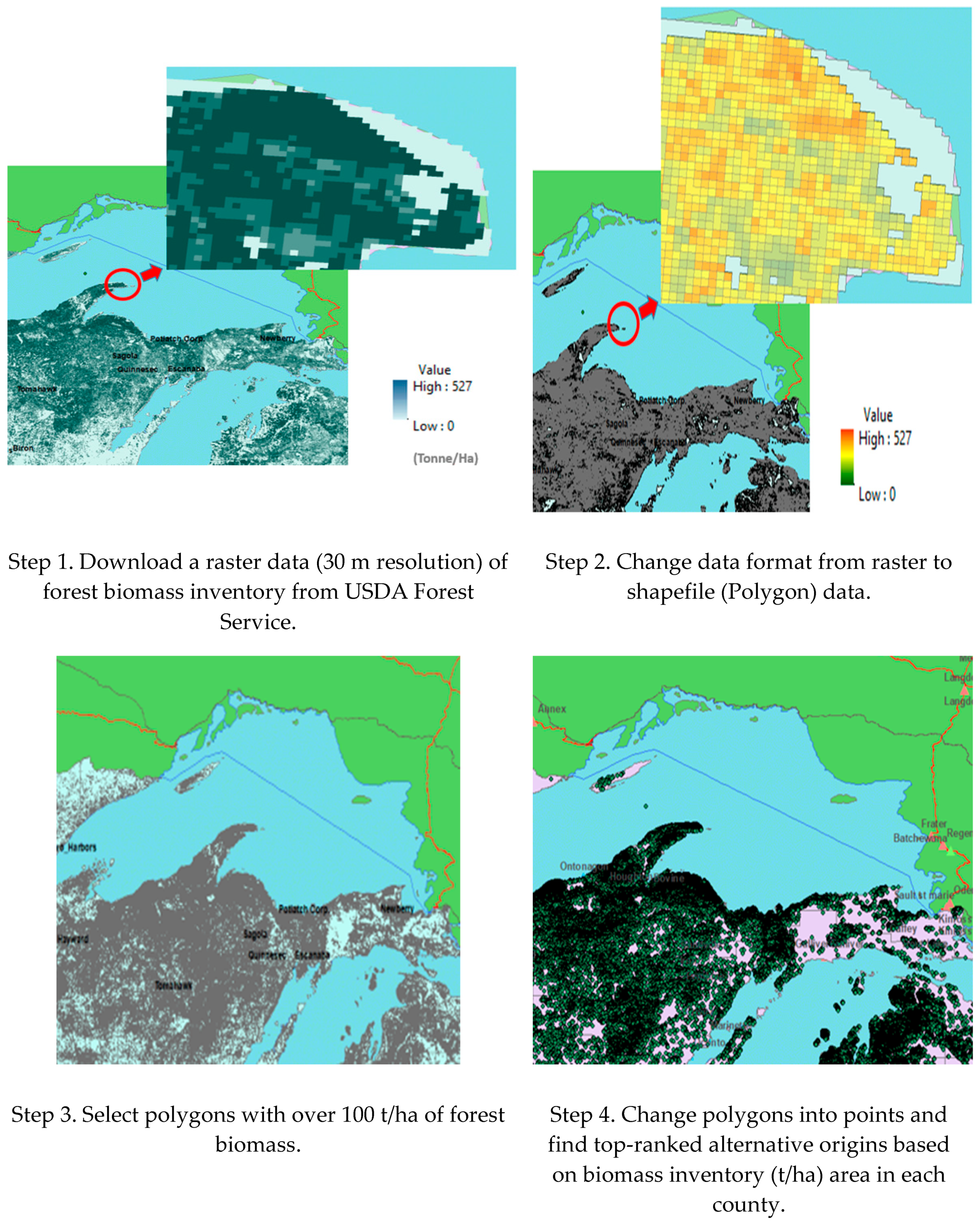
Figure 1. Four-step process used for creating alternative origins for logs.
Forests 11 00677 g001
Figure 2. Truck shipment calculations methodology.
Forests 11 00677 g002
Figure 3. Four case study rail sidings/origin areas for trucker value analysis.
Forests 11 00677 g003
Figure 4. Log truck speed sensitivity analysis results. (a) Truck-only scenario; (b) Multimodal with rail scenario.
Forests 11 00677 g004aForests 11 00677 g004b
Figure 5. Hours of service sensitivity analysis results. (a) Truck-only scenario; (b) Multimodal with rail scenario.
Forests 11 00677 g005aForests 11 00677 g005b
Table 1. Summary of log truck movement data used in this study.
CategorySummary of Log Movement Data
1Number of companies and mills5 companies and their 14 mills
2Total Tonnage:Total log tons = 7,936,027
3Number of ShipmentsIn total 227,715 records of truck shipment data
4Number of Origins/DestinationsOrigins (log landings/yards): 8206/Destinations (mills): 14
5Time Period2017 (January–December)
6Study AreaWI, MN, and UP of MI in the US
7InfrastructureActual road network provided by US DOT
8Geographic coordinates systemLatitude and Longitude(Preprocessing: Modification to Latitude/Longitude)
Table 2. Average stop time of log trucks by activity (hours) [16].
ActivityAdministrationTechnicalGasOtherLoadingUnloading
Avg. stop time (hours)0.070.360.120.261.350.65
Table 3. Summary of case study characteristics.
Rail Siding# of Truck OriginsAvg. Distance between Truck Origins and Mills (Destinations)Avg. Distance between Truck Origins and Rail SidingTotal Shipping Tons
Section 1Bovine, MI, USA207216 km60 km247,896 t
Section 2Wilpen, MN, USA212208 km105 km83,685 t
Section 3Stanley, WI, USA320164 km76 km114,402 t
Section 4Trout Lake, MI, USA121227 km53 km93,509 t
Table 4. Time efficiency for the Section 1 (Bovine, MI, USA).
RouteShipped TonsDays (a)Available Time for Shipping ((b) = 12 h × (a))Actual Time Taken for Shipping ((c) = Used Hours × (a))Time Efficiency ((c)/(b))
(1) Truck + Rail ScenarioFrom Forest to Bovine247,896 t2580 days30,960 h23,866 h77.1%
vs.
(2) Truck only ScenarioFrom Forest to Mill247,896 t5130 days61,560 h45,847 h74.5%
Table 5. Value efficiency for the Section 1 (Bovine, MI, USA).
RouteShipped Tons per Day
(a)
Loaded KilometersLoaded Kilometers per Day (b)Total Kilometers per DayAvg. Loaded Ton-Kilometers per Day ((a) × (b))Avg. Empty Kilometers per Shipped Ton (c)
(1) Truck + Rail ScenarioFrom Forest to Bovine96.1 t314,986 km122.1 km244.1 km11,732 t-km1.27 km
vs.
(2) Truck Only ScenarioFrom Forest to Mill48.3 t885,472 km172.7 km345.2 km8340 t-km3.58 km
Table 6. Case study results of time efficiency and value efficiency.
Time EfficiencyValue Efficiency
(Avg. Ton-Kilometers Per Day)
Rail SidingBefore: Truck OnlyAfter: Truck and RailChange (Before/After)Before: Truck OnlyAfter: Truck and RailChange (Before/After)
1Bovine, MI, USA74.5%77.1%2.6%p↑8340 t-km11,732 t-km41%↑
2Wilpen, MN, USA82.1%65.7%16.4%p↓4875 t-km3671 t-km25%↓
3Stanley, WI, USA64.8%81.3%16.5%p↑4664 t-km7657 t-km64%↑
4Trout Lake, MI, USA78.4%87.5%9.1%p↑10,454 t-km13,063 t-km25%↑