Article

Mapping the Decay Hazard of Wooden Structures in Topographically Divergent Regions

Wood Biology and Wood Products, University of Goettingen; Buesgenweg 4, D-37077 Goettingen, Germany
*
Author to whom correspondence should be addressed.
Forests 2020, 11(5), 510; https://doi.org/10.3390/f11050510
Submission received: 25 March 2020 / Revised: 21 April 2020 / Accepted: 27 April 2020 / Published: 1 May 2020

Abstract

:
The service life of exposed wooden structures depends on many endogenous and exogenous factors with moisture being key for fungal degradation. Climate parameters are therefore important input variables for modelling fungal decay in wood. In recent years, different approaches aimed at modelling climate-induced dosage on the material climate (i.e., exposure models) and the effect of the latter on fungal decay (i.e., decay models). Based on maps of Europe, North America or Australia, the decay hazard can be assigned to zones and used for estimating the relative decay potential of an arbitrary location. However, especially in topographically divergent regions, the climate-induced decay hazard can vary strongly within a small area. Within this study, decay hazards were quantified and mapped for a mountainous region where topography-induced differences in local climate and corresponding exposure dosage can be expected. The area under investigation was Switzerland. In addition to the Scheffer Climate Index (SCI), two exposure models were combined with two decay models and used to quantify the relative moisture- and temperature-induced exposure dose at 75 different weather stations in Switzerland and adjacent regions. The exposure was expressed as relative dosage with Uppsala (Sweden) as a reference location. Relative dose values were calculated for locations between weather stations using an ‘inverse distance weighted (IDW)’ interpolation and displayed in maps for the entire country. A more detailed analysis was undertaken for the Lötschental area, which is the largest valley on the northern side of the Rhône valley in the canton of Valais. The relative dose differed strongly within small areas and altitude was well correlated with the average annual temperature and the resulting relative dose. It became evident that small-scale mapping with high resolution is needed to fully reflect the impact of topography and other local conditions on the moisture- and temperature-induced decay risk in wooden components.

1. Introduction

The service life of exposed wooden structures depends on many endogenous and exogenous factors, with moisture being key for fungal degradation. Climate parameters are therefore important input variables for modelling fungal decay in wood and decay hazard mapping can help to estimate exposure-related dosage in a quantitative manner [1]. Pioneering work on decay hazard mapping was carried out by Theodore Scheffer in the early 1970s. Scheffer [2] suggested a climate index to correlate climatic data with the site-specific potential for biological decay. The hazard potential of different climates in the USA was estimated by empirically determined decay intensity from field tests at four different locations. In this early attempt the focus was on the parameters ‘temperature’ and ‘distribution of rainfall’, which Scheffer described as follows:
Scheffer Climate Index   ( SCI ) = Jan Dec [ ( T 35 ) ( D 3 ) ] / 30   [ - ]
where T is the mean day temperature of the month [°F], and D is the mean number of days with more than 0.001 inch of rain per month [-].
The higher the SCI, the higher is the hazard for decay with values between 0.0 for Yuma, Arizona, and 137.5 for West Palm Beach, Florida, for the continental part of the USA. The SCI has been used for decay hazard mapping of various countries and regions such as Canada [3], North America [4], Korea [5,6], China [7], Japan [8], Australia [9], Norway [10], Spain [11], Greece [12], Northern Europe [13] and Europe [14,15]. Finally, Carll [16] published a revised hazard map for the United States using climate data from 1971–2000 and showed that climate-induced decay hazard had changed over the years in some regions.
According to Carll [16], the SCI is a “metric by which relative hazard can be compared between geographic locations, the SCI is not intended to predict decay propagation rate nor time to failure in specific constructions”. This particularity is not necessarily a limitation of the approach, but has been controversially discussed (e.g., [11,17,18,19,20,21]). However, beyond doubt, the SCI is still the most often used index of its kind for estimating the relative climate-induced decay hazard of geographical locations [22,23,24,25,26].
Alternatively, other climate indices have been proposed and considered for service life planning (e.g., [27,28,29,30]), but suffered from insufficient fit between macro-climatic data and decay rates [19,24,31,32].
Within the European research project WoodExter, an attempt was made to utilize a decay model for generating a decay hazard map of Europe [33]. Based on laboratory test results, the parameters relative humidity (RH) and temperature (T) were used to predict mass loss (MLF) caused by decay fungi. The physiological needs of brown rot fungi were studied by Viitanen and co-workers [34,35,36]. Based on their findings, a so-called set-back model was developed using RH and T as input variables. Decay development was modelled as two processes: an activation process and a mass loss process [33,37]. A parameter, α, was defined as a relative measure of the state of the fungus with respect to its state at the initiation of the mass loss process. It is initially 0 and grows gradually to a limit of 1, at which the mass loss process is initiated. Both processes have been modelled and the MLF in Scots pine sapwood (Pinus sylvestris) after ten years of above-ground exposure was predicted and mapped for Europe.
Dose–response models for predicting fungal decay in above-ground situations were developed based on long-term field test data by different authors [20,32,38]. They all used wood moisture content (MCw) and temperature (Tw) as input variables and a five-step decay rating according to EN 252 [39] between sound (0) and failure (4) to specify different limit states. The models differed with respect to the range of MCw and Tw in which a daily dose was allowed to occur, but had in common that no dose occurs when at least one dose component was 0. In previous steps, MCw and Tw can be calculated with the help of empirical or numerical exposure models based on weather data such as precipitation, air temperature (T) and RH (e.g., [13,15]). Consequently, linking an exposure model with a decay model allows for the prediction of the decay hazard within a wooden component and thus, its expected service life for a given design and material under given use conditions [40]. Furthermore, the decay hazard for an arbitrary location can be calculated and expressed as annual dose, i.e., the cumulated daily dose during one normal year. The first decay hazard maps for Europe based on combined exposure and decay models were presented by Brischke et al. [14] and Frühwald Hansson et al. [41]. Both showed that differences in the relative decay hazard exist within Europe, but were dependent on the models applied. In general, most severe exposure was expected in the oceanic influenced regions of coastal UK, Ireland, and Norway, whereby the cold and dry regions of the Nordic countries as well as the arid Mediterranean regions revealed the lowest decay potential. However, besides these general tendencies, numerous regional ‘hot and cold spots’ were observed. Consequently, drawing borders between different decay hazard zones within Europe appeared difficult, since the climate-induced influences may change locally very much. Furthermore, model-specific differences occurred, especially for dry sites, where higher doses were found when using a more moisture-sensitive decay model. It is therefore hypothesized that local deviations from the general hazard distribution and its gradients within the continent can be attributed to landscape features such as lakes, rivers, and mountains.
This study is therefore focusing on the effect of topography on the moisture- and temperature-induced decay hazard of timber structures. We aimed at quantifying and mapping the decay hazard for a mountainous region where topography-induced differences in local climate and corresponding exposure dosage were expected. The area under investigation was Switzerland and different combinations of exposure and decay models were applied.

2. Materials and Methods

2.1. Investigation Areas and Data Source

The area under investigation was the entire country territory of Switzerland (Figure 1a), and for a detailed analysis the Lötschental area (Figure 1b), which is the largest valley on the northern side of the Rhône Valley in the canton of Valais. It lies in the Bernese Alps, with the Lonza River running down the length of the valley from its source within the Long Glacier.
Two exposure models were combined with two decay models and used to quantify the relative moisture- and temperature-induced exposure dose at 75 different weather stations in Switzerland and adjacent regions representing an altitude range between 103 and 3580 m. In addition, the Scheffer Climate Index (SCI, [2]) was determined for each location. Meteorological data were taken from the Meteonorm database [44] and typical years were calculated based on averaged month-values.
For analyzing differences in decay hazard in the Lötschental area, weather data were used from 276 locations in grit patterns of 2.5 × 2.5 km, 5.0 × 5.0 km, and 7.5 × 7.5 km. The altitude in the Lötschental area was between 623 and 3967 m.

2.2. Exposure Models

Two different exposure models were used to predict the wood moisture content MCwood in a reference wooden component, i.e., a horizontal board (cross section 22 × 90 mm2) made from Norway spruce (Picea abies) without any water trapping (see also [32]). Exposure model 1 (EM 1), as described by Niklewski et al. [13], refers to a depth of 11 mm (mid thickness of the board). MCw was calculated based on RH and T as follows:
M C w ( R H ,   T ) = 10.17 + 0.122 R H 0.275 T   [ % ]
where MCw is the wood moisture content [%], RH is the relative humidity [%], and T is the air temperature [°C]. Rain was only implicitly considered by setting the RH to 100 % during rain.
The second empirical exposure model (EM 2) was based on the test results reported by Tveit [45] and Van den Bulcke et al. [46] and is described in detail by Frühwald et al. [41]. Moisture content, MCw, depends on RH and is calculated as follows:
M C w ( R H ) = 0.7 R H 3 0.8 R H 2 + 0.42 R H + 0.0077   [ % ]
where MCw is the wood moisture content [%], and RH is the relative humidity [%].
The MCw, in equilibrium with RH, was estimated on the basis of the average value of RH for two full days. This is assumed to account for a certain delay corresponding to diffusion of water into the wood. Additionally, MCw is increased by rain events. For each 24-h period it is assumed that rain occurs if the accumulated rain is at least 4 mm. A rain period is then defined as an uninterrupted sequence of 24-h periods with rain. The duration of a rain period is denoted tr. A drying period is defined as the time after a rain period during which the MCw returns to equilibrium with ambient RH. The duration td of the drying period depends on the length tr of the rain period. Based on measurements on plywood (Van den Bulcke et al. 2009), the drying duration can be estimated as:
t d a · t r   [ % ]
where a is an empirical parameter of the order 2–3. Here, a = 2.5 was used.
Undoubtedly, this rough value does not give completely exact results. However, more exact results were not necessary, as the daily rain accumulated during 24 h was used in the model, disregarding when during that 24 h period the rain period occurred. For each day i with rain, the daily average MCw,1 (ti) was calculated according to Equation (5) where kr is the relative increase of MCw due to rain. According to data by Van den Bulcke et al. [46], kr is in the range of 0.3 to 1.5 for different plywood samples using hardwood and softwood species, and different lengths of rain events. In general, the longer the rain event, the higher is the observed MCw increase. In the present paper kr = 0.8 was used.
M C w , 1 ( t i ) = M C w , 01 ( t i ) · ( 1 + k r )   [ % ]
At the end of each rain period tr and td = a∙tr were determined as well as the difference ΔMCw,1r between RH- and rain-induced MCw, shown in Equation (6). Here, te denoted the last day of the rain period.
Δ M C w , 1 r = M C w , 1 ( t e ) M C w , 01 ( t e ) = k r · M C w , 01 ( t e )   [ % ]
For day k after a rain period, the MCw was determined as:
M C w , 1 ( t k ) = max [ ( M C w , 1 ( t k 1 ) k t d Δ M C w , 1 r ) , M C w , 01 ( t k ) ]   [ % ]
Note that as soon as a new day with rain occurred, the MCw was again determined by Equation (5).

2.3. Scheffer Climate Index (SCI)

The Scheffer Climate Index was determined according to the following equation.
Scheffer Climate Index   ( S C I ) = Jan Dec [ ( T 2 ) ( D 3 ) ] / 16.7   [ - ]
where T is the mean day temperature of the month [°C], and D is the mean number of days with more than 0.25 mm of rain per month [-]. Note: Negative monthly values were set as zero to avoid negative SCI values. With this climate index, Scheffer [2] distinguished three climate zones in the USA, according to SCI < 35, 35 ≤ SCI < 65 and SCI ≥ 65. The higher the SCI, the higher the decay hazard.

2.4. Decay Models

Decay models describe the degradation of wood due to fungal decay. The SCI can be seen as a simplistic decay model with output in terms of relative decay hazard. More sophisticated models aim to describe the output in physical quantities such as mass loss or decay rate [13]. In this paper, two so-called dose–response models from Isaksson et al. [32] were used and combined with the above-mentioned exposure models: the logistic model (LM) and the simplified logistic model (SLM).
Doses were accumulated at a rate which is determined based on the daily average material climate (MCw, Tw), the maximum dose being one per day which represents optimal conditions for decay. The daily dose at day i, here denoted di, is a function of two components: the wood temperature-induced dose, dT, and the moisture-induced dose dMC, calculated from the daily average temperature T and the daily average moisture content MCw, respectively. Both components are required to be above zero for a dose to be produced. The total dose was the cumulative sum of daily doses from day 1 to n according to:
d ( t ) = i = 1 n d i ( d M C ( M C w ) , d t ( T w ) )   [ d ]
The end of the specimens’ service life occurred when the accumulated dose d(t) exceeded the critical dose dcrit and the service life was defined by the corresponding amount of days n. The critical dose dcrit was defined by the dose which corresponds to a certain level of decay, in this case decay rating 1, 2, 3 or 4 [39].

2.4.1. Logistic Dose–Response Model LM

A total daily dose, which impacts on the wood, was assumed to be a function of dMC and dT. Starting from the literature data, the cardinal points of the parameters Tw and MCw for fungal decay were sought and used to set up polynomial base functions for both dose components (Equations (10) and (11)). The total dose di was then calculated as a function of dMC and dT according to Equation (12), where dT was weighted by a factor a.
d M C ( M C w ) = { 0 i f   M C w < 25 % e · M C w 5 f · M C w 4 + g · M C w 3 h · M C w 2 + i · M C w j i f M C w 25 %
d T ( T w ) = { 0 i f   T w , m i n <   0   ° C   o r   i f   T w , m a x   > 40   ° C k T w 4 + l T w 3 m T w 2 + n T w i f   T w , m i n     0   ° C   o r   i f   T w , m a x   <   40   ° C
D = ( a · d T [ T w ] + d M C [ M C w ] ) · ( a + 1 ) 1 i f d M C > 0   a n d   d T > 0
where D is the dose [d], dT is the temperature-induced dose component [-], dMC is the moisture-induced dose component [d], MCw is the wood moisture content [%], Tw is the daily average wood temperature [°C], Tw,min is the minimum wood temperature for the day considered [°C], Tw,max is the maximum wood temperature for the day considered [°C], a is the temperature weighting factor, and e, f, g, h, I, j, k, l, m, n are variables.
The best fit for this model against the available data was obtained with the parameters listed in Table 1 and the final logistic model function according to Equation [13].
The total dose over a certain time period is given by Equation [13] and the decay rating is given by the dose–response function:
D R ( D ( n ) = 4 · E X P ( E X P ( 1.7716 ( 0.0032 · D ( n ) ) ) )   [ % ]
where DR is the decay rating according to EN 252 [39], and D(n) is the total dose for n days of exposure.

2.4.2. Simplified Logistic Dose–Response Model SLM

Again, the limit state function was based on a dose–response model, where the dose is given as a function of MCw and Tw, but here the dose D was assumed to be the product of the two dose components dMC and dT. The second simplification refers to dMC and dT, which were expressed as a square function and a linear function, respectively [31].
D = d M C ( M C w ) · d T ( T w )   [ % ]
d M C ( M C w ) = { ( M C w / 30 ) 2       i f   M C w 30   % 1                                             i f   M C w > 30   %
d T ( T w ) = { 0 i f   T w < 0 ° C T w / 30                     i f   0 ° C T w 30 1     i f   T w > 30 ° C ° C
where D is the dose [d], dT is the temperature-induced dose component [-], dMC is the moisture-induced dose component [d], MCw is the wood moisture content [%], Tw is the daily average wood temperature [°C].
In contrast to the LM, this simplified approach gave non-zero dose values for MCw below 25% and allowed the moisture dose to give values also for low MCw to be able to specify the “distance to the risk”, but also the uncertainty in MCw measurements and the potential moisture gradients within one wooden component.
The total dose over a certain time period is given by Equation (9) and the decay rating is given by the dose–response function:
D R ( D ( n ) ) = 4 · exp ( exp ( 1.9612 ( 0.0037 · D ( n ) ) ) ) [ - ]
where DR is the decay rating according to EN 252 (2015), and D(n) is the total dose for n days of exposure.

2.5. Decay Hazard Mapping

All 70 Swiss weather stations available via the Meteonorm database [44] were used as well as data from the nearby locations Freiburg (DE), Innsbruck (A), Bolzano (I), Milano (I) and Mâcon (F) for interpolating dose values of the entire territory of Switzerland. The Swedish city of Uppsala served as reference location as previously reported (e.g., [14]). Maps were generated using ArcGIS 10.2 (Esri, Switzerland) based on daily values derived from hourly values in the database. For each model combination (i.e., EM1/LM, EM1/SLM, EM2/LM, and EM2/SLM) annual dose values were calculated and related to the annual dose for Uppsala. In the different maps, the relative dose was displayed.
Each location was captured in the WGS84 system with help of its coordinates and displayed as dot. The relative dose for any location between the weather stations was calculated using the ‘inverse distance weighted (IDW)’ interpolation method. Relative dose values were assigned to twelve classes between zero and three, each with a class size of 0.25. A more detailed analysis was carried out for the Lötschental area with in total 276 locations. The latter were selected systematically to achieve data point grits with different resolution.

3. Results and Discussion

3.1. Switzerland

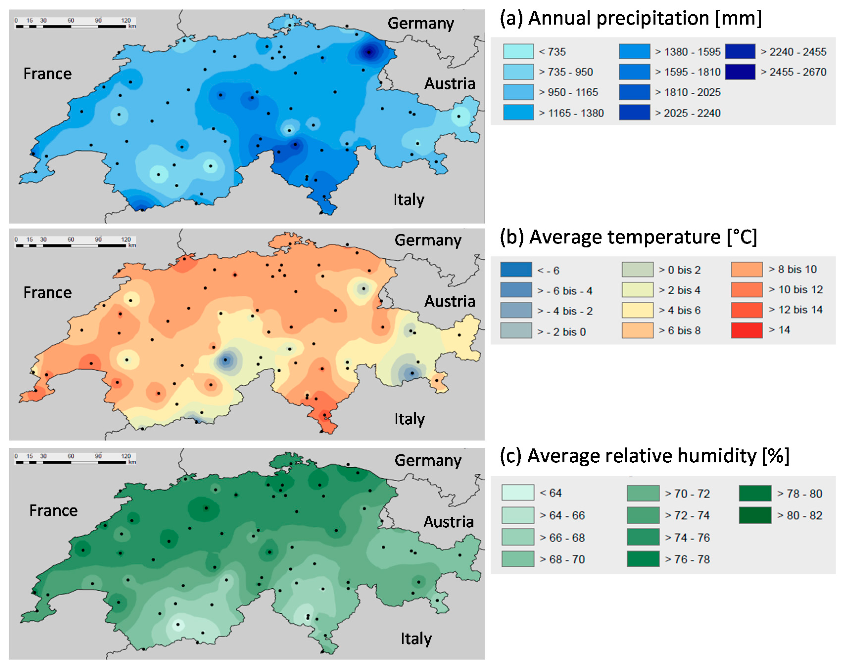
The annual precipitation, the average temperature and the average relative humidity (RH) have been mapped and are shown in Figure 2. Annual precipitation varied between 554 (Sion and Bolzano) and 2680 mm (St. Gallen), but in large areas it was between 950 and 1380 mm (Figure 2a). The average temperature was between −6.7 °C at Jungfraujoch and 12.9 °C in Bolzano; often it was between and 10 °C (Figure 2b). In contrast to annual precipitation and annual average temperature, the annual average RH showed a clear gradient from North to South with an overall range between 62% (Evolene-Villaz) and 79% (Wynau, Figure 2c).
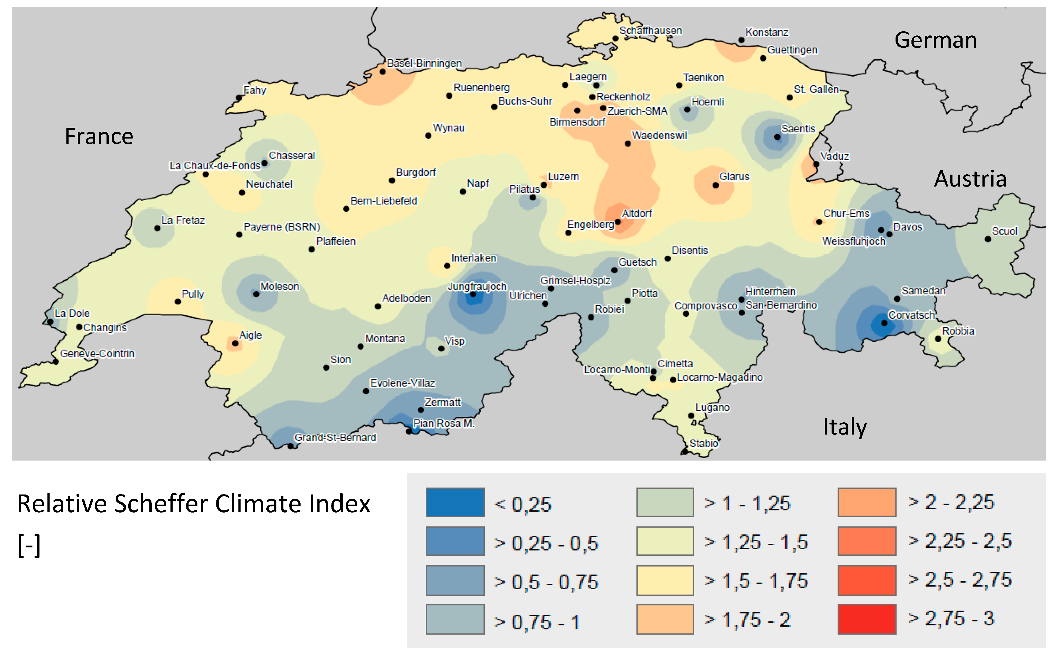
The Scheffer Climate Index (SCI) in Switzerland varied between 0.00 at Jungfraujoch and Pian Rosa at an altitude of 3580 and 3488 m, respectively, and 73.2 in Altdorf (449 m). The latter is also the only location within the highest hazard zone as defined originally by Scheffer [2]: least favourable conditions for decay (SCI < 35), intermediate conditions (35 ≤ SCI ≤ 65) and conditions most conductive for decay (SCI > 65). The relative SCI is shown in Figure 3, with the Swedish city of Uppsala being the reference location at an absolute SCI of 46.3. The relative SCI in Switzerland can be below 0.25 at very high altitudes and above 2.00. Thus, the SCI range within the country is rather high, but extremes are mainly attributed to low temperatures in mountainous areas. Niklewski et al. [15] reported SCI values varying between 17.5 and 70 all over Europe, but with higher values up to 100 in Ireland, North-West Spain and the Southern Balkan. In a study by Brischke et al. [14], the index ranged between 81.0 in Southwest France and 3.9 in Northern Norway, and 5.6 in Romania, respectively. Compared to the entire European continent, the climate-induced hazard within Switzerland varies a lot.
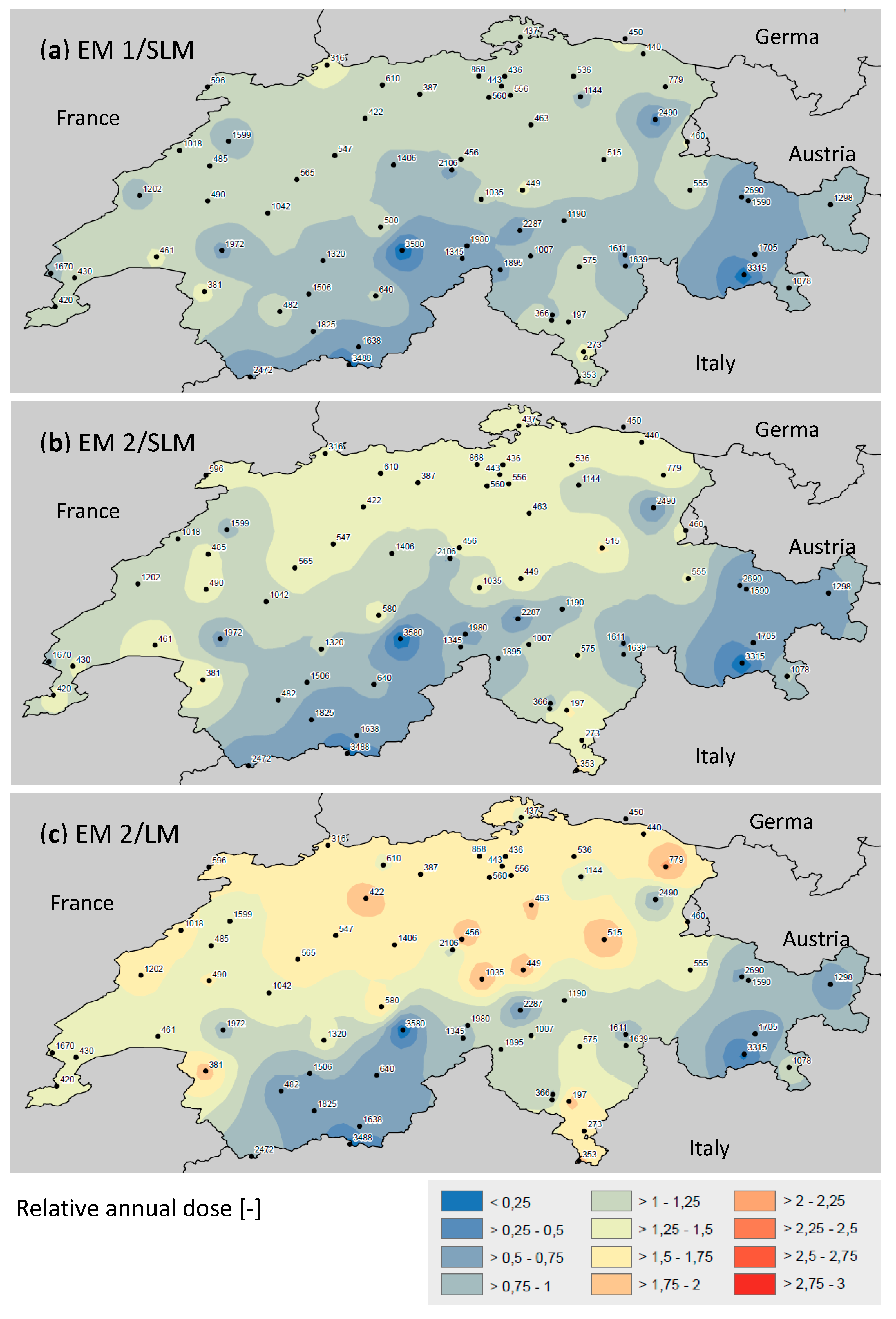
The variation of the site-specific and climate-induced decay hazard in Switzerland became also evident from mapping the annual temperature- and moisture-induced dose which is illustrated in Figure 4 for different combinations of exposure and decay models.
Solely, the EM 1 combined with LM did not allow to distinguish between different locations since the annual dose was ‘zero’ in each place, since the EM 1 led to wood MC almost always below 25%, which is the lower threshold for a moisture-induced dose dMC according to LM. Wood MC > 25% was reached only in winter when temperature was below the freezing point and thus no temperature-induced dose dT occurred. Since the model combination EM 1/LM could not differentiate site-specific decay hazards, it was not further considered within this study.
Generally, the SLM led to less pronounced differences in decay hazard compared to the LM, since only the latter requires wood MC above 25% to account for a moisture-induced dosage, what can be achieved when using the EM 2 and accounting for rain events. In contrast, the SLM accounts for a moisture-induced dose already below 25%, but differences in wood MC in the hygroscopic range, i.e., without any impact of rain events, play only a minor role for wood that is freely exposed to the weather.
A dose gradient became apparent for all three model combinations, but was differently prominent (Figure 4). The strongest gradient was observed for EM 2/LM followed by EM 2/SLM and EM 1/SLM. However, all three maps showed that the Tessin region in the central South of Switzerland showed a higher relative dose, which was against the general southward gradient, but can still be explained by the average temperature which increased southwards in the Tessin region (Figure 2b). Similarly, the average air temperature increased from North to South as shown in Figure 2b, but also ‘hot and cold spots’ became evident where the relative dose was remarkably higher or lower on a small scale compared to adjacent regions. The latter might be induced by differences in altitude and thus the topography.
The climate characteristics precipitation, air temperature and RH as well as the altitude were therefore correlated with the climate-induced dosage. The obtained degrees of determination R2 for a linear fitting curve are summarized for all model combinations and the relative SCI in Table 2. Neither precipitation nor RH were correlated with any of the dose parameters, but altitude and average temperature were. The combinations between exposure models and the SLM-based dosage were highly correlated (R2 = 0.8302 − 0.9953), but also SCI and EM 2/LM were well correlated with both altitude and temperature (R2 = 0.4778 − 0.6893). Altitude, which in turn was highly correlated with the average temperature (R2 = 0.9456), served generally as good indicator for the climate-induced dose.
Mapping SCI (Figure 3) and the relative dose based on EM 2/LM (Figure 4) revealed the highest similarity, which might be due to the same input parameters, i.e., temperature, precipitation, and RH, but became only partly evident from an attempt to correlate both measures (R2 = 0.6453). However, as previously reported by different authors [11,20,22,47], both attempts can be used to predict the performance of wood exposed outdoors under situations referring to the European use class 3.2 [48], which refers to wood exposed to weather, but without permanent contact with soil or water. Here, an accumulation of water in wood shall be expected, although it is spatially limited.
On country level, it became evident that topography—here mainly expressed as altitude—has a major impact on the climate-induced decay hazard of different locations in Switzerland. It was therefore assumed that those become even more pronounced in mountainous regions on a smaller scale.

3.2. Lötschental

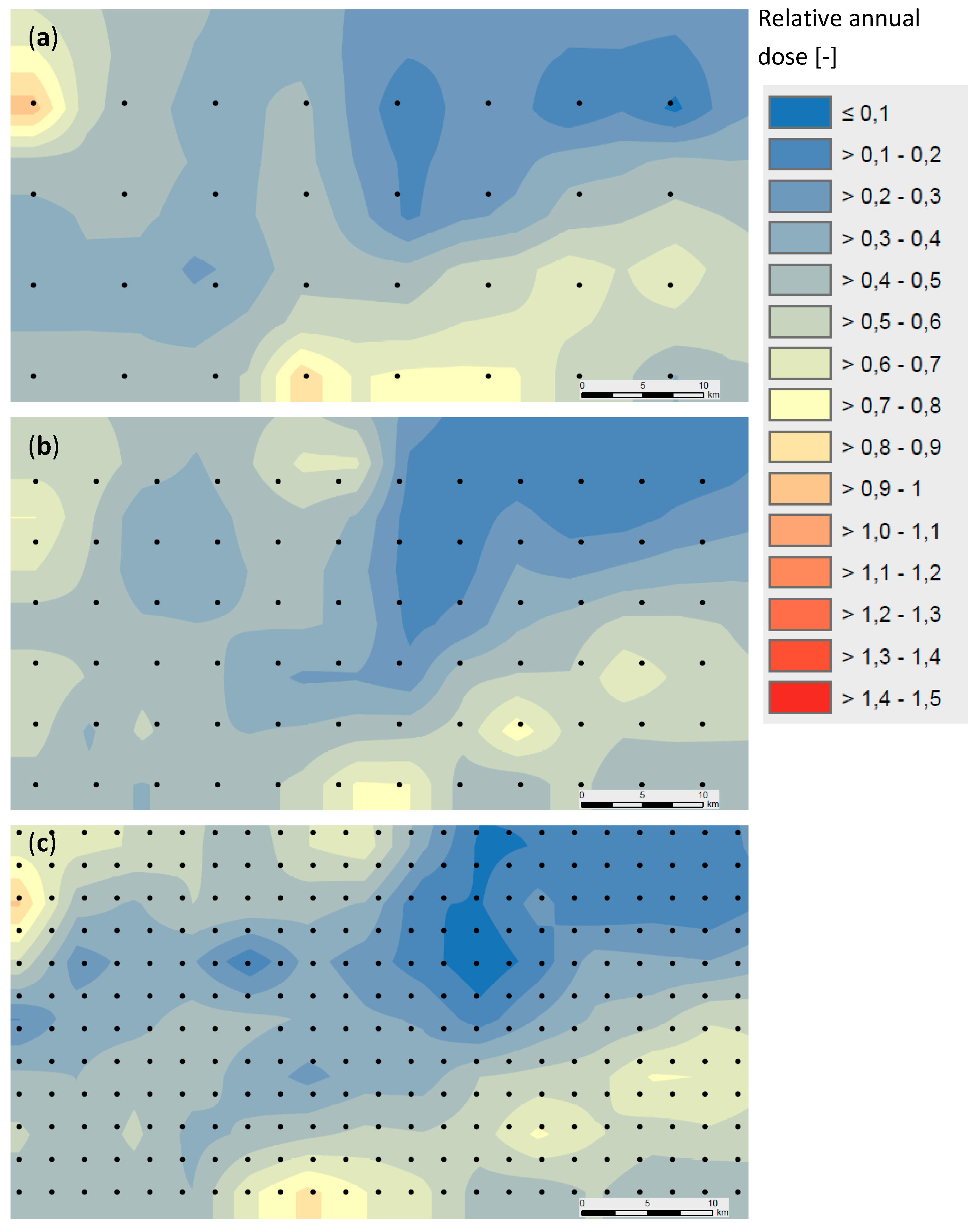
The relative dose was mapped for the Lötschental area in different resolutions. For this purpose, locations were selected in a uniform grid pattern of 7.5 × 7.5 km, 5.0 × 5.0 km, and 2.5 × 2.5 km as shown for EM 2/SLM in Figure 5 and for EM 2/LM in Figure 6. We changed the previously used 12 relative dose classes of 0.25 (e.g., Figure 4) to 15 classes of 0.1 to better illustrate small-scale differences of the decay hazard.
The maximum span of relative decay dose within the Lötschental area increased only slightly with increasing resolution, but dosage was assigned to locations more accurately on a small scale. In particular, the borders between the Long Glacier and the Rhône valley became apparent as well as the Lötschental which follows the Lonza River. With increasing resolution of the maps, the impact of topography on the decay hazard became better visualized. Furthermore, systematic errors became evident when calculating the site-specific dose on the basis of interpolated climate data. The more distinct the topography was, i.e., the higher the differences in altitude, the bigger the error. The latter can be seen, for instance, at the glacier top for which a maximum dose has been assigned only at the highest resolution of 2.5 × 2.5 km.
For a reliable service life prediction of wooden components, it is essential to quantify the climate-induced hazard as accurately as possible [1]. Therefore, different climate levels can be distinguished as follows: macro-, meso-, local, and micro-level. Recently, Emmerich and Brischke [49] showed that at least the latter is influenced by topography, forest cover, and other features that have an impact on characteristic weather parameters such as rain, wind, and solar irradiation. In different, partly ongoing studies, the effect of building design, vegetation and adjacent buildings on moistening and re-drying of wooden building components is examined and quantitatively assessed [40,50]. However, the effect of topography itself can be accounted for through high-resolution mapping of decay doses as exemplarily shown in this study. Alternatively, the site-specific dose can be calculated on the basis of meteorological data bases and existing models to predict exposure dose and resulting decay.
Interestingly, topography-related differences in decay dose became more apparent with increasing resolution for the model combination EM 2/SLM compared to EM 2/LM, which contradicts previous findings on country level (see Figure 4) where the use of the LM led to higher differences in relative decay dosage, but can be explained by different scales used for the analysis, i.e., ≤0.1 to >1.4–1.5 in the Lötschental area (Figure 5 and Figure 6, but <0.25 to >2.75–3.0 for Switzerland (Figure 4).
The overall suitability of a decay prediction model, or a combination of an exposure model and a decay model, respectively, is defined by its predictive power [1]. Therefore, both decay and exposure models require validation, as for instance done by Brischke et al. [51], but this was not an objective of the current study. Nevertheless, from this study it became obvious that small deviations from the researched location can lead to remarkably deviating dose values when estimating the climate-induced decay hazard. Consequently, high resolution decay dose mapping is considered a powerful tool not only for service life prediction itself, but also for model development and validation.

4. Conclusions

Decay hazard mapping is a helpful tool for service life planning with wood and wood products. It became evident that small-scale mapping with high resolution is needed to fully reflect the impact of topography and other local conditions on the moisture- and temperature-induced decay risk in wooden components.
The findings from this study led us to the following conclusions:
  • A more detailed analysis of a region with prominent differences in topography, here Switzerland, shows their impact on decay dosage as determined on macro climate data. The higher the differences in topography, and the smaller the area on which they occur, the higher the resolution required for decay hazard mapping to adequately consider the local climate.
  • Small-scale differences of climate-induced decay dose can be significant and may lead to a reduction of service lives up to a factor of 1.5, as shown for the mountainous region at Lötschental at distances of less than 40 km.
  • The combination of exposure and decay models determines to what extent topography-affected climate parameters, i.e., mainly temperature, lead to deviations of decay dose on small scale. The closer meshed the grid of climate data points is for dose modelling, the more accurate the decay hazard can be predicted.
  • Future work should concentrate on the validation and optimization of service life prediction models. Based on the findings from this study the response in terms of fungal decay in wood on local and micro-climatic conditions is model specific. Hence, field test data need to be considered for validation which reflect also climatic differences on a spatial small scale. High resolution hazard mapping should be done also for other regions to further improve the understanding of impact factors such as topography, water bodies, and the concentration of settlements in urban areas.
  • Furthermore, in this study the moisture-induced risk has been modelled material independent, but for service life prediction, the material-specific moisture performance needs to be considered as well; e.g., in terms of the moisture exclusion efficiency of differently treated and modified wood. However, the climate-induced decay hazard remains unaffected by the material of choice; solely, the material resistance may change.

Author Contributions

V.S. together with C.B. were mainly responsible for the conceptualization, methodology used, data evaluation, data validation, and formal analysis. Investigations and data curation were conducted by V.S. The original draft of this article was prepared by C.B. who was also responsible for the review and editing process of this article. C.B. and V.S. oversaw the visualization. All authors have read and agreed to the published version of the manuscript.

Funding

Project CLICKdesign is supported under the umbrella of ERA-NET Cofund ForestValue by the Ministry of Education, Science and Sport (MIZS)—Slovenia; The Ministry of the Environment (YM)—Finland; The Forestry Commissioners (FC)—UK; Research Council of Norway (RCN)—Norway; The French Environment & Energy Management Agency (ADEME) and The French National Research Agency (ANR)—France; The Swedish Research Council for Environment, Agricultural Sciences and Spatial Planning (FORMAS), Swedish Energy Agency (SWEA), Swedish Governmental Agency for Innovation Systems (Vinnova)—Sweden; Federal Ministry of Food and Agriculture (BMEL) and Agency for Renewable Resources (FNR)—Germany. ForestValue has received funding from the European Union’s Horizon 2020 research and innovation programme under grant agreement N° 773324.

Acknowledgments

The authors gratefully acknowledge support and valuable advice from Jonas Niklewski.

Conflicts of Interest

The authors declare no conflict of interest.

References

  1. Brischke, C.; Thelandersson, S. Modelling the outdoor performance of wood products–A review on existing approaches. Constr. Build. Mat. 2014, 66, 384–397. [Google Scholar] [CrossRef]
  2. Scheffer, T.C. A climate index for estimating the potential for decay in wood structures above ground. For. Prod. J. 1971, 21, 25–31. [Google Scholar]
  3. Setliff, E.C. Wood decay hazard in Canada based on Scheffer’s climate index formula. For. Chron. 1986, 456–459. [Google Scholar] [CrossRef] [Green Version]
  4. Morris, P.I.; McFarling, S.; Wang, J. A new decay hazard map for North America using the Scheffer Index. In Proceedings of the IRG Americas Regional Meeting, Playa Flamingo, Guanacaste, Costa Rica, 30 November–2 December 2008. [Google Scholar]
  5. Kim, T.; Ra, J.B. Change of decay hazard index (Scheffer index) for exterior above-ground wood in Korea. J. Kor. Wood Sci. Technol. 2014, 42, 732–739. [Google Scholar] [CrossRef] [Green Version]
  6. Kim, T.G.; Ra, J.B.; Kang, S.M.; Wang, J. Determination of decay hazard index (Scheffer index) in Korea for exterior above-ground wood. J. Kor. Wood Sci. Technol. 2011, 39, 531–537. [Google Scholar] [CrossRef]
  7. Wang, J.; Wu, X.; Jiang, M.; Morris, P.I. Decay hazard classification in China for exterior above-ground wood. In Proceedings of the IRG Annual Meeting, Jackson Lake Lodge, WY, USA, 20–24 May 2007. [Google Scholar]
  8. Hasegawa, M. Relationships between wood protection and climate indexes. Mokuzai Hozon 1996, 22, 2–9. [Google Scholar]
  9. Wang, C.-H.; Leicester, R.H.; Nguyen, M.N. Decay Above Ground. Manual No. 4; CSIRO Sustainable Ecosystems, Urban Systems Program: Highett, Australia, 2008. [Google Scholar]
  10. Lisø, K.R.; Hygen, H.O.; Kvande, T.; Thue, J.V. Decay potential in wood structures using climate data. Build. Res. Inf. 2006, 34, 546–551. [Google Scholar] [CrossRef]
  11. Fernandez-Golfin, J.; Larrumbide, E.; Ruano, A.; Galvan, J.; Conde, M. Wood decay hazard in Spain using the Scheffer index: Proposal for an improvement. Eur. J. Wood Wood Prod. 2016, 74, 591–599. [Google Scholar] [CrossRef]
  12. Nikolitsa, G.; Giarma, C. Estimation of decay potential of wooden elements above ground in Greece. Build. Environ. 2019, 154, 155–166. [Google Scholar] [CrossRef]
  13. Niklewski, J.; Frühwald-Hansson, E.; Brischke, C.; Kavurmaci, D. Development of decay hazard maps based on decay prediction models. In Proceedings of the IRG Annual Meeting, Lisbon, Portugal, 15–19 May 2016. [Google Scholar]
  14. Brischke, C.; Frühwald Hansson, E.; Kavurmaci, D.; Thelandersson, S. Decay hazard mapping for Europe. In Proceedings of the IRG Annual Meeting, Queenstown, New Zealand, 8–12 May 2011. [Google Scholar]
  15. Niklewski, J.; Brischke, C.; Frühwald Hansson, E. Numerical study on the effects of macro climate and detailing on the relative decay hazard of Norway spruce. Wood Mat. Sci. Eng. 2019, 1–9. [Google Scholar] [CrossRef] [Green Version]
  16. Carll, C.G. Decay Hazard (Scheffer) Index Values Calculated from 1971–2000 Climate Normal Data; General Technical report FPL-GTR-179; United States Department of Agriculture, Forest Service, Forest Products Laboratory: Madison, WI, USA, 2009. [Google Scholar]
  17. De Groot, R.C. An Assessment Climate Index in Predicting Wood Decay in Houses. Durab. Build. Mat. 1982, 1, 169–174. [Google Scholar]
  18. Norén, J. Assessment and Mapping of Environmental Degradation Factors in Outdoor Applications. Ph.D. Thesis, KTH Stockholm, Stockholm, Sweden, 2001. [Google Scholar]
  19. Brischke, C.; Rapp, A.O.; Bayerbach, R. Decay influencing factors: A basis for service life prediction of wood and wood-based products. Wood Mat. Sci. Eng. 2006, 1, 91–107. [Google Scholar] [CrossRef]
  20. Brischke, C.; Rapp, A.O. Dose–response relationships between wood moisture content, wood temperature and fungal decay determined for 23 European field test sites. Wood Sci. Technol. 2008, 42, 507–518. [Google Scholar] [CrossRef]
  21. Larkin, G.M.; Laks, P.E. To decay or not to decay: An accelerated field test of the validity of the Scheffer Index. In Proceedings of the IRG Americas Regional Meeting, Playa Flamingo, Guanacaste, Costa Rica, 30 November–2 December 2008. [Google Scholar]
  22. Morris, P.I.; Wang, J. Scheffer index as preferred method to define decay risk zones for above ground wood in building codes. Int. Wood Prod. J. 2011, 2, 67–70. [Google Scholar] [CrossRef]
  23. Cornick, S.; Dalgliesh, W.A. A moisture index to characterize climates for building envelope design. J. Therm. Envel. Build. Sci. 2003, 27, 151–178. [Google Scholar] [CrossRef]
  24. Lebow, S.T.; Highley, T. Regional biodeterioration hazards in the United States. In Development of Commercial Wood Preservatives: Efficacy, Environmental, and Health Issues; Schultz, T.P., Militz, H., Freeman, M.H., Goodell, B., Nicholas, D.D., Eds.; ACS Symposium Series; American Chemical Society: Washington, DC, USA, 2008; Volume 982, pp. 120–141. [Google Scholar]
  25. Lebow, P.K.; Carll, C.G. Investigation of shift in decay hazard (Scheffer) index values over the period 1969-2008 in the conterminous United States. In Proceedings of the 106th Annual Meeting American Wood Protection Association, Hyatt Regency Riverfront, Savannah, GA, USA, 23–25 May 2010; Volume 106, pp. 118–125. [Google Scholar]
  26. Momohara, I.; Ota, Y.; Yamaguchi, T.; Ishihara, M.; Takahata, Y.; Kosaka, H. Assessment of the decay risk of airborne wood-decay fungi III: Decay risks at different sampling sites. J. Wood Sci. 2013, 59, 442–447. [Google Scholar] [CrossRef]
  27. Beesley, J.; Crefffield, J.W.; Saunders, I.W. An Australian test for decay in painted timbers exposed to the weather. For. Prod. J. 1983, 33, 57–63. [Google Scholar]
  28. Cornick, S.; Djebbar, R.; Dalgliesh, W. Selecting moisture reference years using a moisture index approach. Build. Environ. 2003, 38, 1367–1379. [Google Scholar] [CrossRef]
  29. Creemers, J.; de Meijer, M.; Zimmermann, T.; Sell, J. Influence of climatic factors on the weathering of coated wood. Holz als Roh-und Werkstoff 2002, 60, 411–420. [Google Scholar] [CrossRef]
  30. Grinda, M.; Carey, J. The Cost Euro Index for fungal decay–Five years results. In Proceedings of the COST Action E22-Environmental Optimisation of Wood Protection (EUR 22597), Estoril, Portugal, 22–23 March 2004. [Google Scholar]
  31. Thelandersson, S.; Isaksson, T.; Frühwald Hansson, E.; Toratti, T.; Viitanen, H.; Grüll, G.; Jermer, J.; Suttie, E. Service Life of Wood in Outdoor Above Ground Applications–Engineering Design Guideline; Report TVBK-3060, Lund University, SP Report 2011:15 WoodWisdom project ‘WoodExter’; Lund University: Lund, Sweden, 2011. [Google Scholar]
  32. Isaksson, T.; Thelandersson, S. Experimental investigation on the effect of detail design on wood moisture content in outdoor above ground applications. Build. Environ. 2013, 59, 239–249. [Google Scholar] [CrossRef]
  33. Viitanen, H.; Toratti, T.; Makkonen, L.; Peuhkuri, R.; Ojanen, T.; Ruokolainen, L.; Räisänen, J. Towards modelling of decay risk of wooden materials. Eur. J. Wood Wood Prod. 2010, 68, 303–313. [Google Scholar] [CrossRef] [Green Version]
  34. Viitanen, H.; Ritschkoff, A.-C. Brown Rot Decay in Wooden Constructions. Effect of Temperature, Humidity and Moisture; Report no. 222; Swedish University of Agricultural Sciences, Department of Forest Products: Uppsala, Sweden, 1991. [Google Scholar]
  35. Viitanen, H. Factors Affecting the Development of Mould and Brown Rot Decay in Wooden Material and Wooden Structures. Effect of Humidity, Temperature and Exposure Time. Ph.D. Thesis, University of Uppsala, Uppsala, Sweden, 1996. [Google Scholar]
  36. Viitanen, H. Critical time of different humidity and temperature conditions for the development of brown rot decay in pine and spruce. Holzforschung 1997, 51, 99–106. [Google Scholar] [CrossRef]
  37. Toratti, T.; Viitanen, H.; Peuhkuri, R.; Makkonen, L.; Ojanen, T.; Jämsä, S. Modelling of durability of wooden structures. In Proceedings of the 4th International Building Physics Conference, Istanbul, Turkey, 15–18 June 2009; pp. 127–134. [Google Scholar]
  38. Brischke, C.; Meyer-Veltrup, L. Modelling timber decay caused by brown rot fungi. Mat. Struct. 2016, 49, 3281–3291. [Google Scholar] [CrossRef]
  39. EN 252. Field Test Method for Determining the Relative Protective Effectiveness of a Wood Preservative in Ground Contact; CEN-European Committee for Standardization: Brussels, Belgium, 2015. [Google Scholar]
  40. Meyer-Veltrup, L.; Brischke, C.; Niklewski, J.; Frühwald Hansson, E. Design and performance prediction of timber bridges based on a factorization approach. Wood Mat. Sci. Eng. 2018, 13, 167–173. [Google Scholar] [CrossRef]
  41. Google Earth, Version 7.1.2.2041, © 2020, Google, Iamge © 2020 GeoBasis-DE/BKG Image Landsat/Copernicus. Available online: https://earth.google.com/web/@46.73197863,8.68630646,2479.98660966a,508044.67111453d,35y,0h,0t,0r (accessed on 28 April 2020).
  42. Google Earth, Version 7.1.2.2041, © 2020, Google, Image © 2020 Flotron/Perrinjaquet, © 2020 DigitalGlobe. Available online: https://earth.google.com/web/@46.33924546,7.61796499,1184.90795355a,139994.77684591d,35y,0h,0t,0r (accessed on 28 April 2020).
  43. Frühwald Hansson, E.; Brischke, C.; Meyer, L.; Isaksson, T.; Thelandersson, S.; Kavurmaci, D. Durability of timber outdoor structures–Modelling performance and climate impacts. In Proceedings of the World Conference on Timber Engineering, Auckland, New Zealand, 16–19 July 2012. [Google Scholar]
  44. Meteonorm. Meteonorm Handbook Part II: Theory. 2018. Available online: https://meteonorm.com/assets/downloads/mn73_theory.pdf (accessed on 28 April 2020).
  45. Tveit, A. Measurements of Sorption and Moisture Permeability of Porous Material; Report UDC 532.685; Norwegian Building Research Institute: Oslo, Norway, 1966. [Google Scholar]
  46. Van den Bulcke, J.; Van Acker, J.; De Smet, J. An experimental set-up for real-time continuous moisture measurements of plywood exposed to outdoor climate. Build. Environ. 2009, 44, 2368–2377. [Google Scholar] [CrossRef] [Green Version]
  47. Francis, L.P.; Norton, J.; Melcher, E.; Wong, A.H.H.; Kok Lai, J.; Klamer, M.; Konkler, M.J.; Morrell, J.J. Performance of untreated timbers in above ground decking tests: Preliminary results from an international collaborative trial. In Proceedings of the IRG Annual Meeting, Quebec City, QC, Canada, 12–16 May 2019. [Google Scholar]
  48. EN 335. Durability of Wood and Wood-Based Products-Use Classes: Definitions, Application to Solid Wood and Wood-Based Products; CEN-European Committee for Standardization: Brussels, Belgium, 2013. [Google Scholar]
  49. Emmerich, L.; Brischke, C. 2019: Quantifying the effect of microclimatic parameters on the moisture-induced decay risk of wooden structures. In Proceedings of the IRG Annual Meeting, Quebec City, QC, Canada, 12–16 May 2019. [Google Scholar]
  50. Suttie, E.; Brischke, C.; Frühwald Hansson, E.; Fortino, S.; Sandak, J.; Kutnik, M.; Alfredsen, G.; Lucas, C.; Stirling, R. Performance based specification of wood–Introducing project CLICKdesign. In Proceedings of the IRG Annual Meeting, Quebec City, QC, Canada, 12–16 May 2019. [Google Scholar]
  51. Brischke, C.; Humar, M.; Niklewski, J.; Alfredsen, G. Modelle zur Vorhersage der Gebrauchsdauer von Holzbauteilen auf dem Prüfstand. Holztechnologie 2019, 60, 23–34. [Google Scholar]
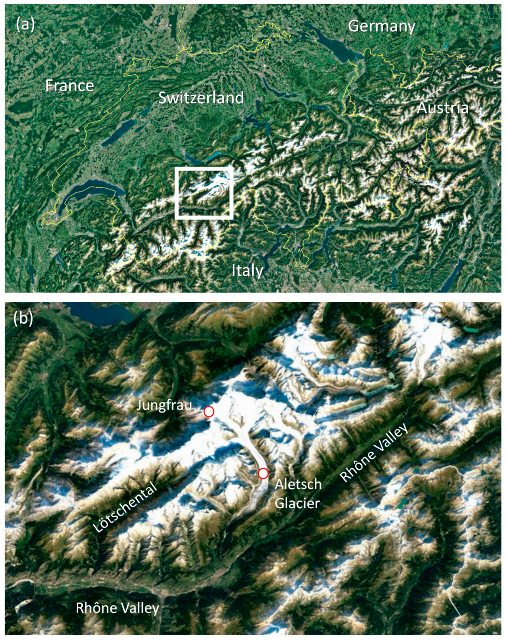
Figure 1. Topographic map of the area under investigation. (a): Switzerland (white rectangle: Lötschental area, modified after [42]). (b): Lötschental area, modified after [43].
Forests 11 00510 g001
Figure 2. Climatic characteristics of Switzerland. (a): Annual precipitation. (b): Annual average temperature. (c): Average relative humidity.
Forests 11 00510 g002
Figure 3. Relative Scheffer Climate Index (SCI), reference location: Uppsala, Sweden, SCI (Uppsala) = 46.3.
Forests 11 00510 g003
Figure 4. Relative annual dose based on different combinations of exposure models (EM 1 and EM 2) and logistic dose–response decay models (LM and SLM). (a): EM1 combined with SLM, (b): EM 2 combined with SLM, and (c): EM 2 combined with LM. Reference location: Uppsala, Sweden.
Forests 11 00510 g004
Figure 5. Relative annual dose in Lötschental based on exposure model EM 2 and the simplified logistic decay model SLM at different resolutions, reference location: Uppsala, Sweden. (a): 7.5 × 7.5 km, (b): 5.0 × 5.0 km, (c): 2.5 × 2.5 km.
Forests 11 00510 g005
Figure 6. Relative annual dose in Lötschental based on exposure model EM 2 and the logistic decay model LM at different resolutions, reference location: Uppsala, Sweden. (a): 7.5 × 7.5 km, (b): 5.0 × 5.0 km, (c): 2.5 × 2.5 km.
Forests 11 00510 g006
Table 1. ParameterAtion [13].
Parameters
a3.2j4.98
e6.75·10−10k−1.8·10−6
f3.50·10−7l9.57·10−5
g7.18·10−5m−1.55·10−3
h7.22·10−3n0.0417
i0.34
Table 2. Degree of determination R2 for linear correlations between the relative doses based on different model combinations and the parameters altitude, precipitation, average relative humidity, and average annual temperature.
Relative Dose [-]
ParameterEM 1/SLMEM 2/LMEM 2/SLMSCI 1
Altitude0.99530.51690.85270.6893
Precipitation0.03130.06640.00050.0121
Avg. RH0.13960.36770.23170.1523
Avg. temperature0.95470.47780.83020.6671
1 Relative Scheffer Climate Index.